Abstract
The Shizhuyuan polymetallic deposit in Hunan Province, China, is a world-class ore field rich in tungsten (W), tin (Sn), molybdenum (Mo), and bismuth (Bi), now facing resource depletion due to prolonged exploitation. This study addresses the limitations of traditional geological prediction methods in complex terrain by integrating multi-source datasets—including γ-ray spectrometry, high-precision magnetometry, induced polarization (IP), and soil radon measurements—across 5049 samples. Unsupervised factor analysis was employed to extract five key ore-indicating factors, explaining 82.78% of data variance. Based on these geological features, predictive models including Support Vector Machine (SVM), Random Forest (RF), and Extreme Gradient Boosting (XGBoost) were constructed and compared. SHAP values were employed to quantify the contribution of each geological feature to the prediction outcomes, thereby transforming the machine learning “black-box models” into an interpretable geological decision-making basis. The results demonstrate that machine learning, particularly when integrated with multi-source data, provides a powerful and interpretable approach for deep mineral prospectivity mapping in concealed terrains.
1. Introduction
With the rapid advancement of data science and artificial intelligence, machine learning (ML) has become an increasingly valuable tool in mineral resource prediction. The pioneering work by Brown et al. introduced artificial neural networks into mineral prospectivity mapping, setting the stage for broader applications of ML in geosciences [1,2]. Since then, algorithms such as Support Vector Machines (SVM) and Random Forests (RF) have demonstrated considerable success in integrating and analyzing geological and geochemical data. Li et al. adopted text mining technology combined with machine learning algorithms to automatically extract ore-prospecting information from a large number of geological studies and constructed an effective deposit prediction model [3]. Carranza et al. demonstrated the potential of ML in geological exploration by combining logistic regression analysis with RF models to evaluate gold mineralization in the Baguio district, Philippines [4]. Zuo et al. emphasized the synergy between geological domain knowledge and computational modeling, highlighting the transformative potential of data-driven exploration strategies [5].
The application of machine learning in mineral resource exploration in Mainland China and abroad is increasing year by year. In Nigeria, exploration work mainly prioritizes direct geological, geochemical, or lithological indicators, often ignoring magnetic signals in the analysis workflow. To bridge this gap, advanced feature extraction based on analytical signals is utilized, and tuned Random Forest (RF) and Gradient Boosting (GB) classifiers are employed to predict the metallogenic structures of complex basement rocks in northern Nigeria [6]. In Xinjiang, China, the Ashile copper–zinc deposit was selected as a case study. Geological and geochemical indicators closely related to mineralization in the study area were extracted, and multiple different labeled datasets were generated from existing boreholes. Support vector machines and random forests were used to address the mineral prospectivity mapping problem in the area surrounding the Ashile copper–zinc deposit [7].
Despite promising progress, significant challenges remain. A key limitation is the scarcity of high-quality, spatially resolved mineralization data, which complicates the training and validation of ML models. Furthermore, the heterogeneity and sparsity of multi-source datasets introduce uncertainty into predictive outcomes, often requiring sophisticated preprocessing and dimensionality reduction techniques to extract meaningful patterns. Addressing these challenges is essential for developing robust, generalizable models for mineral prospectivity mapping [8].
The Shizhuyuan ore district in Hunan Province, China, is a world-renowned polymetallic metallogenic belt enriched in W, Sn, Mo, and Bi. With shallow ore bodies largely exhausted, exploration efforts are now focused on identifying deep-seated and concealed mineralization zones. However, conventional prospecting methods are hindered by thick overburden, dense vegetation, and complex geological structures [9]. In recent years, researchers have increasingly turned to multi-source geophysical and geochemical techniques, such as γ-ray spectrometry, radon surveys, and induced polarization, to improve deep-targeting capabilities. Yet, the predictive value of individual datasets remains limited when used in isolation.
Guo Yueyue et al. carried out soil radon concentration measurements in this area and analyzed the relationship between the fractal distribution of soil concentration and mineralization anomalies [10]. Liu Youjian et al. explored the migration of deep element geo-gas and mineralization anomalies through quantitative geochemical measurements of soil elements [11]. Le O. et al. studied the indicative effect of the geochemical characteristics of plant trace elements in this area on deep mineralization anomalies [12]. Existing studies have shown that various geophysical and geochemical survey data obtained in this area have a weak indicative effect on deep mineralization anomalies.
Consequently, this study proposes a comprehensive ML-based framework for mineral prospectivity mapping that integrates γ-ray spectrometry, magnetometry, radon measurements, and IP data. Unsupervised factor analysis is employed to reduce dimensionality and extract ore-indicating factors, which are then used to train and evaluate SVM, RF and XGBoost models. This study aims to: (1) detect and integrate multi-source data related to mineral prospectivity mapping as mineral exploration indicators; (2) construct predictive models using Support Vector Machine (SVM), Random Forest (RF), and Extreme Gradient Boosting (XGBoost) algorithms, and evaluate model performance with training and testing datasets; (3) conduct SHAP interpretation to reveal key ore-controlling factors, and assess the mineral resource potential of the Jinshiling Area using the optimized machine learning models.
2. Geological Setting
The Shizhuyuan polymetallic metallogenic district is situated within the Nanling Metallogenic Belt in southern China (Figure 1), a region well-known for its abundance of non-ferrous metal deposits including tungsten (W), tin (Sn), molybdenum (Mo), bismuth (Bi), lead (Pb), and zinc (Zn). Several world-class deposits have been identified within this belt, most notably the Shizhuyuan W-Sn-Bi-Mo deposit, which is among the largest of its kind globally [13]. The genesis of these mineral deposits is closely associated with Yanshanian magmatic activity. Central to this mineralization is the Qianlishan granite complex, which exhibits a concentric zoning pattern in plan view, indicative of magmatic-hydrothermal processes [14]. Two primary deposit types are present in the district. Skarn-greisen type W-Sn-Mo-Bi deposits, such as those at Shizhuyuan and Yejwei, are typically located at the contact zones of the Qianlishan granite body [15]. Meanwhile, hydrothermal vein-type Pb-Zn-Ag deposits, including Congshuban, Shexingping, and Hengshanling, occur in carbonate strata at varying distances from the granitic center. The Devonian sedimentary rocks within the district, which have been significantly altered by magmatic intrusions and faulting, serve as key metallogenic host formations [16].
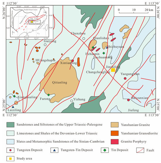
Figure 1.
Geological Overview of the Study Area (Adapted from Reference [17]).
The research area of this study is located in the Jinshiling region, approximately 10 km south of the Shizhuyuan main mining zone (Figure 2). Stratigraphically, the area is composed of rocks from the Devonian, Cambrian, and Sinian periods, overlain by Quaternary sediments. Structurally, the region is characterized by a complex fault system dominated by north–south trending faults, supplemented by northeast (NE), northwest (NW), and east–west (EW) trending faults. These structural features provide favorable pathways for hydrothermal fluid migration, enhancing mineralization potential. Preliminary geological investigations in the area have also reported occurrences of Pb-Zn mineralization, underscoring its potential for further exploration (Figure 3).
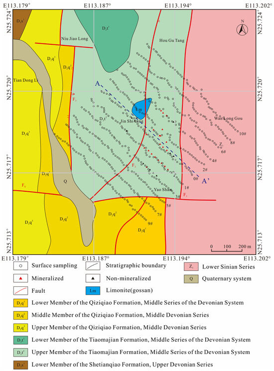
Figure 2.
Layout Diagram of Surface sampling in the Jinshiling Polymetallic Mining Area. #0–#10 represent different wiring configurations.
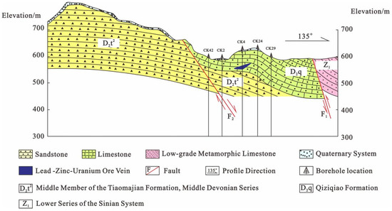
Figure 3.
Geological Cross-Section.
3. Materials and Methods
To construct a comprehensive multi-source geological dataset, a suite of geophysical and geochemical measurements was conducted in the study area. The data acquisition included γ-ray spectrometry, high-precision magnetometry, soil radon concentration measurements, and induced polarization (IP) surveys. Each method was selected for its ability to provide specific indicators related to subsurface mineralization. The γ-ray spectrum can be used to study the possible relationship between mineralization processes and the migration and enrichment of elements such as uranium, thorium, and potassium. By measuring the contents of these elements, it helps to understand the geochemical background of mineralization and provides clues for analyzing the genesis of ore deposits [18]. The γ-ray spectrum was measured using an HD-2002 portable γ-ray spectrometer (Beijing Research Institute of Uranium Geology, Beijing, China) to determine the contents of uranium (U), thorium (Th), potassium (K), and other elements. The system maintained an accuracy threshold within 7% and a relative error sensitivity of ±5%. The average uranium content is approximately 4.90 μg/g, with a standard deviation of 4.67 μg/g, indicating a certain degree of data dispersion. This suggests that the distribution of uranium content may be influenced by a few high-value points, which affect the overall distribution. The average thorium content is about 13.32 μg/g, and its distribution is relatively more concentrated compared to that of uranium. A systematic grid survey method was employed, with a resolution of 10 m between measurement points. In areas exhibiting large fluctuations between adjacent measurements, repeated readings were taken to ensure data reliability until consistent values were achieved. Magnetic measurements were carried out using WCZ-series proton magnetometers (Nanjing Geological Instrument Factory, Nanjing, Jiangsu Province, China), which captured the total magnetic field intensity (in nanoteslas, nT). Instrument calibration and noise assessments were conducted both before and after field measurements to validate data accuracy and consistency. Since the presence of underground ore bodies may alter the migration and distribution of underground gases, and radon is a gas that is relatively sensitive to geological structures and ore bodies, measuring soil radon concentrations can indirectly detect the existence of hidden underground ore bodies or abnormal areas above ore bodies, providing directions for further exploration. Therefore, soil radon concentration measurements are conducted. Soil radon concentrations were measured using the RAD-7 continuous radon detector (Durridge Company, Inc., Bedford, NH, USA), utilizing ion adsorption to determine both instantaneous and average concentrations over fixed time intervals [19]. The “sniffing” mode was employed with a 5-min measurement period, repeated three times per point. To minimize atmospheric interference, a steel probe with a 0.5 cm radius was used to drill holes approximately 70 cm deep. The mean of three cycles was taken as the radon value for each sampling point. Induced polarization (IP) surveys (Zhejiang Huakun Geophysical Instrument Co., Ltd. Hangzhou, Zhejiang Province, China) were conducted using a frequency-domain polarization instrument. A dual-frequency current was injected into the subsurface, and the potential differences at high and low frequencies were measured to assess subsurface electrochemical reactivity. This method provides critical insight into the distribution of concealed ore bodies based on electrical characteristics such as apparent polarizability and resistivity.
All measurements followed standardized survey protocols, employing a grid layout with survey lines oriented northwest-perpendicular to the regional geological formations. A total of 11 survey lines were established, each containing 51 sampling points, resulting in 5049 total measurements. Variables collected included radon concentration, magnetic intensity, uranium, thorium, potassium, total radiation, thorium/uranium ratio, apparent polarizability, and apparent resistivity.
All computational methods used in this study were implemented under Python (Version 3.8. Python Software Foundation, Wilmington, DE, USA). Specifically, data standardization, Principal Component Analysis (PCA), unsupervised factor analysis, Support Vector Machine (SVM), and Random Forest (RF) employed in the study were all conducted by combining different functional methods under the scikit-learn library (Version 1.2) with the collected data for data analysis and integration, and partial machine learning-based mineral prediction results were obtained. The seaborn library (Version 0.12) was used to generate heatmaps. For the construction of the XGBoost model (applied to mineral prospectivity prediction), the xgboost library (Version 1.7.5) was utilized. Additionally, the shap library (Version 0.41) was adopted for model interpretability analysis, which involved calculating SHAP values, plotting feature importance charts, and quantifying the contribution of each feature to mineralization prediction.
4. Multi-Source Data Preprocessing and Traditional Methods Integrated Mineral Prospectivity Mapping
4.1. Data Standardization
Given the heterogeneous nature of the collected datasets, originating from diverse geophysical and geochemical surveys and characterized by varying units, scales, and magnitudes, standardization is a critical preprocessing step. Without normalization, disparities in data dimensions may bias the analysis, particularly in algorithms sensitive to magnitude differences, such as correlation analysis and machine learning models.
where is the original data and is the standardized data. The normalized data conforms to the standard normal distribution with a mean of 0 and a standard deviation of 1.
4.2. Correlation Analysis
In the scope of geological and geophysical data processing, a basic step is to check the correlation between variables to determine the common factors that mark mineralization. The correlation coefficient of the sample data is calculated by the formula:
In order to determine the correlation between the multi-source data, the correlation coefficient between the variables was calculated, and the multi-source data correlation heatmap was constructed (Figure 4).
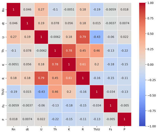
Figure 4.
Correlation heat maps of multi−source data.
- (1)
- There is a very strong positive correlation (about 0.79) between uranium content and total radioactivity content. This strong positive correlation indicates that the total radioactivity content increases with the increasing uranium content. The correlation between U and This not obvious, uranium and thorium are not always enriched at the same time in some places. This might be due to different ore-forming processes or different geochemical environments.
- (2)
- There is also a strong positive correlation (about 0.78) between thorium content and potassium content, implying that they share some kind of common source or behavior in geological processes.
- (3)
- There is a clear negative correlation between uranium content and thorium/uranium ratio (Th/U) (about −0.43). This means that the thorium content may be low even if the uranium content is high in a place, resulting in a lower Th/U ratio.
- (4)
- There is a positive correlation (about 0.61) between potassium content and total radioactivity content. The observed positive correlation between potassium concentration and total radioactivity may primarily arise from the presence of the radioactive isotope 40K, which contributes to beta and gamma emissions. However, this relationship could also be influenced by co-occurring radionuclides (e.g., 226Ra, 228Ra) in mineralized water systems, as both potassium and radium isotopes are often enriched in high-salinity environments.
- (5)
- The low correlation of the magnetic method data (dt) with other variables may indicate that the magnetic anomaly is not perfectly consistent with other geochemical features. This may be due to changes in geological structures, such as faults or folds, which may affect the distribution and geophysical properties of minerals.
- (6)
- The apparent polarizability (Fs) and apparent resistivity (P) are negatively correlated with other variables but the correlation is low, and the correlation between these variables may be related to geological origin and metallogenic mechanism.
4.3. Data Dimensionality Reduction Based on Unsupervised Learning Factor Analysis
4.3.1. Factor Analysis
Factor analysis is an unsupervised learning technique used to reduce the latitude of data and extract key information. Given P observed variables and m potential factors (m < P), each observed variable can be expressed as a linear combination of potential factors. Each observed variable Xi (i = 1, 2, ..., p) can be expressed as:
where represents i observed variables; Fj represents the j th potential factor; λij is the factor load, indicating the degree of contribution or influence of the j th factor on the i th observed variable. For the entire data set, the model can be succinctly expressed using matrix notation as:
Here, X is an p × n matrix representing p observations of n observations; A is a p × m matrix, whose element λij represents the factor load between the j th factor and the i th observed variable; F is an m × n matrix representing the factor scores of m potential factors over n observations.
4.3.2. Extraction of Indicator Common Factors
To effectively extract the key variables indicative of mineralization potential, unsupervised factor analysis was applied to the standardized multi-source dataset. The objective was to reduce the dimensionality of the data while retaining the majority of its informational content. In mineral resource prediction research, a cumulative variance contribution rate of 80% has become a widely accepted standard. Geological data usually contain a large amount of noise and redundant information. When the cumulative variance contribution rate reaches more than 80%, it can effectively capture the main variation characteristics in geological processes while excluding secondary interference factors [20]. The core requirement of this study is to “reduce dimensionality while retaining the total variation of data”, rather than separating independent sources or capturing nonlinear relationships. The data are mainly linearly correlated, which does not meet the “independent source mixing” assumption of ICA, and the sample size is not large enough to require the complex nonlinear modeling of autoencoders. Therefore, Principal Component Analysis (PCA) was first conducted, and the eigenvalues and variance contributions of the components were evaluated. According to the criterion that the cumulative variance contribution should exceed 80% (Table 1), five principal common factors were retained. These factors collectively explained 82.78% of the total variance across the original nine indicators, indicating minimal information loss and strong representativeness.

Table 1.
Interpretation of eigenvalues and total variance for factor analysis.
The factor loadings were subjected to orthogonal rotation using the Kaiser Normal Varimax method to enhance interpretability. After six iterations, the rotation converged, and the geological significance of each factor became more distinct. The rotated factor loading matrix (Table 2) was analyzed to determine the dominant variables associated with each factor, allowing for the interpretation of their geological meaning as follows:
Table 2.
Table of factor loads after rotation.
Common Factor 1 (Radioactive Element Factor): This factor is strongly positively correlated with thorium (Th), potassium (K), and total radioactivity (R), and negatively correlated with radon (Rn). For example, the data information of thorium content, potassium content, and total radioactivity content are mainly integrated, and the variance contribution rate is 28.776%. After rotation, their factor loads are 0.907 and 0.900, respectively, with large loads. The high factor loadings of Th and 40K suggest that this component captures both the enrichment of radiogenic elements in local lithologies and their regional-scale distribution patterns. It reflects regions enriched in radiogenic elements, likely related to U-Th bearing hydrothermal systems or specific lithologies with elevated radiogenic content.
Common Factor 2 (Uranium Enrichment Factor): Highly correlated with uranium (U), radon (Rn), and total radioactivity, and negatively correlated with the Th/U ratio. This factor highlights areas with elevated uranium concentrations, possibly linked to secondary uranium enrichment processes or sedimentary-hosted uranium systems. The data information of uranium content, radon concentration, total content and thorium uranium ratio are mainly integrated, and the variance contribution rate is 22.181%. After rotation, their factor loads are 0.889, 0.471, 0.693 and −0.717, respectively.
Common Factor 3 (Magnetic Feature Factor): Exhibits strong loading on magnetic intensity data (dt), indicating magnetic anomalies likely associated with ferromagnetic minerals or igneous intrusions, both of which may serve as geological guides to mineralization. It mainly integrates the magnetic method data information, and its variance contribution rate is 11.197%. After rotation, its factor load is divided into 0.982, indicating that the factor is related to the magnetic characteristics of the region.
Common Factor 4 (Electrical Conductivity Factor): Dominated by apparent polarizability (Fs), this factor captures the electrical response characteristics of subsurface materials. It mainly synthesizes the data information of polarizability, and its variance contribution rate is 10.906%. After rotation, its factor load is 0.963, indicating reflect sulfide mineralization or conductive lithologies associated with ore bodies.
Common Factor 5 (Resistivity–Radon Response Factor): Characterized by a strong positive correlation with apparent resistivity (P) and a negative correlation with radon concentration. This may indicate the presence of resistive formations or fault/fracture zones influencing radon migration and subsurface permeability.
These five common factors serve as condensed indicators of the original multi-source geological attributes and are subsequently used as inputs in mineral prospectivity modeling. The successful reduction in variables not only streamlines model complexity but also enhances the interpretability and generalizability of the predictive framework.
4.3.3. Factor Score
The common factor score coefficient matrix is shown in Table 3. The expression of 5 common factors can be directly written according to the component score coefficient matrix. Through the expression of common factors, we can calculate the factor scores of these 5 common factors, but the original data after standardization need to be substituted into the expression of common factors. The 5 common factors F1, F2, F3, F4 and F5 can be expressed as the following:
Table 3.
Component score coefficient matrix table.
The five common factor scores reflect the overall level of underground mineral substances from different aspects, and it is difficult to make a comprehensive evaluation by using a single common factor score. Therefore, the comprehensive score F is calculated by considering the proportion of variance contribution rate corresponding to each common factor as the weight:
4.4. Traditional Methods Utilize the Integration of Multi-Source Data for Mineral Prospectivity Mapping
The high anomaly zones in the contour maps of single geological parameters are mostly concentrated in the central and southwestern parts of the study area, with no obvious anomalies in the eastern and northern parts. These zones may be potential mineralization areas, whereas no significant anomalies are observed in the eastern and northern parts of the study area. Figure 5 provides a preliminary identification of potential mineralization areas delineated based on individual single geological parameters. However, a single contour map can only reflect the anomaly of a specific parameter and cannot distinguish the geological causes of the anomaly. For instance, the high uranium anomaly in the central area may result from the enrichment of mineralized hydrothermal fluids, or it may be caused by non-mineralized uranium-bearing rock formations; the low magnetic anomaly (from magnetic surveys) may either be associated with the attenuation of magnetic minerals due to the modification by ore-bearing hydrothermal fluids or represent the natural distribution characteristic of weakly magnetic sedimentary rocks. Additionally, the “potential areas” delineated by contour maps contain a large number of non-mineralized interference zones, making it impossible to accurately locate the actual mineralization range.

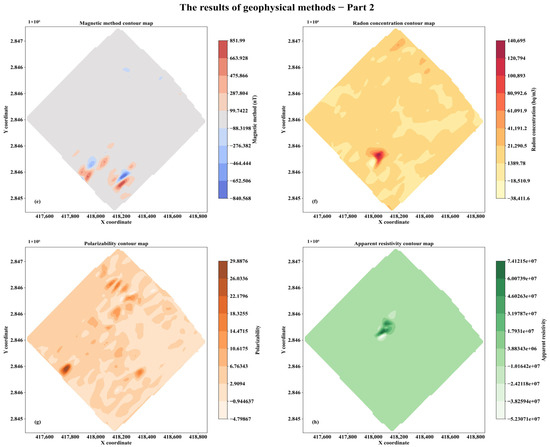
Figure 5.
Contour map of single geological parameter. (a) Uranium content contour map; (b) Thorium content contour map; (c) Potassium content contour map; (d) Total radioactivity contour map; (e) Magnetic method contour map; (f) Radon concentration contour map; (g) Polarizability contour map; (h) Apparent resistivity contour map.
Following the extraction of ore-indicating common factors through factor analysis, traditional geostatistical methods were applied to construct a mineral prospectivity mapping model. The factor scores corresponding to the five principal components were spatially interpolated using the Ordinary Kriging method, which is widely recognized for its accuracy and reliability in geospatial prediction and contour mapping. This approach generated a prospectivity map that visualizes the spatial distribution of potential mineralized zones based on the integrated expression of geophysical and geochemical anomalies.
The resulting mineral prospectivity mapping map (Figure 6) reveals several key insights. High-probability zones, represented by deep red areas, are concentrated primarily in the central and southwestern portions of the study area. These zones are characterized by the convergence of multiple anomaly contours and exhibit strong integrated responses across multiple indicators. Additionally, linear enrichment trends are observed extending southeastward, aligning with known structural features in the region. In contrast, the northwestern and northeastern parts of the study area display weak or negligible mineralization potential.
Figure 6.
Prediction map of potential forming area.
While the integration of multi-source data significantly improves the reliability of geological interpretation compared to single-indicator analyses, limitations remain. Comparison with borehole verification data revealed instances of misclassification and omission, indicating that some high-potential zones were either inaccurately delineated or missed entirely. Moreover, the identified mineralization zones exhibit a fragmented spatial distribution and limited continuity, highlighting the inherent constraints of traditional interpolation-based methods in capturing complex nonlinear relationships within the data.
These findings underscore the need for more advanced analytical approaches that can better accommodate the nonlinear, multi-dimensional nature of geological processes. In response to these limitations, the next phase of this study introduces machine learning models, specifically Support Vector Machines (SVM) and Random Forests (RF), to enhance the accuracy, spatial resolution, and interpretability of mineral prospectivity predictions.
5. Results
5.1. Construction of Training Model
Mineral prospectivity prediction is a multi-phase complex system engineering process. Each phase involves distinct sources of uncertainty that propagate to subsequent stages. The selection of models and uncertainty assessment of results represent another critical challenge in machine learning applications [21].
Support Vector Machine (SVM), a supervised machine learning algorithm, aims to identify an optimal separating hyperplane for a given dataset. This hyperplane must not only effectively classify the samples in the training dataset but also prioritize maximizing its generalization capability to ensure robust performance on unseen data [22].
The support vector machine is as good as possible for generalization ability; that is, the partition hyperplane is as far away from the classification samples in the data set as possible. The generalization ability of the partition hyperplane, as shown in Figure 7, is correspondingly good [23].
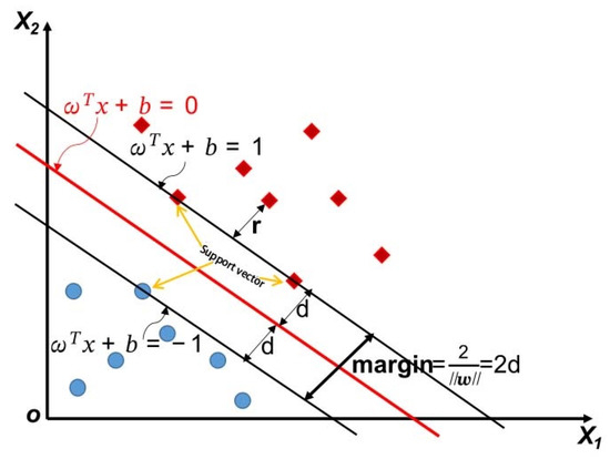
Figure 7.
Support vector, partition hyperplane, and interval.
In the training data sample space, the partition hyperplane can be described by the following linear equation:
Denoting this partition hyperplane as , then the distance from any point X in the training data sample space to the partition hyperplane can be written as:
These data points closest to the partition hyperplane define two decision boundaries, namely and , which are parallel to the optimal hyperplane obtained by the support vector machine. These two decision boundaries are equivalent to defining a region:
There are no more data sample points in the interval defined by the two decision boundaries, the optimal partition hyperplane obtained by the support vector machine is in the middle of this region, and the optimal hyperplane is farthest from the nearest sample of the two categories, which is called the support vector. The sum of the distances between the support vectors of two different classes and the optimal partition hyperplane is:
In order to facilitate the subsequent calculation and narration, it is defined as “margin” in the support vector machine. The essence of support vector machines is to maximize margin, and to maximize the interval, as long as making maximum, it is equivalent to making minimum under the condition of :
In cases where the data is not linearly separable, this study adopts the Gaussian kernel function within the Support Vector Machine (SVM) framework [24]. Although the Gaussian kernel incurs a higher computational cost and longer training times, it is particularly well-suited for scenarios involving high-dimensional feature spaces and limited sample sizes-conditions that are common in fields such as natural language processing and mineral prospectivity analysis. Under such circumstances, the Gaussian kernel offers strong flexibility in capturing nonlinear patterns while maintaining effective generalization.
The Random Forest (RF) algorithm, by contrast, is well known for its robustness and strong generalization capabilities [25]. Its training process involves several key steps. Initially, a technique known as “bagging” (bootstrap aggregating) is used to generate multiple training subsets by randomly sampling the original dataset with replacement. Each subset typically contains about two-thirds of the full dataset. Independent decision trees are then trained on each subset. During the construction of each tree, a random subset of features (less than the total number available) is selected at each node split, thereby promoting model diversity and reducing overfitting. For classification tasks, the final prediction is made by aggregating the outputs of all decision trees using a majority voting mechanism. This ensemble approach enhances both the accuracy and the stability of the model’s predictive performance.
Random forests can use a variety of methods when selecting the optimal attributes of decision tree node splitting, such as information gain and Gini coefficient (), the latter of which is particularly common. The Gini coefficient is calculated as follows:
where fi represents the proportion of Class i samples in the current sample set
5.2. Dataset Partitioning
This study utilized known drill holes to construct a labeled dataset, assigning binary classification labels to each grid cell based on mineralization characteristics (mineralization = 1, non-mineralization = 0) [26]. Mineralized samples (mineralization = 1) are mainly based on mineralization thickness, grade thresholds, and comprehensive geological judgments; non-mineralized samples (non-mineralization = 0) are derived not only from barren boreholes but also from areas with unfavorable geological conditions. The final dataset used for training and evaluation consists of 561 data entries, among which 139 are positive samples (approximately 25%), labeled as the positive class of mineralized structures, i.e., mineralization = 1; and 422 are negative samples (approximately 75%), labeled as the negative class of mineralized structures, i.e., non-mineralization = 0.
This distribution shows obvious imbalance, which has been explicitly addressed during the modeling phase [27]. To ensure the reliability of performance evaluation, methods such as random division, multiple experiments, and spatial cross-validation are adopted to reduce the impact of spatial bias. The dataset is divided into a training set (80%) and a test set (20%). To mitigate the impact of class imbalance during model training, a stratified division method is used for the training and test sets to ensure that the proportion of positive and negative samples in both sets remains consistent. For random forest and extreme gradient boosting models, use the parameter ‘balanced’ to penalize the misclassification of minority classes [28]. For enhanced robustness, this partitioning process was repeated using different random seeds, followed by multiple experimental runs. The final model performance metrics were derived by averaging the results from these repeated runs, thereby mitigating potential biases induced by random data partitioning.
5.3. Mineral Prospectivity Mapping Based on SVM Model and RF Model
To assess the predictive performance of machine learning models in delineating mineralization zones, both the Support Vector Machine (SVM) and Random Forest (RF) algorithms were applied using the five common ore-indicating factors derived from factor analysis as input features [29]. Model optimization was performed via grid search in conjunction with 10-fold cross-validation to identify the most effective hyperparameter configurations, with classification accuracy serving as the evaluation metric.
The optimized SVM model, utilizing a Gaussian kernel function, achieved a maximum classification accuracy of 75% with a penalty parameter C = 1.6 and kernel parameter γ = 0.82. In comparison, the RF model attained an accuracy of 80%, using 15 decision trees and selecting 5 features at each split. These results indicate that the RF model provided superior predictive accuracy for mineral prospectivity mapping. Meanwhile, stopping trigger conditions are set to both retain model efficiency and prevent overfitting, thereby ensuring the robustness of model performance. For the SVM model, the search stops when the decrease in validation accuracy between two consecutive sets of parameters is ≥2%. For the RF model, it stops when the increase in validation accuracy is <1% after the number of decision trees is increased by 20%.
The spatial prediction results for both models are illustrated in Figure 8 and Figure 9. High-probability mineralization zones delineated by both models are primarily concentrated in the central and northeastern parts of the study area, with smaller prospective patches in the eastern and western regions. Validation using known borehole data confirms that the majority of mineralized drill holes fall within the predicted high-probability zones, demonstrating the practical utility of both models. However, the RF model yielded a more focused prediction map, with reduced spatial extent of favorable zones, thereby minimizing false positives in non-mineralized regions.
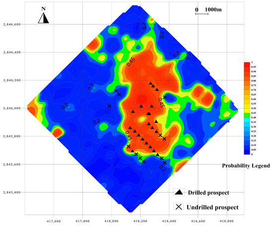
Figure 8.
Probability diagram of mineral prospectivity mapping based on RF.
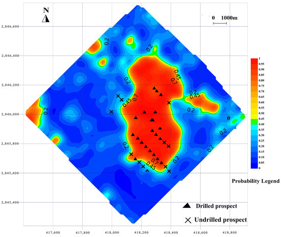
Figure 9.
Probability diagram of mineral prospectivity mapping based on SVM.
In contrast, the SVM model exhibited a tendency to overestimate favorable zones, likely due to its sensitivity to data imbalance. This broader spatial prediction may be beneficial for exploratory targeting but may also lead to increased exploration costs due to reduced precision. Overall, the RF model demonstrated higher accuracy and spatial precision, making it more effective for identifying prospective zones in complex geological settings.
5.4. Mineral Prospectivity Mapping Based on XGBoost Model
XGBoost, as an enhanced Gradient Boosted Decision Trees (GBDT) algorithm, significantly enhances mineral prospectivity mapping model performance by integrating multiple weak learners (decision trees) through iterative optimization. Algorithmically, it employs second-order Taylor expansion to approximate loss functions and introduces regularization terms to control model complexity, thereby improving prediction accuracy and generalization capability. Additionally, its feature quantile approximation and parallel computing optimizations substantially boost computational efficiency, while built-in handling of missing values accommodates common data gaps in mineral datasets. The XGBoost model training was conducted using Python, with the xgboost library version being 1.7.5. In mineral prospectivity mapping, XGBoost demonstrates three core advantages: (1) Efficiency-optimized data structures maximize computational resource utilization, drastically reducing training time; (2) accuracy-weighted voting mechanisms and regularization techniques effectively capture complex geological features and mineralization patterns; (3) flexibility-support for custom loss functions and diverse metrics adapts to varied prediction tasks.
Validation results show an 85% classification accuracy, outperforming RF and SVM. Delineated prospective zones (Figure 10) concentrate in central and northeastern sectors, with drill data confirming: all mineralized holes lie within predicted zones, non-mineralized holes fall outside (indicating minimal false positives/negatives), and most mineralized holes align with high-probability areas-effectively narrowing exploration targets while reducing misclassification of barren areas.
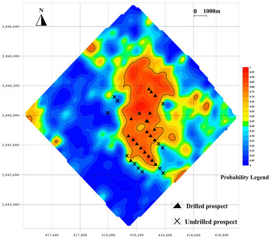
Figure 10.
Probability diagram of mineral prospectivity mapping based on XGBoost.
5.5. Shapley Additive Explanations
To analyze the prediction mechanism of the stacking model, this study employs the SHAP (Shapley Additive exPlanations) interpretable framework to assess the global feature importance. The feature importance is determined by calculating the mean absolute value of the SHAP values (Mean |SHAP|) for each feature, and a feature importance ranking chart (SHAP feature importance ranking chart) is generated based on this ordering [30]. This paper uses Python for SHAP model interpretation, with the SHAP version being 0.41. The results (Figure 11) indicate that the values of P, dt, Th and Rn are significantly higher than those of other variables, suggesting that these features play a dominant role in the prediction of lead–zinc mineralization. The higher its value, the greater the possibility of discovering mineral deposits. Among them, fault zones, fracture systems, and other geological structures usually cause abnormal changes in apparent resistivity (P). These structures may serve as channels for ore fluid migration or sites for mineral precipitation, so apparent resistivity anomalies can indirectly indicate potential mineralized areas [31]. At the same time, magnetic data (dt) can also help identify fault zones, folds, and other geological structures. Therefore, magnetic anomalies can indirectly indicate potential mineralized areas [32]. Thorium (Th), uranium (U), and radon (Rn) are three important radioactive elements. The distribution of thorium can reflect the genesis and evolutionary history of geological bodies, so anomalies in thorium content can indirectly indicate potential mineralization environments [33]. Uranium is the main component of uranium ores, so anomalies in uranium content are a direct indicator for prospecting uranium ores [34]. Radon is a gas that can migrate from deep mineralized areas to the surface, so radon anomalies can indicate deep uranium mineralization [35].
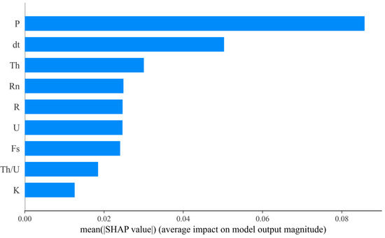
Figure 11.
SHAP feature importance ranking chart.
Although the feature importance chart can provide a global ranking of feature weights for model predictions, its scalar output makes it difficult to characterize the distribution of contributions of individual features to the prediction results. This study generates a SHAP summary plot for each feature, where each sample point in the plot represents the SHAP value corresponding to a specific feature. The distribution position of data points on the horizontal axis indicates the direction and intensity of the feature’s influence: a shift in the positive direction (to the right) reflects an enhancement of the positive promoting effect, while a shift in the negative direction (to the left) indicates an increase in the negative inhibitory effect. The y-axis lists all model features, sorted by their overall importance, with the most influential features located at the top. Feature values are presented through color gradient mapping, and the color bar on the right shows a continuous change from blue (low feature values) to red (high feature values). As shown in Figure 12, features such as P (apparent resistivity), Th (thorium), and U (uranium) exhibit a significant positive correlation with the mineralization of lead–zinc deposits. When these feature values increase, their SHAP values increase simultaneously, indicating a significant improvement in the probability of mineralization in the corresponding areas. It is worth noting that the surrounding rock contact zone buffer feature shows a strong negative correlation, which has an obvious inhibitory effect on the formation of ore deposits. The P parameter shows a significant indicative effect on sulfide ore bodies, which is highly consistent with the electrical characteristics of known lead–zinc mining areas. The dt magnetic data shows a negative correlation: areas with low dt magnetic values are more likely to correspond to the aforementioned weakly magnetic ore-hosting rocks or altered zones, thus better indicating the potential presence of lead–zinc–uranium ores in the region.
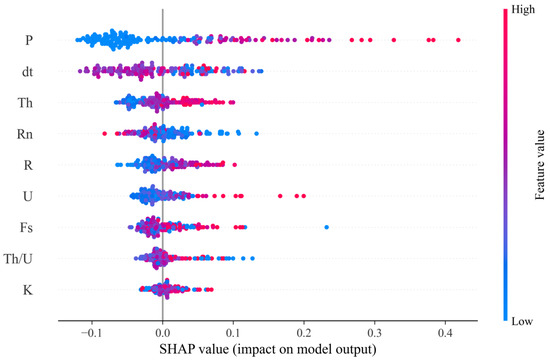
Figure 12.
SHAP summary plot for each feature.
As Th, U, Fs, Th/U, and K increase, their SHAP values also increase, indicating that areas with higher element concentrations are more likely to form ore deposits. The first step in using SHAP data to guide exploration decisions is to identify which features are most important for mineralization prediction. This can be achieved by analyzing the SHAP feature importance ranking chart (Figure 11). Determining the thresholds of these features based on SHAP values, as quantitative criteria for exploration decisions, helps convert complex model predictions into actionable exploration guidelines [36]. Mineralization prediction is usually based on a comprehensive analysis of multiple geological and geophysical features. Using SHAP data, the contribution of different feature combinations to mineralization prediction can be quantified, guiding multi-feature combination decisions, thereby dividing exploration target areas at different levels [37]. Priority should be given to exploring areas with high potential and low uncertainty [38]. For example, if the value of apparent resistivity is high, priority should be given to electrical prospecting; if the values of thorium, uranium, and radon are high, radioactive measurement should be strengthened.
6. Discussion
This study evaluated the performance of three mineral prospectivity mapping models-Random Forest (RF), Support Vector Machine (SVM), and XGBoost-using Receiver Operating Characteristic (ROC) curve analysis (Figure 13). Among the models, the XGBoost achieved the highest Area Under the Curve (AUC) value of 0.863, indicating excellent classification capability. The standard RF model followed with an AUC of 0.841 while the SVM model showed the lowest performance with an AUC of 0.651.
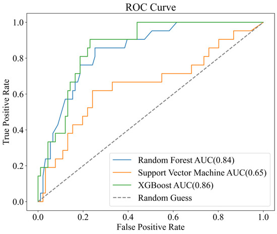
Figure 13.
ROC curves of mineralization probability prediction graphs based on different models.
Further validation using confusion matrix-derived metrics reinforced these findings (Table 4). The XGBoost model not only delivered the highest accuracy (85%) but also achieved a recall of 0.728, effectively narrowing the spatial extent of predicted mineralized zones and minimizing false negatives. In comparison, the RF model yielded a recall of 0.791, while the SVM model, despite delineating the broadest favorable areas, recorded the lowest recall at 0.602. This inverse relationship between recall and target zone breadth highlights the trade-off between model sensitivity and spatial precision in mineral prospectivity analysis.
Table 4.
Machine learning model evaluation parameters.
Overall, the XGBoost model demonstrated superior performance across all evaluation metrics, establishing itself as the most effective and reliable approach for deep mineral exploration in complex geological settings.
Due to the inherent black-box nature of machine learning models, their prediction processes are difficult to interpret, as introduced in the literature. There is a need for a framework for data-driven mineral prospectivity mapping with interpretable machine learning and modulated predictive modeling. This has become a bottleneck hindering the widespread application of machine learning-based mineral prospectivity mapping models in the industry [39].
To improve model transparency, this study employs a globally interpretable algorithm (SHAP) for analysis. Combined with the newly obtained distribution data of radioactive elements such as Th and U through γ-ray spectrometry, as well as the magnetic anomaly data measured by high-precision magnetometers. The results show that variables P, Th, R, U, Fs, Th/U, and K have a significant positive impact on the formation of lead–zinc–uranium deposits, meaning that an increase in their values is associated with an enhancement in mineralization potential. In contrast, dt exhibits a strong negative impact: a decrease in magnetic anomaly intensity is positively correlated with the probability of mineralization. The infiltration of ore-forming fluids causes the alteration of magnetic minerals in the surrounding rock into weakly magnetic minerals, leading to the attenuation of magnetic anomalies [40]. Negative magnetic anomalies often coincide with fracture zones and structurally fractured areas, which are favorable channels for hydrothermal migration and mineral precipitation, suggesting a higher probability of discovering lead–zinc deposits.
The Jinshiling mining area is located between two large faults, with a large depression zone in the middle. Such geological conditions are conducive to the migration and accumulation of minerals. The main strata include the Sinian (Z1) epimetamorphic sandstone, tuffaceous arkose, and slate; the Middle Devonian Tiaomajian Formation (D2t) sandstone, dolomitic limestone, and Qiziqiao Formation (D2q) limestone; and the Upper Devonian Shetianqiao Formation (D3s) argillaceous limestone and clastic rocks, while the ore deposit strata are dominated by limestone. Due to the significant differences in physical properties at these lithological interfaces, fracture zones and fissures are prone to form under tectonic stress, providing favorable conditions for the migration of ore-bearing fluids and the precipitation of minerals [41]. Meanwhile, at the contact interfaces of different lithologies, due to differences in chemical properties, metasomatism and replacement reactions are likely to occur, promoting the precipitation and enrichment of minerals. Fault structures are not only important ore-controlling factors but also significant sources of geophysical anomalies. Near fault zones, magnetic data anomalies may occur due to pyritization and pyrrhotitization; electrical anomalies with low resistivity and high polarizability may appear due to sulfide mineralization. These geophysical anomaly characteristics can serve as important markers for identifying fault structures. The oxidation degree of mineral elements in the Jinshiling area is relatively high, with the oxidation rates of zinc and lead being 27.4% and 36%, respectively, indicating that the chemical conditions for mineralization are very favorable. The ores mainly include lead–zinc pyrite and lead–zinc ore. Since the ore bodies are mainly composed of lead–zinc sulfides, which have good electrical conductivity and form obvious electrical differences with the surrounding country rocks, corresponding electrical anomalies can be detected through electrical prospecting. Along the southward strike, the concentrations of sulfur and lead generally decrease, but the grade increases with depth. Combined with data obtained by geophysical methods such as γ-ray spectrometry, it further indicates the spatial variation in mineral concentrations and the influence of geological structures on mineral distribution.
Traditional methods have difficulty quantifying the spatial correlation between fault structures and mineralization in the Jinshiling area. In this study, through SHAP value analysis, combined with apparent resistivity data and data obtained by γ-ray spectrometry, it is found that the mineralization probability increases in the coupling area of low magnetic anomalies and high apparent resistivity in this area. Compared with traditional statistical methods (such as weight of evidence, logistic regression), which have limited ability to characterize nonlinear geological relationships and are susceptible to artificial experience bias, this study reveals the nonlinear mechanism of action of key features through the SHAP interpretable framework, solving the decision-making uncertainty caused by the “black box model” in traditional methods [39].
Lead–zinc ore bodies (especially sulfide-rich zones) often exhibit high resistivity anomalies due to their high content of conductive minerals (such as galena and sphalerite). The Th/U ratio indicates oxidized alteration zones where uranium has migrated and been lost, which is often related to the activity of ore-forming fluids. This finding is consistent with the conclusions of previous studies [42]. By combining the distribution of deposit locations identified by machine learning with a small number of drilling projects (the ores in this area are mainly divided into two types: lead–zinc pyrite and lead–zinc ore), and referring to the areas with abnormal radon concentration in soil radon concentration measurements, it is found that there are concealed Pb-Zn-U polymetallic ore bodies in this area, making it a potential mineralization prospect area. These findings are basically consistent with the conclusions of previous studies.
Mineralization in the Jinshiling area is controlled by north–south trending faults and their secondary northeast/northwest/east–west trending faults. The ore deposits are associated with the contact zones of the Qianlishan granite and Devonian carbonate strata. Machine learning models (XGBoost, Random Forest, Support Vector Machine) show strong spatial consistency with these geological settings, with their high-potential areas concentrated at fault intersections, granite–carbonate contact zones, and depression zones between large faults—all of which are favorable for the accumulation of hydrothermal minerals. Regarding geophysical maps, γ-ray spectrometry anomalies (uranium > 6 μg/g, thorium > 18 μg/g) overlap with the machine learning-predicted areas, and SHAP analysis confirms that uranium and thorium are key predictors; low values of high-precision magnetometry are consistent with the model results, as low magnetic intensity (dt) is negatively correlated with the probability of mineralization; soil radon anomalies (>5000 Bq/m3, related to faults) are consistent with high-potential areas, and radon (Rn) has a significant weight in XGBoost; induced polarization anomalies (high polarizability Fs, specific resistivity P range) match the predicted lead–zinc mineralization areas; and the derived parameters of induced polarization (P, Fs) have a significant impact on the model results. It is worth noting that XGBoost (with an accuracy of 85%) outperforms traditional methods by capturing the nonlinear relationships between multi-source signals and geological structures, overcoming the limitation of scattered anomalies in single geophysical maps, thus providing a more reliable mineralization potential prediction map.
7. Conclusions
The accuracy of traditional methods, such as geological mapping combined with single-element anomaly delineation, in predicting concealed lead–zinc–uranium deposits in the Jinshiling area is less than 60%, and the overlap rate between target areas and known mineralized zones is low. Their prediction results have problems of scattered spatial distribution and poor continuity, and compared with borehole verification data, there are also phenomena of misjudgment and omission. However, in this area, machine learning methods have shown significant advantages. Traditional methods need to arrange 120 verification boreholes to delineate high-potential areas, while machine learning methods completed the positioning of mineralized zones with only 33 verification holes, compressing the range to 28% of the original range, which greatly saved exploration costs. This fully highlights the limitations of traditional methods in capturing complex nonlinear relationships in data, while machine learning models have effectively overcome this problem.
In the data collection and processing stage, this study collected a total of 5049 multi-dimensional data by integrating various data such as γ-ray spectrometry, high-precision magnetic measurement, and soil radon concentration, and conducted standardized analysis on them to ensure the consistency and reliability of the data. The average radon concentration is 4865.74 bq/m3, with a standard deviation of 8020.84 bq/m3, indicating a large degree of data dispersion. The high-value areas may imply the existence of underground radioactive element enrichment zones, fault zones, or areas with active geological tectonic activities. The magnetic measurement values range from −1277.00 nT to 825.00 nT. Changes in magnetic anomalies reflect differences in the magnetic properties of underground rocks. Negative values may be related to weakly magnetic rocks or underground magnetic interference, while positive values may correspond to strongly magnetic rocks. The average polarizability is 3.42, and areas with high polarizability may be related to metal sulfide mineralization and the like. The standard deviation of apparent resistivity is extremely large, and significant changes reflect the differences in the electrical properties of underground media. Low apparent resistivity may be related to water-bearing strata and metal mineralization, while high apparent resistivity may correspond to dry rocks or bedrock [43].
Subsequently, factor analysis was used to extract 5 common ore-indicating factors from these data, which effectively retained key geological information while significantly reducing the data dimension, laying a foundation for the efficient operation of subsequent machine learning models. In the model construction and evaluation stage, two widely used machine learning models, SVM and RF, were developed and evaluated with the extracted factors as inputs. It was found through comparison that the RF model is superior to the SVM model in both accuracy and spatial precision. To further improve the model performance, the XGBoost algorithm was introduced, which achieved a classification accuracy of 85% and an AUC value of 0.863. In addition, the SHAP interpretable model was introduced to analyze and summarize specific elements to explain the “black box” nature of machine learning models, providing a new research direction for mineral exploration. The prediction results generated by the XGBoost model are more geologically reasonable, all known mineralized boreholes are correctly classified, and the false positive rate is minimized. This indirectly proves the reliability of our prediction model, and the high mineralization potential areas that have not been drilled can be used as potential targets for future mineral surveys.
Author Contributions
J.X.: Writing—original draft, Visualization, Software, Validation, Methodology, Investigation, Data curation, Conceptualization. Y.L.: Writing—review & editing, Validation, Supervision, Project administration. W.L.: Writing—original draft, Data curation, Investigation, Methodology, Validation. S.H.: Validation, Supervision, Project administration, Methodology, Data curation. K.T.: Writing—review and editing, Validation, Supervision, Project administration, Methodology. Y.X.: Methodology, Investigation, Conceptualization. Y.Z.: Software, Investigation, Conceptualization. All authors have read and agreed to the published version of the manuscript.
Funding
The APC of this article is funded by University of South China. This research received no external funding.
Data Availability Statement
The source codes are available on GitHub at https://github.com/Jie-Xcc/Mineral-Prospecting-Prediction/tree/main (accessed on 29 September 2025).
Acknowledgments
The first author hereby formally acknowledges the co-authors for their critical intellectual engagement and methodological expertise, which significantly contributed to the theoretical and technical refinement of this investigation. Gratitude is extended to the administrative and technical teams of the Shizhuyuan polymetallic mining district, Hunan Province, China, for their operational facilitation of data acquisition protocols.
Conflicts of Interest
The authors declare that they have no known competing financial interests or personal relationships that could have appeared to influence the work reported in this paper.
References
- Brown, M.W.; Gedeon, D.T.; Groves, I.D.; Barnes, R.G. Artificial neural networks: A new method for mineral prospectivity mapping. Aust. J. Earth Sci. 2000, 47, 757–770. [Google Scholar] [CrossRef]
- Yang, F.F.; Wang, Z.Y.; Zuo, R.G.; Sun, S.; Zhou, B. Quantification of Uncertainty Associated with Evidence Layers in Mineral Prospectivity Mapping Using Direct Sampling and Convolutional Neural Network. Nat. Resour. Res. 2023, 32, 79–98. [Google Scholar] [CrossRef]
- Li, S.; Chen, J.; Xiang, J. Prospecting information extraction by text mining based on convolutional neural networks: A case study of the Lala Copper Deposit, China. IEEE Access 2018, 6, 52286–52297. [Google Scholar] [CrossRef]
- Carranza, M.J.E.; Laborte, G.A. Data-driven predictive mapping of gold prospectivity, Baguio district, Philippines: Application of Random Forests algorithm. Ore Geol. Rev. 2015, 71, 777–787. [Google Scholar] [CrossRef]
- Zuo, R. Geodata Science-Based Mineral Prospectivity Mapping: A Review. Nat. Resour. Res. 2020, 29, 3415–3424. [Google Scholar] [CrossRef]
- Abraham, E.; Usman, A.; Amano, I. Machine Learning-Based Classification of Geological Structures from Magnetic Anomaly Data: Case Study of Northern Nigeria Basement Complex. Mach. Learn. Appl. 2025, 20, 100678. [Google Scholar] [CrossRef]
- Zheng, C.; Yuan, F.; Luo, X.; Li, X.; Liu, P.; Meilan, W.; Chen, Z.; Albanese, S. Mineral Prospectivity Mapping Based on Support Vector Machine and Random Forest Algorithm—A Case Study from Ashele Copper-Zinc Deposit, Xinjiang, NW China. Ore Geol. Rev. 2023, 159, 105567. [Google Scholar] [CrossRef]
- DumakorDupey, N.K.; Sampurna, A. Machine Learning—A Review of Applications in Mineral Resource Estimation. Energies 2021, 14, 4079–4407. [Google Scholar] [CrossRef]
- Wu, W.B.; Tan, K.X.; Han, S.L.; Xie, Y.S.; Tan, W.Y.; Guo, Y.Y.; Cai, Q.E. Fractal Analysis of Ground γ-ray Spectrometry Data in Jinshiling Area, Chenzhou, Hunan. J. Univ. South China (Nat. Sci. Ed.) 2018, 32, 20–24. [Google Scholar]
- Guo, Y.Y.; Tan, K.X.; Tan, W.Y.; Han, S.L.; Xie, Y.S.; Wu, W.B.; Cai, Q.E. A Fractal Theory-Based Method for Analyzing Mineralization Anomalies of Soil Radon Concentration: A Case Study of Jinshiling Area, Chenzhou, Hunan. J. Univ. South China (Nat. Sci. Ed.) 2018, 32, 15–19. [Google Scholar]
- Liu, Y.; Xie, Y.; Tan, K.; Han, L.; Wang, P.; Kang, H. Quantitative Geochemical Evidence for Geo-gas Migration of Deep Elements: A Case Study of the Jinshiling Uranium Polymetallic Deposit in Chenzhou. Met. Mine 2020, 146–154. [Google Scholar]
- Le, O.; Tan, K.; Li, Y.; Liu, Z.; Zhou, H.; Li, C.; Xie, Y.; Han, S. Trace Element Geochemical Characteristics of Plants and Their Role in Indicating Concealed Ore Bodies Outside the Shizhuyuan W-Sn Polymetallic Deposit, Southern Hunan Province, China. Minerals 2024, 14, 967. [Google Scholar]
- Zhao, P.L.; Yuan, S.D.; Mao, J.W.; Yuan, Y.B.; Zhao, H.J.; Zhang, D.L.; Shuang, Y. Constraints on the timing and genetic link of the large-scale accumulation of proximal W-Sn-Mo-Bi and distal Pb-Zn-Ag mineralization of the world-class Dongpo orefield, Nanling Range, South China. Ore Geol. Rev. 2018, 95, 1140–1160. [Google Scholar] [CrossRef]
- Mao, J.W.; Li, H.Y. Evolution of the Qianlishan Granite Stock and its Relation to the Shizhuyuan Polymetallic Tungsten Deposit. Int. Geol. Rev. 1995, 37, 63–80. [Google Scholar] [CrossRef]
- Tao, S.; Ma, X. Research progress and major scientific issues of the super-large W-Sn-Mo-Bi deposit in Shizhuyuan, Hunan. Acta Mineral. Sin. 2022, 42, 793–806. [Google Scholar] [CrossRef]
- Cheng, Y.S. Petrogenesis of skarn in Shizhuyuan W-polymetallic deposit, southern Hunan, China: Constraints from petrology, mineralogy and geochemistry. Trans. Nonferrous Met. Soc. China 2016, 26, 1676–1687. [Google Scholar] [CrossRef]
- Peng, J.; Zhou, M.-F.; Hu, R.; Shen, N.; Yuan, S.; Bi, X.; Du, A.; Qu, W. Precise Molybdenite Re–Os and Mica Ar–Ar Dating of the Mesozoic Yaogangxian Tungsten Deposit, Central Nanling District, South China. Miner. Depos. 2006, 41, 661–669. [Google Scholar] [CrossRef]
- Imaizumi, M. Overview on Spectral Analysis Techniques for Gamma Ray Spectrometry. Nucl. Sci. 2024, 9, 8–29. [Google Scholar] [CrossRef]
- Tan, W. Study on the Natural Radiation Environment in the Shizhuyuan Tungsten Polymetallic Mining Area, Chenzhou, Hunan. Ph.D. Thesis, University of South China, Hengyang, China, 2019. [Google Scholar] [CrossRef]
- Olasehinde, A.; Ashano, E. Data Driven Predictive Modelling of Mineral Prospectivity Using Principal Component Analysis: A Case Study of Riruwai Complex. Adv. Appl. Sci. Res. 2021, 12, 33. [Google Scholar]
- Zhang, Z.; Cheng, Q.; Yang, J.; Wu, G.; Ge, Y. Machine Learning and Mineralization Prediction: A Case Study of Iron Polymetallic Ore Prediction in Southwestern Fujian. Earth Sci. Front. 2021, 28, 221–235. [Google Scholar] [CrossRef]
- Qiu, J.; Shi, H.; Hu, Y.; Yu, Z. Enhancing Anomaly Detection Models for Industrial Applications through SVM-Based False Positive Classification. Appl. Sci. 2023, 13, 12655. [Google Scholar] [CrossRef]
- Chetana, K.; Aditya, A. Feature level fusion framework for multimodal biometric system based on CCA with SVM classifier and cosine similarity measure. Aust. J. Electr. Electron. Eng. 2023, 20, 205–218. [Google Scholar]
- Kapil, K. Comprehensive Composition to Spot Intrusions by Optimized Gaussian Kernel SVM. Int. J. Knowl. Based Organ. (IJKBO) 2022, 12, 27. [Google Scholar]
- Chen, J.; Mao, C.; Liu, K.; Deng, H. 3D Mineralization Prediction of Dayingezhuang Gold Deposit Based on Random Forest Algorithm. Geotecton. Et Metallog. 2020, 44, 231–241. [Google Scholar] [CrossRef]
- Xiang, J.; Xiao, K.; Carranza, E.J.M.; Chen, J.; Li, S. 3D Mineral Prospectivity Mapping with Random Forests: A Case Study of Tongling, Anhui, China. Nat. Resour. Res. 2020, 29, 395–414. [Google Scholar] [CrossRef]
- Xiong, Y.; Zuo, R. A Positive and Unlabeled Learning Algorithm for Mineral Prospectivity Mapping. Comput. Geosci. 2021, 147, 104667. [Google Scholar] [CrossRef]
- Senanayake, I.P.; Kiem, A.S.; Hancock, G.R.; Metelka, V.; Folkes, C.B.; Blevin, P.L.; Budd, A.R. A Spatial Data-Driven Approach for Mineral Prospectivity Mapping. Remote Sens. 2023, 15, 4074. [Google Scholar] [CrossRef]
- Wainer, J.; Fonseca, P. How to tune the RBF SVM hyperparameters? An empirical evaluation of 18 search algorithms. Artif. Intell. Rev. 2021, 54, 1–27. [Google Scholar] [CrossRef]
- Lundberg, S.M.; Erion, G.; Chen, H.; DeGrave, A.; Prutkin, J.M.; Nair, B.; Katz, R.; Himmelfarb, J.; Bansal, N.; Lee, S.-I. From Local Explanations to Global Understanding with Explainable AI for Trees. Nat. Mach. Intell. 2020, 2, 56–67. [Google Scholar] [CrossRef]
- Zhang, C.; Yuan, B.; Li, Y.; Zhang, Q.; Han, L. Features of Apparent Resistivity Anomaly of Controlled-Source Audio-Frequency Magnetotellurics and Prospects of Oil Shale in the Tongchuan Area of the Southern Ordos Basin, China. Interpretation 2021, 9, T1055–T1063. [Google Scholar] [CrossRef]
- Lawal, T.O.; Omar, D.M.; Salami, M.K.; Adewumi, T.; Sunday, J.A.; Fawale, O. Detection of Concealed Mineral Deposits Using Magnetic Data in Part of Osun State and Its Environs, South-Western Nigeria. In Proceedings of the IOP Conference Series: Earth and Environmental Science, Ota, Nigeria, 3–5 August 2021; Volume 655, p. 012074. [Google Scholar] [CrossRef]
- Dentith, M.C.; Mudge, S.T. Geophysics for the Mineral Exploration Geoscientist; Cambridge University Press: Cambridge, UK, 2014. [Google Scholar] [CrossRef]
- Jiang, Z.; Han, X.; Lin, Z.; Hu, H.; Lai, Q.; Gu, Y.; Wu, Z.; Zhao, X. Large-Scale Aerial Gamma Spectroscopy for Exploring Sandstone-Type Uranium Deposits: A Case Study of Gexi Area, Inner Mongolia. Appl. Geophys. 2023, 22, 383–672. [Google Scholar] [CrossRef]
- Dyck, W. Development of Uranium Exploration Methods Using Radon. In Geological Survey of Canada; Natural Resource Canada: Ottawa, ON, Canada, 1969; pp. 46–69. [Google Scholar]
- Kang, K.; Chen, Q.; Wang, K.; Zhang, Y.; Zhang, D.; Zheng, G.; Xing, J.; Long, T.; Ren, X.; Shang, C.; et al. Application of Interpretable Machine Learning for Production Feasibility Prediction of Gold Mine Project. Appl. Sci. 2023, 13, 8992. [Google Scholar] [CrossRef]
- Yousefi, M.; Kreuzer, O.P.; Nykänen, V.; Hronsky, J.M.A. Exploration Information Systems—A Proposal for the Future Use of GIS in Mineral Exploration Targeting. Ore Geol. Rev. 2019, 111, 103005. [Google Scholar] [CrossRef]
- Davies, R.S.; Davies, M.J.; Groves, D.; Davids, K.; Brymer, E.; Trench, A.; Sykes, J.P.; Dentith, M. Learning and Expertise in Mineral Exploration Decision-Making: An Ecological Dynamics Perspective. Int. J. Environ. Res. Public Health 2021, 18, 9752. [Google Scholar] [CrossRef] [PubMed]
- Mou, N.; Carranza, E.J.M.; Wang, G.; Sun, X. A Framework for Data-Driven Mineral Prospectivity Mapping with Interpretable Machine Learning and Modulated Predictive Modeling. Nat. Resour. Res. 2023, 32, 2439–2462. [Google Scholar] [CrossRef]
- Deng, J.; Wang, Q.; Gao, L.; He, W.; Yang, Z.; Zhang, S.; Chang, L.; Li, G.; Sun, X.; Zhou, D. Differential Crustal Rotation and Its Control on Giant Ore Clusters along the Eastern Margin of Tibet. Geology 2020, 49, 428–432. [Google Scholar] [CrossRef]
- Zhao, D.; Han, R.; Liu, F.; Fu, Y.; Zhang, X.; Qiu, W.; Tao, Q. Constructing the Deep-Spreading Pattern of Tectono-Geochemical Anomalies and Its Implications on the Huangshaping W–Sn–Pb–Zn Polymetallic Deposit in Southern Hunan, China. Ore Geol. Rev. 2022, 148, 105040. [Google Scholar] [CrossRef]
- Constable, S. Ten Years of Marine CSEM for Hydrocarbon Exploration. Geophysics 2010, 75, A67–A81. [Google Scholar] [CrossRef]
- Tsae, N.B.; Adachi, T.; Kawamura, Y. Application of Artificial Neural Network for the Prediction of Copper Ore Grade. Minerals 2023, 13, 658. [Google Scholar] [CrossRef]
Disclaimer/Publisher’s Note: The statements, opinions and data contained in all publications are solely those of the individual author(s) and contributor(s) and not of MDPI and/or the editor(s). MDPI and/or the editor(s) disclaim responsibility for any injury to people or property resulting from any ideas, methods, instructions or products referred to in the content. |
© 2025 by the authors. Licensee MDPI, Basel, Switzerland. This article is an open access article distributed under the terms and conditions of the Creative Commons Attribution (CC BY) license (https://creativecommons.org/licenses/by/4.0/).