A Novel Method of Magnetic Sources Edge Detection Based on Gradient Tensor

Abstract

The edge detection method based on the magnetic gradient tensor data plays an important role in magnetic exploration because it is free from geomagnetic interference and contains more abundant information. This paper proposes a new anomaly edge detection method using the magnetic gradient tensor components. The model is established to compare with other methods, such as directional total horizontal derivative (THD_z), analytical signal (AS), tilt angle, theta map, and so on, under conditions of vertical magnetization, oblique magnetization, and noise interference. Through the study of the anomaly distribution of the rectangular model, it is observed that the edge detection method proposed in this paper is nearly impervious to noise interference, exhibits strong anti-interference capabilities, delivers a high-quality boundary identification effect, and provides greater accuracy in anomaly edges with minimal error. When multiple anomalous bodies are present, the edge detection results are less susceptible to interference from each other, resulting in higher resolution. The efficiency of the algorithm is demonstrated by real magnetic data from some study areas in Jiangxi Province, China. The experimental results show that the proposed method is more precise and accurate than the total horizontal derivative, analytical signal, tilt angle, and theta map methods.

1. Introduction

The magnetic exploration method is one of the important geophysical exploration methods that directly reveals the anomaly information related to ferromagnetic minerals, attracting widespread attention [1,2]. In previous studies, most of the methods for locating magnetic anomalies were realized by using the total magnetic intensity as well as the magnetic vector [3]. However, the information on subsurface anomalies obtained through the total magnetic field strength and magnetic field vector methods is limited. With the progress and development of science and technology, magnetic exploration has evolved from total magnetic field measurement to magnetic gradient tensor measurement [4] and magnetic scalar measurement to magnetic vector measurement [5]. Furthermore, significant advancements have been made in data processing methods for magnetic exploration.

In the previous studies of magnetic gradient tensor data, it was common practice to convert total field data for processing [6]. Currently, magnetic gradient tensor data can be directly measured using the superconducting quantum interference device (SQUID) [7,8,9,10]. The measured magnetic gradient tensor data has many advantages [11,12,13], such as it will not be interfered with by the geomagnetic field [14], it will be less affected by the distribution pattern of the underground anomalies, the spatial resolution is higher, the magnetic anomaly information is more abundant [15], and it has better real-time characteristics, etc. [16]. Therefore, the magnetic gradient tensor data have attracted widespread attention. Utilizing magnetic gradient tensor data for anomaly localization and boundary identification has also become a hot spot in current research.

Many scholars have studied the method for edge identification of magnetic gradient tensor data. Nabighian [17] proposed using the analytic signal method to process two-dimensional anomalous data. Roest et al. [18], Qin [19], and Nabighian [20] extended the analytic signal method to 3D anomaly data. Beiki [21] defined the directional analytic signal and combined the analytic signal with the Hilbert transform to enhance the boundary identification effect, but this method is sensitive to noise. Yuan and Yu [22,23] defined a new boundary identification method of the gradient tensor data by using the horizontal directional analytical signal and the second-order derivative of the horizontal directional analytical signal. The maximum value calculated by the improved method is usually regarded as the field source boundary. Miller and Singh [24] proposed the identification of anomaly boundaries by using the tilt angle, which is the arctangent of the ratio of the vertical and horizontal components. This method can assess the quantity and distribution of anomalies at different depths but is significantly affected by the direction of the magnetization [25]. Gang et al. [26] improved the tilt angle to estimate the horizontal position of multiple dipole-like magnetic field sources. Ferreira et al. [27] used tilt angle to enhance the total horizontal derivative of magnetic anomalies to identify the boundary of abnormal bodies. Verduzco et al. [28] computed the tilt angle of the total horizontal derivative to recognize the edges. Wijns et al. [29] measured the anomaly boundaries through the theta map method, which normalizes the total horizontal derivative by analytic signal. In this method, the extreme value calculated via the theta map method is considered the anomaly boundary. Importantly, this method is not interfered with by the magnetic anomaly components and the direction of the magnetization. Eldosouky and Mohamed [30] used the theta map vertical first-order derivatives and total gradients to process aero-magnetic data, and a comparative study found that the theta map can identify anomaly margins more intuitively compared to the other methods.

Ma and Li [31] normalized the total horizontal derivative to delineate the anomaly boundaries. Oruç [32] used the analytic signal of the magnetic gradient tensor data and the magnitude of the vector components to estimate the positions and depths of point and line dipoles. Li et al. [33] proposed a new method to identify the edges of abnormal bodies by using the invariant of the magnetic gradient tensor and Bzz ratios under the condition of oblique magnetization, which greatly reduces the influence of oblique magnetization. Li et al. [34] used the multiple combinations of gradient tensor components and their eigenvalues to identify the edge of anomalies, making full use of the advantages of gradient tensor data and reducing the influence of oblique magnetization and noise interference on this method. Gang et al. [26] utilized magnetic gradient tensor data to perform the automated multi-dipole source measurement, localization, and classification. The tilt angle was improved, and the approximate position of the magnetic anomaly source was determined. The maximum value of the normalized source strength (NSS) [35] was used to estimate the horizontal position of the magnetic dipole, while the vertical position of the magnetic dipole was determined using the magnitude-magnetic transform of the magnetic gradient tensor data. Phillips et al. [36] utilized the Helbig method to estimate the horizontal position of magnetic anomalies, yielding an improved result. However, anomalies are often caused by multiple subsurface anomalies, and in such cases, this method can lead to distorted anomaly outcomes. Li et al. [25] made improvements to this method and realized the localization of multiple anomalous targets. Salem and Ravat [37] put forward the analytic signal–Euler method by combining the analytic signal and Euler’s deconvolution method. This method was used to analyze the depth of anomaly sources by the maximum value of the analytic signal. Ji et al. [38] proposed a new hybrid MS-TV method, which combines the minimum support functional (MS) and total variation functional (TV) for processing 3D magnetic gradient tensor data. This method proves to be more effective in internal boundary identification and provides higher resolution. Prasad et al. [39] studied a variety of previous edge detection methods and proposed the enhanced total gradient method. The main advantage of this method is that it reduces the influence of magnetization direction. Pham et al. [40] introduced an improved data peak location method, and this algorithm produces more precise and detailed results.

With the development of potential field data processing methods, many scholars have also studied the application of various data processing methods in case data in recent years [41,42,43,44]. Pham et al. [45] effectively delineated the main structural lineament of southern Vietnam by using different techniques to process real gravity data. Eldosouky et al. [46] used different methods to process aeromagnetic data of the Gabal Shilman area, South Eastern Desert of Egypt, for an understanding of structural regimes and basement depth of the study area. Eldosouky et al. [47] used different methods to extract geology features of the Wadi Umm Dulfah area. The above study provides new information for a better understanding of the geological information.

With the maturity and promotion of artificial intelligence and machine learning methods, some scholars have utilized machine learning and neural networks to process the magnetic gradient tensor data. Li et al. [48] employed two invariants, normalized source strength (NSS) and tensor contraction (TC), to enhance the tilt angle, and they utilized the self-adaptive fuzzy c-means (SAFCM) clustering algorithm to locate multiple magnetic sources. Li et al. [49] processed the magnetic gradient tensor data using the Kernel Extreme Learning Machine (KELM) and Sparrow search algorithms. Deng et al. [50] inverted the magnetic gradient tensor using a convolutional neural network (CNN). These advanced calculation methods are effective in edge detection, but the unknown subsurface anomaly information will cause certain difficulties in interpretation.

Although the methods for identifying anomaly boundaries using magnetic gradient tensor data have made great progress, continuous research is still needed to address the impact of oblique magnetization and enhance the boundary resolution. In this paper, a new edge detection (NED) method is defined using several components $B_{xx}$, $B_{yy}$, $B_{xz}$, and $B_{yz}$. Different rectangular models at various burial depths are established to study the distribution of magnetic source edge anomalies under the conditions of both vertical and oblique magnetization.

2. Method

2.1. Magnetic Gradient Tensor

The magnetic field is a vector field, and the spatial rate of change in their components along three mutually orthogonal coordinate axes, which represents the second-order derivative of the magnetic potential, is referred to as the full magnetic gradient tensor [33,51] comprising nine elements. The expression is:

$$G=\left[\begin{array}{c}\frac{\partial }{{\partial }_x}\\ \frac{\partial }{{\partial }_y}\\ \frac{\partial }{{\partial }_z}\end{array}\right]\left[\begin{array}{ccc}{B}_x& B_y& B_z\end{array}\right]=\left[\begin{array}{ccc}\frac{\partial B_x}{\partial x}& \frac{\partial B_x}{\partial y}& \frac{\partial B_x}{\partial z}\\ \frac{\partial B_y}{\partial x}& \frac{\partial B_y}{\partial y}& \frac{\partial B_y}{\partial z}\\ \frac{\partial B_z}{\partial x}& \frac{\partial B_z}{\partial y}& \frac{\partial B_z}{\partial z}\end{array}\right]=\left[\begin{array}{ccc}{B}_{xx}& B_{xy}& B_{xz}\\ B_{yx}& B_{yy}& B_{yz}\\ B_{zx}& B_{zy}& B_{zz}\end{array}\right]$$

(1)

In Equation (1), G is the magnetic gradient tensor; $B_x$, $B_y$, and $B_z$ are the three components of the magnetic field in the three orthogonal axes. $B_{ij}=(i,j=x,y,z)$ are the components of the magnetic tensor.

According to Maxwell’s magnetostatic equation, the curl and divergence of the magnetic field are 0, as shown in (2) and (3)

$$div\overrightarrow{B}=\nabla \times \overrightarrow{B}=\frac{\partial B_x}{\partial x}+\frac{\partial B_y}{\partial y}+\frac{\partial B_z}{\partial z}=0$$

(2)

$$rot\overrightarrow{B}=\nabla \times \overrightarrow{B}=\left[\begin{array}{ccc}i& j& k\\ \frac{\partial }{\partial x}& \frac{\partial }{\partial y}& \frac{\partial }{\partial z}\\ B_x& B_y& B_z\end{array}\right]=0$$

(3)

According to Equations (2) and (3), the magnetic gradient tensor G is symmetric and traceless in the absence of electric currents, as shown in (4):

$$\left\{\begin{array}{c}\frac{\partial B_x}{\partial x}+\frac{\partial B_y}{\partial y}+\frac{\partial B_z}{\partial y}\\ \frac{\partial B_x}{\partial y}=\frac{\partial B_y}{\partial x}\\ \frac{\partial B_x}{\partial z}=\frac{\partial B_z}{\partial x}\\ \frac{\partial B_y}{\partial z}=\frac{\partial B_z}{\partial y}\end{array}\right.$$

(4)

According to the above formula Equation (1) can be rewritten as shown in (5)

$$G=\left[\begin{array}{ccc}{B}_{xx}& B_{xy}& B_{xz}\\ B_{xy}& B_{yy}& B_{yz}\\ B_{xz}& B_{yz}& -B_{xx}-B_{yy}\end{array}\right]$$

(5)

Therefore, from the above, it can be seen that only five independent elements of the magnetic gradient tensor need to be measured. In this part, a rectangular model is established to simulate the characteristics of the five independent components of the magnetic gradient tensor; parameters are shown in

Table 1. Physical parameters of single rectangle model.

Parameter	Rectangle
Center (m)	(300, 300, 35)
Width (m)	300
Height (m)	200
Thickness (m)	10
Susceptibility (SI)	100

, and the result is shown in Figure 1.

2.2. Edge Detection Method

Edge detection using the magnetic characteristics of subsurface anomalies plays an important role in magnetic exploration. Many scholars have investigated edge detection methods based on magnetic gradient tensor data.

THD_z [23] is a kind of common boundary detection method, and it is defined as

$$TH{D}_z=\sqrt{B_{\mathrm{xz}}^2+B_{\mathrm{yz}}^2}$$

(6)

Beiki [21] defined the directional analytic signal method based on tensor data to identify the anomaly boundaries. However, the horizontal direction analytic signal is incomplete for the abnormal body boundaries, while the analytic signal in the z-direction is better for edge detection. In this paper, the analytic signal in the z-direction is adopted, and the expression is:

$$AS=\sqrt{B_{\mathrm{xz}}^2+B_{\mathrm{yz}}^2+B_{\mathrm{zz}}^2}$$

(7)

Miller and Singh [24] proposed the tilt angle edge detection method to normalize the vertical magnetic gradient tensor component by the total horizontal derivative, the expression as follows:

$$T\mathrm{ilt}={\tan }^{-1}\left(\frac{B_{\mathrm{zz}}}{\sqrt{B_{\mathrm{xz}}^2+B_{\mathrm{yz}}^2}}\right)$$

(8)

Wijns et al. [29] proposed the theta map to delineate the anomaly boundaries, which is the ratio of the total horizontal derivatives and the analytic signal, as shown in (9):

$$Theta={\cos }^{-1}\left(\frac{\sqrt{B_{\mathrm{xz}}^2+B_{\mathrm{yz}}^2}}{\sqrt{B_{\mathrm{xz}}^2+B_{\mathrm{yz}}^2+B_{\mathrm{zz}}^2}}\right)$$

(9)

According to the results of the anomaly distribution of the five independent magnetic gradient tensor components of the rectangular body in Figure 1, it can be seen that the tensor components $B_{xx}$ and $B_{xz}$ reflect the horizontal edge position along the y-axis direction, while $B_{yy}$ and $B_{yz}$ reflect the horizontal edge position along the x-axis direction. Therefore, in this paper, a new edge detection (NED) method is established by four magnetic gradient tensor components, $B_{xx}$, $B_{xz}$, $B_{yy}$ and $B_{yz}$, to delineate the horizontal position of the abnormal body. The new method formula is as follows:

$$NED={\left(B_{\mathrm{xz}}+B_{\mathrm{yz}}\right)}^2-{\left(B_{\mathrm{xx}}+B_{\mathrm{yy}}\right)}^2$$

(10)

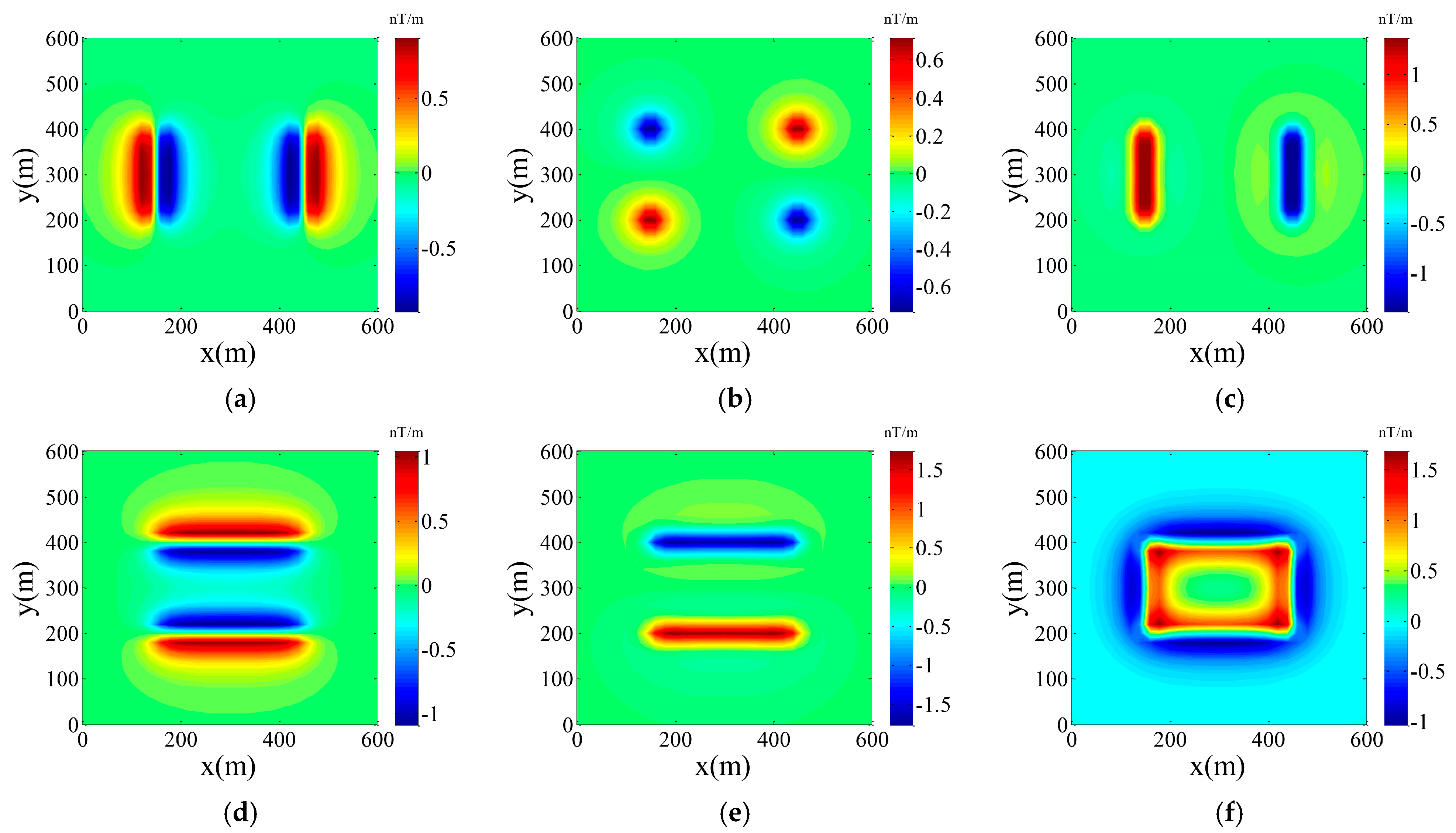
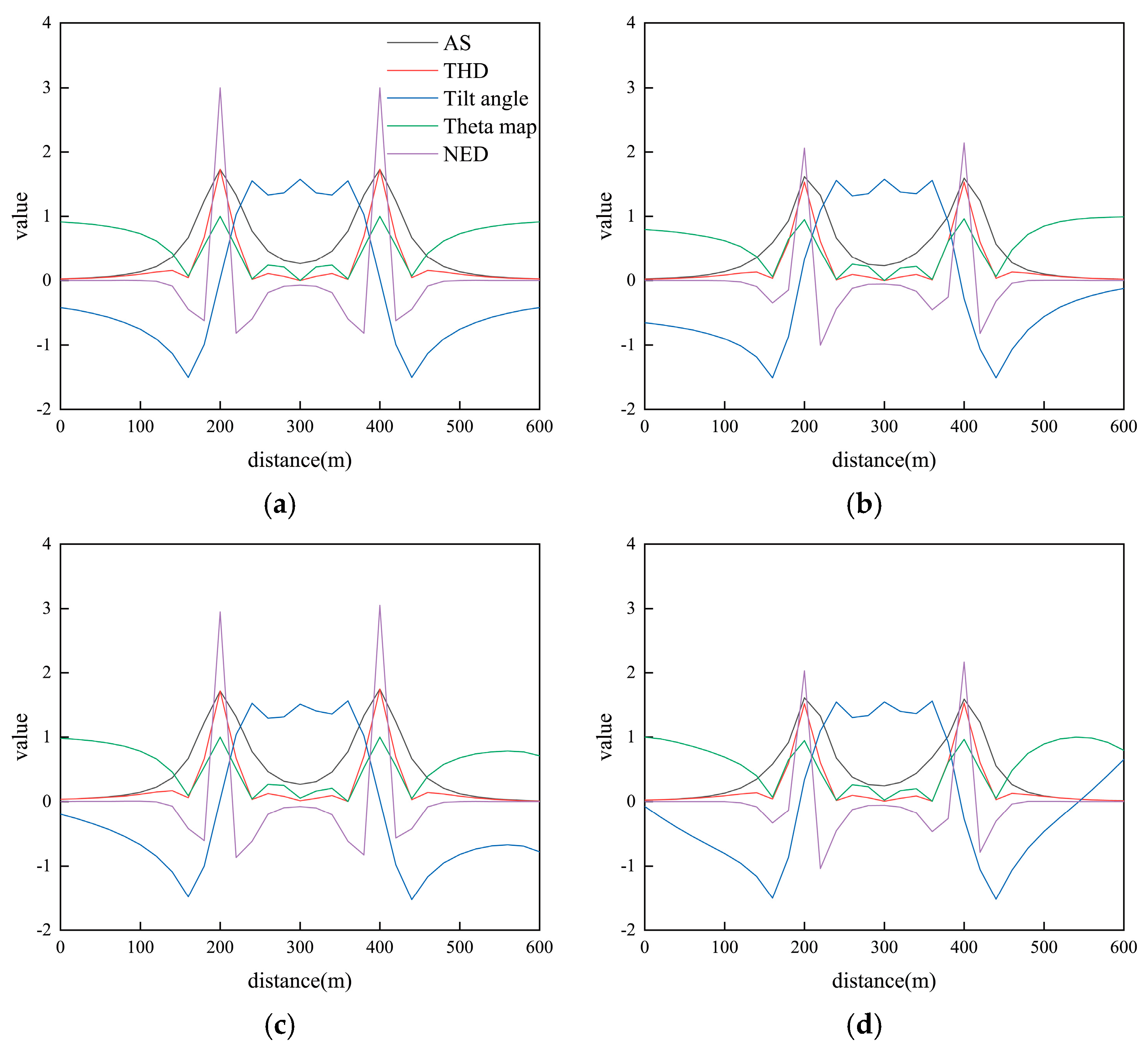
3. Edge Detection Simulation

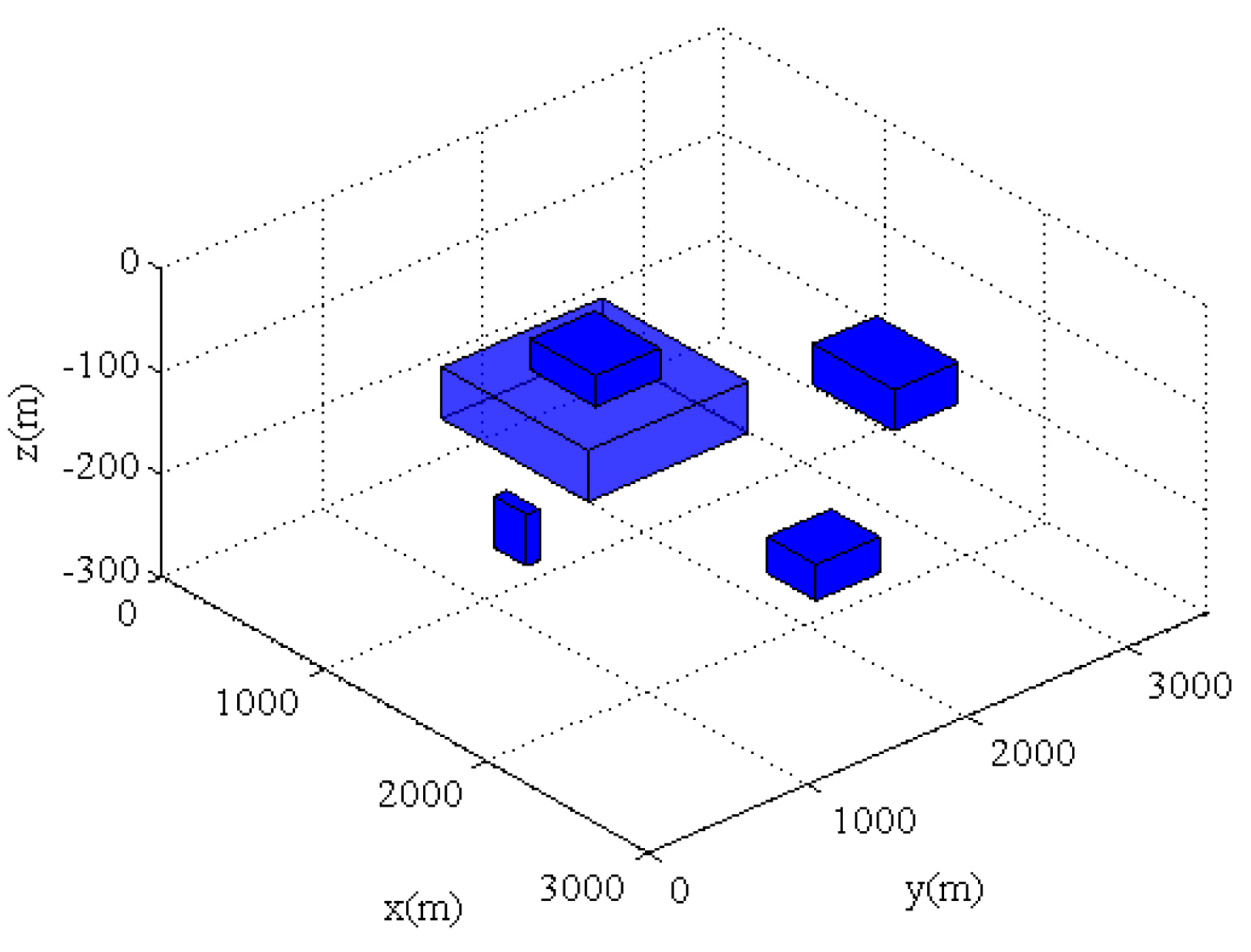
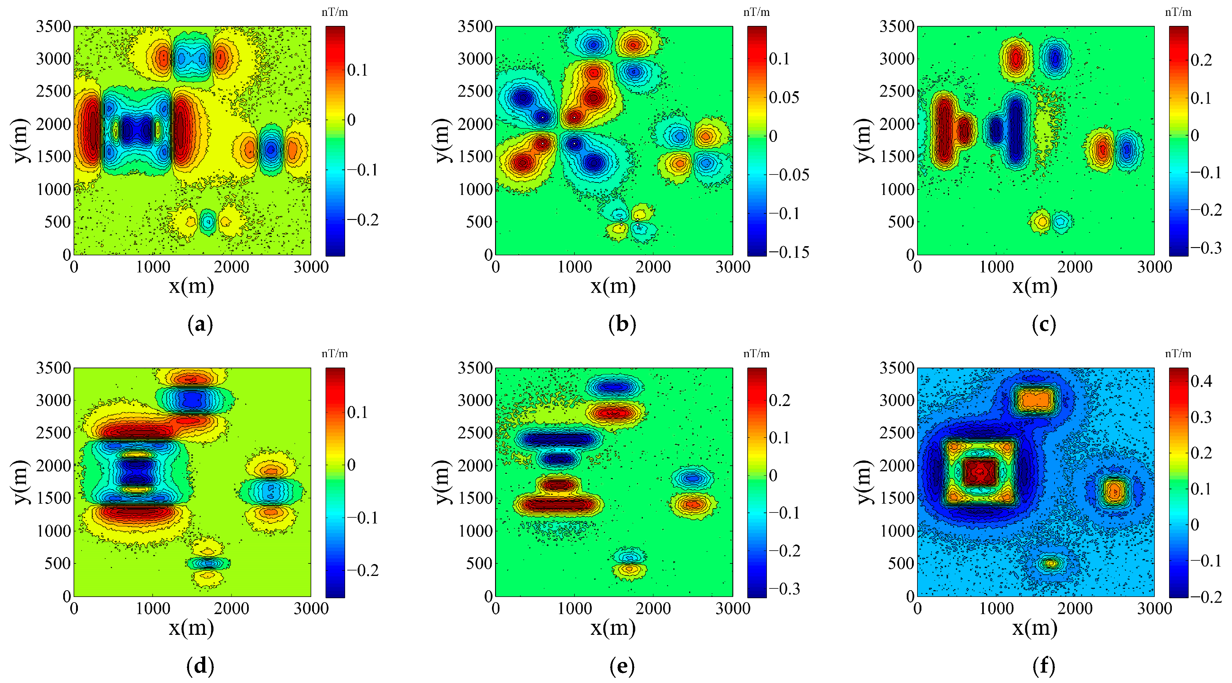
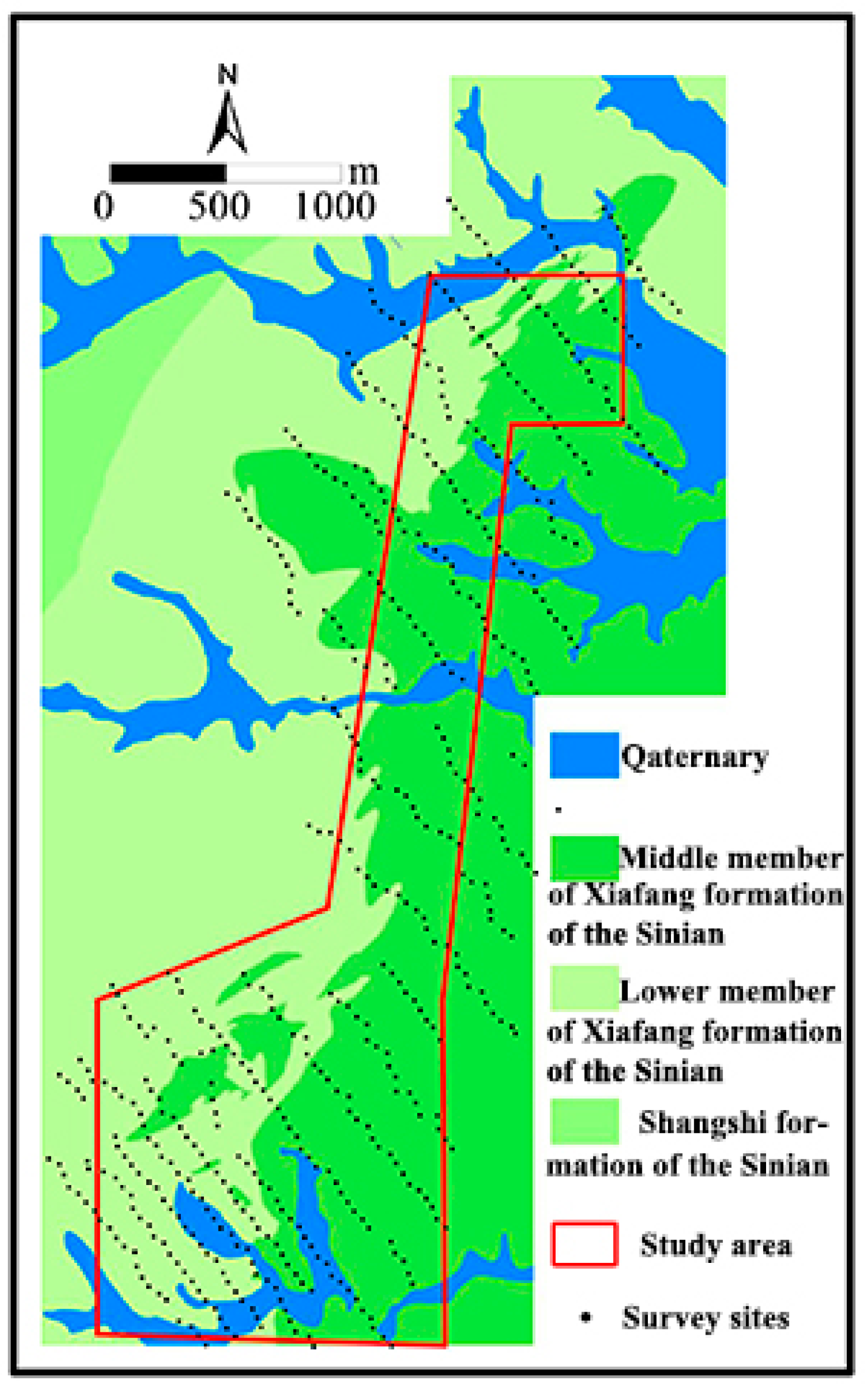
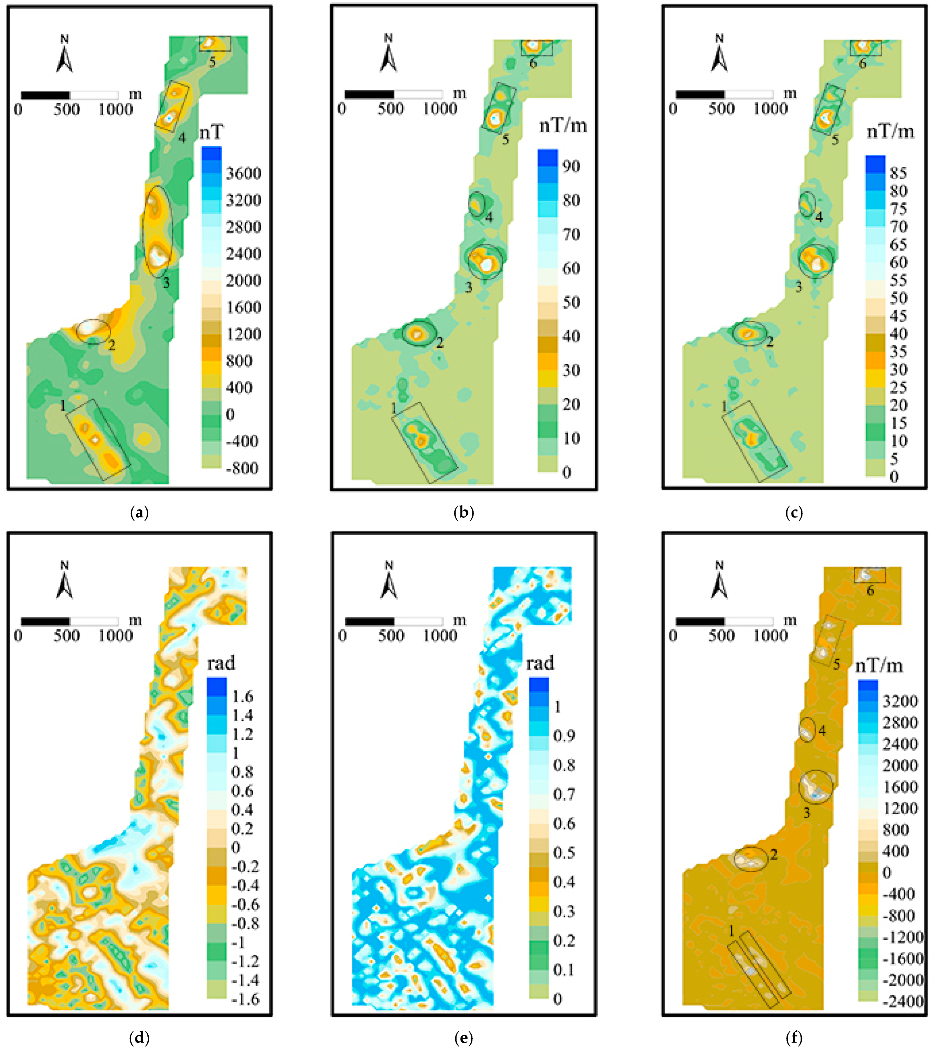
To visualize the results of several edge detection methods, the rectangle model in Table 1 is simulated. Firstly, the THD_z, AS, tilt angle, theta map, and NED method are used to detect the rectangular boundary under vertical magnetization conditions. The distribution maps of the anomaly results are shown in Figure 2; each method effectively identifies the horizontal boundary position of the rectangular body. Then, the profile curves of vertical and oblique magnetization are plotted (inclination and declination of the field are set to 60°, 33.6°), and the influence of oblique magnetization and random noise with a mean value of 0 and standard deviation of 0.01 interference on the edge detection method is discussed. The results are shown in Figure 3. Oblique magnetization affects the boundary recognition results, while noise has a more pronounced impact on the theta map and tilt angle method. The NED method proposed in this paper remains relatively unaffected by noise.

However, the anomalies are usually not single in the real situation. In order to study the distribution of magnetic anomalies in the case of multi-field sources, this paper establishes a comprehensive model, as detailed in

Table 2. Physical parameters of a comprehensive model.

Parameter	Rectangle1	Rectangle2	Rectangle3	Rectangle4	Rectangle5
Center (m)	(800, 1900, 185)	(1500, 3000, 170)	(1700, 500, 135)	(2500, 1600, 157.5)	(800, 1900, 145)
Width (m)	900	500	200	300	400
Height (m)	1000	400	80	400	400
Thickness (m)	50	40	50	35	30
Susceptibility (SI)	100	100	100	100	100

. The position of anomalies is shown in Figure 4. The total horizontal derivative, analytic signal, tilt angle, theta map, and new edge detection method are used to compare the anomaly boundaries of the comprehensive model. The actual measured data usually contains noise, which comes from the surrounding environment and instruments. Therefore, the abnormal distribution of the tensor components added random noise with the mean value of 0 and standard deviation of 0.01 in the comprehensive model is first simulated, as shown in Figure 5. Then, in this paper, the edges of several anomalies are detected. The results of edge detection using several methods such as AS, THD_z, tilt angle, theta map, and NED are discussed for vertical magnetization, oblique magnetization (inclination and declination of the field are set to 45°, 15°), and noise-containing boundaries, respectively, as shown in Figure 6.

In Figure 6, (a), (d), (g), (j), and (m) are the results of edge detection through AS, THD_z, tilt angle, theta map, and NED methods under vertical magnetization conditions, respectively. The results obtained by AS, tilt angle, and theta map are subject to the obvious mutual interference of anomalous bodies, while THD_z and NED have less interfered with anomalies. However, the NED method proposed in this paper is more convergent and has a higher resolution than THD_z for the identification of magnetic source edges.

In fact, most of the data are measured under oblique magnetization conditions; therefore, it is necessary to explore the edge detection of the combined model under oblique magnetization conditions. In Figure 6, (b), (e), (h), (k), and (n) shows the results of edge identification by several methods of AS, THD_z, tilt angle, theta map, and NED under oblique magnetization conditions, respectively. Due to the influence of oblique magnetization, the distribution of anomalies in the combined model has changed, with more pronounced effects in the presence of adjacent anomalies. Among the methods used, the theta map and tilt angle are the most significantly affected, and AS is also subject to considerable interference. THD_z is less affected by oblique magnetization and adjacent anomalies, resulting in some deviation in boundary identification. Although the NED results exhibit some variations, they are affected to the least extent, and the positions of adjacent anomalous bodies remain unaltered.

However, in reality, anomaly results are not only influenced by multiple magnetic sources and oblique magnetization but also subject to noise interference from the environment and the measurement device. Therefore, noise with a mean value of 0 and a standard deviation of 0.01 on the basis of the above-mentioned was added to simulate the effects of boundary detection for the combined anomaly source model under oblique magnetization and noise conditions. In Figure 6, (c), (f), (i), (l), and (o) show the results of AS, THD_z, tilt angle, theta map, and NED for the boundary identification of the combined model under oblique magnetization and noisy conditions, respectively. Among them, the theta map and tilt angle methods are most significantly affected and have the worst effect on anomaly source boundary detection; AS and THD_z are less affected, but the boundary identification is also obviously biased; and NED has the highest resolution for the boundary identification results almost independent of noise interference.

4. Field Example

In this section, real potential field data were used to test the performance of the proposed technique on real data. The study area is located in Jiangxi Province, China. The study area is the middle section of gold, silver, precious metals, polymetals, and iron metallogenic belts in central Jiangxi Province. The iron ore layers in the study area are anticline, synclinal layered folds are produced, the secondary folds are segmented, the morphology of the fold section is more complex, and the thickness is increased. Iron ore in the study area belongs to magnetite quartzite. The mineral composition includes quartz-magnetite, with iron evenly distributed in the sample.

The outcrops in the area are the Sinian Shangshi Formation, the Xiafang Formation metamorphic rocks, and the Quaternary alluvium. The metamorphic rock series of Shangshi and Xiafang Formations are distributed in a near NE direction, with a monoclinal structure in general and a compound synclinal structure in the local area. The distribution of the Quaternary system along the low-lying areas of gullies is shown in Figure 7. According to the geology, mineral characteristics, and geophysical conditions of the mining area, the orientation of the magnetic measurement line is northeast, with the lines oriented at an azimuth of 142°. The spacing between these survey lines is determined to be 250 m, and the interval between measurement points along these lines is fixed at 50 m. To facilitate interpretation, the magnetic anomaly data were initially reduced to the pole, with the geomagnetic inclination and declination set at 40.9° and −3.5°, respectively. Subsequently, these data were transformed into magnetic gradient tensor data using the Resource Geophysical Information System (RGIS) developed by the China Geological Survey for further analysis. In the study area and the nearby local forestry enterprises, the surface magnetic noise is small. The magnetic anomaly data were then converted into magnetic gradient tensor data for calculation. The anomaly distribution is shown in Figure 8.

From the results of anomaly distribution in the study area, it can be seen that the changes in ΔT anomalies are significant and have a large range. AS and THD_z anomalies have the same distribution pattern, but the distribution changes significantly compared to ΔT anomalies. The tilt angle and theta map cannot locate the edges of the study area, thus leading to false edges in the output map. The anomaly distribution identified by the NED method aligns with the patterns observed in ΔT anomalies, AS, and THD_z. However, it features a pronounced anomaly peak in the central region of the study area, with lower intensities towards the southern and northern extents. Anomaly distribution is more independent, and the southern anomaly is distributed in two bands.

The magnetic anomaly distribution delineates five anomalous regions from north to south, and the AS, THD_z, and NED anomaly distributions based on the magnetic gradient tensor delineate six anomalous areas from north to south. However, the tile angle and Theta map exception results are not satisfactory. In the anomaly distribution diagram, ΔT, AS, and THD_z are positive anomalies, and the convergence of the boundary of ΔT is worse than that of AS and THD_z. At the same time, anomalies No. 2, No. 3, and No. 4 in AS and THDz are obviously distributed, but these anomaly boundaries are connected with each other in the ΔT distribution diagram. The No. 1 of the NED method can delimit two parts of the anomaly; the six groups of anomalies are independent, and the boundary of the anomaly is obvious.

5. Discussions

It is well known that many edge detection techniques are based on magnetic gradient tensor data [39,52,53,54], mainly including derivative and phase-based two types. The core concept of this paper is to employ magnetic gradient tensor data for edge detection while concurrently conducting a comparative analysis with AS, THD_z, tilt angle, and theta map methods. This approach is further applied to process field example data for comprehensive evaluation.

The simulation of a single model shows that the edge detection results of the NED method are more converging (Figure 3), but it is not closed in the northwest and northeast corners (Figure 2e). In fact, most of the data are measured under oblique magnetization conditions; therefore, it is necessary to explore the edge detection of the combined model under oblique magnetization conditions. Therefore, the abnormal distribution of the tensor components added random noise with the mean value of 0 and standard deviation of 0.01 in the comprehensive model is first simulated, as shown in Figure 5. However, the overall influence on edge detection is not obvious in the simulation results of combination models with different burial depths (Figure 6m,n,o). Although NED results in the combined model are unsatisfactory only under oblique magnetization conditions (Figure 6n), the recognition effect is better than other methods when noise is added under oblique magnetization conditions (Figure 6o). AS and THD_z have the second-best anomaly recognition results after oblique magnetization and noise (Figure 6c,f), while tilt angle and theta map yield the worst results (Figure 6i,l). In the field example data processing results, NED, ΔT, AS, and THD_z anomalies are consistent (Figure 8a–c), but the NED anomaly range is more convergent (Figure 8f). The tilt angle and theta map are greatly affected by noise and oblique magnetization, which cannot locate the edges of the study area, thus leading to false edges in the abnormal results (Figure 8d,e).

6. Conclusions

In this paper, a new edge detection (NED) method based on magnetic gradient tensor is proposed and compared with AS, THD_z, tilt angle, and theta map methods. The effectiveness of various edge detection methods is assessed for both single and combined models under conditions of vertical magnetization, oblique magnetization, and noise conditions, respectively. From the simulation results, the following conclusions are obtained: the single rectangular anomaly and the profile curve show that the NED method has lower anomalies under oblique magnetization, but it is more convergent for edge detection, and it is not sensitive to noise interference. In complex scenarios with multiple anomaly bodies, simulation results indicate that the NED method’s boundary recognition remains unaffected by multiple source fields, and noise has a minimal impact. It shows strong resistance to interference and offers higher resolution. In the field example data processing results, NED, ΔT, AS, and THD_z anomalies are consistent, but the NED anomaly range is more convergent. These results also indicate that the NED algorithm is an effective method. However, the NED method proposed in this paper exhibits limited capability in recognizing the boundaries of small anomalies, and further improvements are needed in future research.

References

1. Gao, X.; Yan, S.; Li, B. A Novel Method of Localization for Moving Objects with an Alternating Magnetic Field. Sensors 2017, 17, 923. [Google Scholar] [CrossRef] [PubMed]
2. Rong, S.; Wu, J.; Liu, J.; Li, Q.; Ren, C.; Cao, X. Environmental Magnetic Characteristics and Heavy Metal Pollution Assessment of Sediments in the Le’an River, China. Minerals 2023, 13, 145. [Google Scholar] [CrossRef]
3. Ding, X.; Li, Y.; Luo, M.; Chen, J.; Li, Z.; Liu, H. Estimating Locations and Moments of Multiple Dipole-Like Magnetic Sources From Magnetic Gradient Tensor Data Using Differential Evolution. IEEE Trans. Geosci. Remote Sens. 2022, 60, 5904913. [Google Scholar] [CrossRef]
4. Xu, L.; Gu, H.; Chang, M.; Fang, L.; Lin, P.; Lin, C. Magnetic Target Linear Location Method Using Two-Point Gradient Full Tensor. IEEE Trans. Instrum. Meas. 2021, 70, 6007808. [Google Scholar] [CrossRef]
5. Xu, L.; Huang, X.; Dai, Z.; Yuan, F.; Wang, X.; Fan, J. Blind Spots Analysis of Magnetic Tensor Localization Method. Remote Sens. 2023, 15, 2199. [Google Scholar] [CrossRef]
6. Wynn, W.; Frahm, C.; Carroll, P.; Clark, R.; Wellhoner, J.; Wynn, M. Advanced Superconducting Gradiometer/Magnetometer Arrays and a Novel Signal Processing Technique. IEEE Trans. Magn. 1975, 11, 701–707. [Google Scholar] [CrossRef]
7. Chwala, A.; Stolz, R.; Zakosarenko, V.; Fritzsch, L.; Schulz, M.; Rompel, A.; Polome, L.; Meyer, M.; Meyer, H.G. Full Tensor SQUID Gradiometer for Airborne Exploration. ASEG Ext. Abstr. 2012, 2012, 1–4. [Google Scholar] [CrossRef]
8. Schmidt, P.; Clark, D.; Leslie, K.; Bick, M.; Tilbrook, D.; Foley, C. GETMAG—A SQUID Magnetic Tensor Gradiometer for Mineral and Oil Exploration. Explor. Geophys. 2004, 35, 297–305. [Google Scholar] [CrossRef]
9. Stolz, R.; Fritzsch, L.; Meyer, H.-G. LTS SQUID Sensor with a New Configuration. Supercond. Sci. Technol. 1999, 12, 806–808. [Google Scholar] [CrossRef]
10. Schiffler, M.; Queitsch, M.; Stolz, R.; Chwala, A.; Krech, W.; Meyer, H.-G.; Kukowski, N. Calibration of SQUID Vector Magnetometers in Full Tensor Gradiometry Systems. Geophys. J. Int. 2014, 198, 954–964. [Google Scholar] [CrossRef]
11. Schmidt, P.; Clark, D. Advantages of Measuring the Magnetic Gradient Tensor. Preview 2000, 85, 26–30. [Google Scholar]
12. Schmidt, P.W.; Clark, D.A. The Magnetic Gradient Tensor: Its Properties and Uses in Source Characterization. Lead. Edge 2006, 25, 75–78. [Google Scholar] [CrossRef]
13. Clark, D.A. Corrigendum to: New Methods for Interpretation of Magnetic Vector and Gradient Tensor Data I: Eigenvector Analysis and the Normalised Source Strength. Explor. Geophys. 2014, 45, 267–282. [Google Scholar] [CrossRef]
14. Yin, G.; Zhang, L.; Jiang, H.; Wei, Z.; Xie, Y. A Closed-Form Formula for Magnetic Dipole Localization by Measurement of Its Magnetic Field Vector and Magnetic Gradient Tensor. J. Magn. Magn. Mater. 2020, 499, 166274. [Google Scholar] [CrossRef]
15. Lin, S.; Pan, D.; Wang, B.; Liu, Z.; Liu, G.; Wang, L.; Li, L. Improvement and Omnidirectional Analysis of Magnetic Gradient Tensor Invariants Method. IEEE Trans. Ind. Electron. 2021, 68, 7603–7612. [Google Scholar] [CrossRef]
16. Xu, L.; Zhang, N.; Fang, L.; Lin, P.; Chen, H.; Chang, M. Error Analysis of Cross-Shaped Magnetic Gradient Full Tensor Measurement System. AIP Adv. 2020, 10, 125201. [Google Scholar] [CrossRef]
17. Nabighian, M.N. The analytic signal of two-dimensional magnetic bodies with polygonal cross-section: Its properties and use for automated anomaly interpretation. Geophysics 1972, 37, 507–517. [Google Scholar] [CrossRef]
18. Roest, W.R.; Verhoef, J.; Pilkington, M. Magnetic Interpretation Using the 3-D Analytic Signal. Geophysics 1992, 57, 116–125. [Google Scholar] [CrossRef]
19. Qin, S. An Analytic Signal Approach to the Interpretation of Total Field Magnetic Anomalies. Geophys. Prospect. 1994, 42, 665–675. [Google Scholar] [CrossRef]
20. Nabighian, M.N. Toward a Three-dimensional Automatic Interpretation of Potential Field Data via Generalized Hilbert Transforms: Fundamental Relations. Geophysics 1984, 49, 780–786. [Google Scholar] [CrossRef]
21. Beiki, M. Analytic Signals of Gravity Gradient Tensor and Their Application to Estimate Source Location. Geophysics 2010, 75, I59–I74. [Google Scholar] [CrossRef]
22. Yuan, Y.; Yu, Q. Edge Detection in Potential-Field Gradient Tensor Data by Use of Improved Horizontal Analytical Signal Methods. Pure Appl. Geophys. 2015, 172, 461–472. [Google Scholar] [CrossRef]
23. Yuan, Y.; Geng, M. Directional Total Horizontal Derivatives of Gravity Gradient Tensor and Their Application to Delineat the Edges. In Proceedings of the 76th EAGE Conference & Exhibition, Amsterdam, The Netherlands, 16–19 June 2014. [Google Scholar] [CrossRef]
24. Miller, H.G.; Singh, V. Potential Field Tilt—A New Concept for Location of Potential Field Sources. J. Appl. Geophys. 1994, 32, 213–217. [Google Scholar] [CrossRef]
25. Li, Q.; Li, Z.; Shi, Z.; Fan, H. Application of Helbig Integrals to Magnetic Gradient Tensor Multi-Target Detection. Measurement 2022, 200, 111612. [Google Scholar] [CrossRef]
26. Gang, Y.; Yingtang, Z.; Hongbo, F.; Zhining, L.; Guoquan, R. Detection, Localization and Classification of Multiple Dipole-like Magnetic Sources Using Magnetic Gradient Tensor Data. J. Appl. Geophys. 2016, 128, 131–139. [Google Scholar] [CrossRef]
27. Ferreira, F.J.F.; de Souza, J.; de B. e S. Bongiolo, A.; de Castro, L.G. Enhancement of the Total Horizontal Gradient of Magnetic Anomalies Using the Tilt Angle. Geophysics 2013, 78, J33–J41. [Google Scholar] [CrossRef]
28. Verduzco, B.; Fairhead, J.D.; Green, C.M.; MacKenzie, C. New Insights into Magnetic Derivatives for Structural Mapping. Lead. Edge 2004, 23, 116–119. [Google Scholar] [CrossRef]
29. Wijns, C.; Perez, C.; Kowalczyk, P. Theta Map: Edge Detection in Magnetic Data. Geophysics 2005, 70, L39–L43. [Google Scholar] [CrossRef]
30. Eldosouky, A.M.; Mohamed, H. Edge Detection of Aeromagnetic Data as Effective Tools for Structural Imaging at Shilman Area, South Eastern Desert, Egypt. Arab. J. Geosci. 2021, 14, 13. [Google Scholar] [CrossRef]
31. Ma, G.; Li, L. Edge Detection in Potential Fields with the Normalized Total Horizontal Derivative. Comput. Geosci. 2012, 41, 83–87. [Google Scholar] [CrossRef]
32. Oruç, B. Location and Depth Estimation of Point-Dipole and Line of Dipoles Using Analytic Signals of the Magnetic Gradient Tensor and Magnitude of Vector Components. J. Appl. Geophys. 2010, 70, 27–37. [Google Scholar] [CrossRef]
33. Li, J.; Zhang, Y.; Fan, H.; Li, Z. Preprocessed Method and Application of Magnetic Gradient Tensor Data. IEEE Access 2019, 7, 173738–173752. [Google Scholar] [CrossRef]
34. Li, G.; Liu, S.; Shi, K.; Hu, X. Normalized Edge Detectors Using Full Gradient Tensors of Potential Field. Pure Appl. Geophys. 2023, 180, 2327–2349. [Google Scholar] [CrossRef]
35. Beiki, M.; Clark, D.A.; Austin, J.R.; Foss, C.A. Estimating Source Location Using Normalized Magnetic Source Strength Calculated from Magnetic Gradient Tensor Data. Geophysics 2012, 77, J23–J37. [Google Scholar] [CrossRef]
36. Phillips, J.D.; Nabighian, M.N.; Smith, D.V.; Li, Y. Estimating Locations and Total Magnetization Vectors of Com-pact Magnetic Sources from Scalar, Vector, or Tensor Magnetic Measurements through Combined Helbig and Euler Analysis. In SEG Technical Program Expanded Abstracts 2007; Society of Exploration Geophysicists: Houston, TX, USA, 2007; pp. 770–774. [Google Scholar] [CrossRef]
37. Salem, A.; Ravat, D. A Combined Analytic Signal and Euler Method (AN-EUL) for Automatic Interpretation of Magnetic Data. Geophysics 2003, 68, 1952–1961. [Google Scholar] [CrossRef]
38. Ji, S.; Zhang, H.; Wang, Y.; Rong, L.; Shi, Y.; Chen, Y. Three-dimensional Inversion of Full Magnetic Gradient Tensor Data Based on Hybrid Regularization Method. Geophys. Prospect. 2019, 67, 226–261. [Google Scholar] [CrossRef]
39. Prasad, K.N.D.; Pham, L.T.; Singh, A.P.; Eldosouky, A.M.; Abdelrahman, K.; Fnais, M.S.; Gómez-Ortiz, D. A Novel Enhanced Total Gradient (ETG) for Interpretation of Magnetic Data. Minerals 2022, 12, 1468. [Google Scholar] [CrossRef]
40. Pham, L.T.; Oksum, E.; Vu, M.D.; Vo, Q.T.; Du Le-Viet, K.; Eldosouky, A.M. An Improved Approach for Detecting Ridge Locations to Interpret the Potential Field Data for More Accurate Structural Mapping: A Case Study from Vredefort Dome Area (South Africa). J. Afr. Earth Sci. 2021, 175, 104099. [Google Scholar] [CrossRef]
41. Eldosouky, A.M.; Pham, L.T.; Henaish, A. High Precision Structural Mapping Using Edge Filters of Potential Field and Remote Sensing Data: A Case Study from Wadi Umm Ghalqa Area, South Eastern Desert, Egypt. Egypt. J. Remote Sens. Space Sci. 2022, 25, 501–513. [Google Scholar] [CrossRef]
42. Eldosouky, A.M.; Pham, L.T.; Duong, V.-H.; Kemgang Ghomsi, F.E.; Henaish, A. Structural Interpretation of Potential Field Data Using the Enhancement Techniques: A Case Study. Geocarto Int. 2022, 37, 16900–16925. [Google Scholar] [CrossRef]
43. Ekwok, S.E.; Eldosouky, A.M.; Ben, U.C.; Achadu, O.-I.M.; Akpan, A.E.; Othman, A.; Pham, L.T. An Integrated Approach of Advanced Methods for Mapping Geologic Structures and Sedimentary Thickness in Ukelle and Adjoining Region (Southeast Nigeria). Earth Sci. Res. J. 2023, 27, 251–258. [Google Scholar] [CrossRef]
44. Thanh Pham, L.; Anh Nguyen, D.; Eldosouky, A.M.; Abdelrahman, K.; Van Vu, T.; Al-Otaibi, N.; Ibrahim, E.; Kharbish, S. Subsurface Structural Mapping from High-Resolution Gravity Data Using Advanced Processing Methods. J. King Saud Univ.-Sci. 2021, 33, 101488. [Google Scholar] [CrossRef]
45. Thanh Pham, L.; Eldosouky, A.M.; Melouah, O.; Abdelrahman, K.; Alzahrani, H.; Oliveira, S.P.; Andráš, P. Mapping Subsurface Structural Lineaments Using the Edge Filters of Gravity Data. J. King Saud Univ.-Sci. 2021, 33, 101594. [Google Scholar] [CrossRef]
46. Eldosouky, A.M.; Elkhateeb, S.O.; Mahdy, A.M.; Saad, A.A.; Fnais, M.S.; Abdelrahman, K.; Andráš, P. Structural Analysis and Basement Topography of Gabal Shilman Area, South Eastern Desert of Egypt, Using Aeromagnetic Data. J. King Saud Univ.-Sci. 2022, 34, 101764. [Google Scholar] [CrossRef]
47. Eldosouky, A.M.; Pham, L.T.; Abdelrahman, K.; Fnais, M.S.; Gomez-Ortiz, D. Mapping Structural Features of the Wadi Umm Dulfah Area Using Aeromagnetic Data. J. King Saud Univ.-Sci. 2022, 34, 101803. [Google Scholar] [CrossRef]
48. Li, Q.; Li, Z.; Shi, Z.; Fan, H. Multi-Target Magnetic Positioning Using SAFCM Clustering and Invariants-Improved Tilt Angle. IEEE Trans. Geosci. Remote Sens. 2022, 60, 5924015. [Google Scholar] [CrossRef]
49. Li, Q.; Li, Z.; Shi, Z.; Fan, H. Magnetic Object Recognition with Magnetic Gradient Tensor System Heading-Line Surveys Based on Kernel Extreme Learning Machine and Sparrow Search Algorithm. Measurement 2022, 203, 111967. [Google Scholar] [CrossRef]
50. Deng, H.; Hu, X.; Cai, H.; Liu, S.; Peng, R.; Liu, Y.; Han, B. 3D Inversion of Magnetic Gradient Tensor Data Based on Convolutional Neural Networks. Minerals 2022, 12, 566. [Google Scholar] [CrossRef]
51. Luo, Y.; Wu, M.-P.; Wang, P.; Duan, S.-L.; Liu, H.-J.; Wang, J.-L.; An, Z.-F. Full Magnetic Gradient Tensor from Triaxial Aeromagnetic Gradient Measurements: Calculation and Application. Appl. Geophys. 2015, 12, 283–291. [Google Scholar] [CrossRef]
52. Prasad, K.N.D.; Pham, L.T.; Singh, A.P. Structural Mapping of Potential Field Sources Using BHG Filter. Geocarto Int. 2022, 37, 11253–11280. [Google Scholar] [CrossRef]
53. Prasad, K.N.D.; Pham, L.T.; Singh, A.P. A Novel Filter “ImpTAHG” for Edge Detection and a Case Study from Cambay Rift Basin, India. Pure Appl. Geophys. 2022, 179, 2351–2364. [Google Scholar] [CrossRef]
54. Chen, T.; Zhang, G. NHF as an Edge Detector of Potential Field Data and Its Application in the Yili Basin. Minerals 2022, 12, 149. [Google Scholar] [CrossRef]
Figure 1. Five independent and vertical components of the magnetic gradient tensor of the rectangle: (a) Bxx; (b) Bxy; (c) Bxz; (d) Byy; (e) Byz; (f) Bzz.
Minerals 14 00657 g001
Figure 2. Single rectangle edge detection results of different methods: (a) AS; (b) THDz; (c) tilt angle; (d) theta map; (e) NED.
Minerals 14 00657 g002
Figure 3. Profile curves of different edge detection methods at x = 300m profile: (a) noise-free vertical magnetization; (b) noise-free oblique magnetization; (c) noise-corrupted vertical magnetization; (d) noise-corrupted oblique magnetization.
Minerals 14 00657 g003
Figure 4. Simulation model of positioning rectangles.
Minerals 14 00657 g004
Figure 5. Simulated five independent components of magnetic gradient tensor of the four rectangles, including noise: (a) Bxx; (b) Bxy; (c) Bxz; (d) Byy; (e) Byz; (f) Bzz.
Minerals 14 00657 g005
Figure 6. Five prisms edge detection results of different methods. Results of vertical magnetization: (a) AS; (d) THDz; (g) tilt angle; (j) theta map; (m) NED. Results of oblique magnetization: (b) AS; (e) THDz; (h) tilt angle; (k) theta map; (n) NED. Results of oblique magnetization and noise: (c) AS; (f) THDz; (i) tilt angle; (l) theta map; (o) NED. The blue lines show the true edge of the prisms.
Minerals 14 00657 g006aMinerals 14 00657 g006b
Figure 7. The geology of the study area.
Minerals 14 00657 g007
Figure 8. Anomaly distribution map of the study area: (a) ΔT; (b) AS; (c) THDz; (d) tilt angle; (e) theta map; (f) NED.
Minerals 14 00657 g008