Data-Driven Classification and Logging Prediction of Mudrock Lithofacies Using Machine Learning: Shale Oil Reservoirs in the Eocene Shahejie Formation, Bonan Sag, Bohai Bay Basin, Eastern China

Abstract

As the world’s energy demand continues to expand, shale oil has a substantial influence on the global energy reserves. The third submember of the Mbr 3 of the Shahejie Fm, characterized by complicated mudrock lithofacies, is one of the significant shale oil enrichment intervals of the Bohai Bay Basin. The classification and identification of lithofacies are key to shale oil exploration and development. However, the efficiency and reliability of lithofacies identification results can be compromised by qualitative classification resulting from an incomplete workflow. To address this issue, a comprehensive technical workflow for mudrock lithofacies classification and logging prediction was designed based on machine learning. Principal component analysis (PCA) and hierarchical cluster analysis (HCA) were conducted to realize the automatic classification of lithofacies, which can classify according to the internal relationship of the data without the disturbance of human factors and provide an accurate lithofacies result in a much shorter time. The PCA and HCA results showed that the third submember can be split into five lithofacies: massive argillaceous limestone lithofacies (MAL), laminated calcareous claystone lithofacies (LCC), intermittent lamellar argillaceous limestone lithofacies (ILAL), continuous lamellar argillaceous limestone lithofacies (CLAL), and laminated mixed shale lithofacies (LMS). Then, random forest (RF) was performed to establish the identification model for each of the lithofacies and the obtained model is optimized by grid search (GS) and K-fold cross validation (KCV), which could then be used to predict the lithofacies of the non-coring section, and the three validation methods showed that the accuracy of the GS–KCV–RF model were all above 93%. It is possible to further enhance the performance of the models by resampling, incorporating domain knowledge, and utilizing the mechanism of attention. Our method solves the problems of the subjective and time-consuming manual interpretation of lithofacies classification and the insufficient generalization ability of machine-learning methods in the previous works on lithofacies prediction research, and the accuracy of the model for mudrocks lithofacies prediction is also greatly improved. The lithofacies machine-learning workflow introduced in this study has the potential to be applied in the Bohai Bay Basin and comparable reservoirs to enhance exploration efficiency and reduce economic costs.

1. Introduction

Lithofacies are inherent properties of rocks or rock combinations formed under certain sedimentary conditions that reflect specific processes or environments. Lithofacies can reflect the sedimentary environment for facies analysis, and determine the fundamental properties of subsurface reservoirs [1,2,3,4]. Determining the lithofacies type and distribution is critical for shale oil exploration and development [5,6]. Mudrock (grain size < 63 μm) lithofacies related to shale oil (gas) is a comprehensive representation of mineral composition, organic matter content, grain size, and structural characteristics. The determination of mudrock lithofacies necessitates manual interpretation based on core observations, scanning electron microscopy (SEM), and X-ray diffraction (XRD) analysis [7,8,9,10,11,12,13,14], which is usually time-consuming, labor-intensive, and subjective. PCA and HCA, unsupervised machine-learning algorithms, can automatically classify according to the similarity of samples without prior classification [15]. PCA and HCA can automatically classify lithofacies utilizing known petrological and petrophysical properties within a specific area, to streamline decision-making processes and increase efficiency in lithofacies classification.

The analysis of lithofacies distribution is limited by the high cost of coring. Logging data provide a cost-effective and time-efficient alternative to core analysis, as it encompasses various petrological parameters that can accurately characterize the physical characters of the subsurface rock formation. As a result, the utilization of well logs for lithofacies identification has gained considerable popularity [16,17,18,19]. Various mathematical techniques have been implemented to train lithofacies identification models using labeled logging data, and machine-learning algorithms perform well [20,21,22]. These algorithms include linear discriminant analysis (LDA) [22,23,24], naïve Bayes (NB) [25,26], decision trees (DTs) [20,27,28], support vector machines (SVMs) [29,30,31], artificial neural networks (ANNs)] [32,33,34], extreme gradient boosting (XGBoost) [28,35], random forest (RF) [20,28,36], etc. Tewari and Dwivedi used ensemble methods to identify the lithofacies of a Kansas (U.S.A.) oilfield with an average accuracy of 85% [37]. A deep residual convolutional network was applied to classify four lithofacies in a Brazilian pre-salt oilfield and the accuracy is 81.45% [38]. For the Marcellus and Bakken Shale of the United States, ANN, SVM, self-organizing map (SOM), and multi-resolution graph-based clustering (MRGC) were used to build quantitative lithofacies modeling, and the overall accuracy is about 80% [39,40]. Few of these studies focused on lacustrine mudrock and shale reservoirs, and the accuracy of lithofacies identification is relatively low. RF is an ensemble analysis method based on decision trees with a higher precision and generalization ability than a single classifier [27,28]. The application of RF to the lithofacies identification of lacustrine mudrock has great significance.

This study aims to apply the machine-learning-based approach to lacustrine mudrock lithofacies classification and prediction using petrological parameters and conventional logging data. We achieved the quantitative classification of mudrock lithofacies by PCA and HCA methods. PCA and HCA offers the benefit of utilizing the internal data relationship without the disturbance of human factors to determine lithofacies, resulting in a significantly reduced time while ensuring the precision of lithofacies classification. In addition, we used optimized RF to predict the lithofacies of the non-coring section by adopting grid search (GS) and K-fold cross validation (KCV) to optimize the parameters of the RF algorithm for higher accuracy. Unlike prior research that focused on overall accuracy, this study conducted a comprehensive evaluation of each lithofacies class, considering multiple metrics, and the performance, improvement, and application of machine-learning models were proposed. This study establishes a comprehensive workflow for the automatic classification and prediction of mudrock lithofacies based on more efficient and precise machine-learning algorithms, which can deepen the application of machine-learning methods in the geological field and improve the efficiency of shale oil exploration.

2. Geological Setting

Covering an expansive area of more than 600 km², the Bonan Sag is the largest secondary negative tectonic unit in the middle of the Zhanhua Sag of the Jiyang Depression in Bohai Bay Basin, eastern China (Figure 1a,b). It stands out as a sag with a remarkable depth of burial within the Jiyang Depression and has the best accumulation conditions. The Bonan Sag includes a series of NW–SE and NE–SW trending faults that are mainly derived from the Yanshan and Himalayan movements [41]. The Sag is bordered by the Chengdong Uplift in the north, Yihezhuang Uplift in the west, Chenjiazhuang Uplift in the south, and Gudao Uplift in the east. From south to north, the Bonan Sag exhibits a subdivision into four tectonic zones: the Southern Gentle Slope Zone, Boshen4 Step-Fault Zone, Bonan Deep Sag Zone, and Northern Steep Slope Zone, presenting with a narrow strip shape (Figure 1c) [42,43].

The Bonan Sag is a Meso-Cenozoic faulted depression overlying the Paleozoic basement of the North China Craton [44]. Dividing the Cenozoic based on the distribution of regional unconformities reveals the existence of two distinct tectonic sequences [22]. Comprising fluvial–lacustrine sediments, the lower group is the syn-rift tectonic sequence and is composed of the Paleogene Kongdian, Shahejie, and Dongying formations. The subsequent post-rift tectonic sequence comprises coarse clastic fluvial sediments, including the Neogene Guantao and Minghuazhen formations, and the Quaternary Pingyuan Formation [45]. The Shahejie Formation is divided into four members from bottom to top: Es₄, Es₃, Es₂, and Es₁. The Es₄ and Es₃ are the major layers for shale oil exploration and can be further divided into two and three submembers, respectively (Figure 2) [41].

The Bonan Sag has good reservoir-forming conditions. The third submember of the Mbr 3 of the Shahejie Fm holds significant importance as one of the most organic-rich layers and is extensively distributed in the Bonan Sag, with a thickness of 300–500 m [22]. During the third submember deposition stage, the basement subsided rapidly, forming a sustained deep lacustrine and brackish water environment in a warm climate (Figure 2). The dominant lithological components of the third submember include dark gray claystone and calcareous claystone and gray-brown shale with claystone intercalations, and many carbonate minerals are present as laminae interlayered within claystone or shale layers [8,42].

3. Samples and Methods

3.1. Data

3.1.1. Core Samples

The observation and sampling of conventional cores from 8 wells were conducted at the Drill Core Store of the Shengli Oilfield Company of the SINOPEC Group. These wells exhibited an abundance of organic-rich shale and mudstone, with coring intervals uniformly belong to the Es3³ member. First, 214 samples were obtained from the coring intervals of wells L69, which were primarily utilized for thin-section observations, X-ray diffraction (XRD) analysis. Then, 42 microarea samples were collected for M-TOC analysis. A total of 266 bulk TOC, 197 porosity, 208 permeability, and 199 oil saturation data points were collected from the Geological Scientific Research Institute of the China Sinopec Shengli Oilfield Company (

Table 1. The statistics of testing results.

Statistical Information	Bulk TOC (%)	Porosity (%)	Permeability (mD)	So	XRD Results			M-TOC (%)
					Clay (%)	Carb (%)	Felsic (%)
N	266	197	208	199	214	214	214	42
mean	2.9	4.8	4.5	62.7	19	57	20	7.3
min	0.5	1.3	0.1	27.8	4	12	5	0.6
25%	1.7	3.2	0.6	52.5	12	49	16	3.6
50%	2.7	4.6	1.9	60.7	18	58	19	5.2
75%	3.7	6.1	10.1	73.3	24	66	22	10.2
max	9.3	10.4	75.3	97.2	48	89	45	22.4

Carb is short for carbonate minerals = calcite + dolomite; Felsic is short for felsic terrigenous clastic minerals = quartz + plagioclase + K-feldspar; So is short for oil saturation.

).

3.1.2. Thin Sections

Thin sections of all core samples were manufactured at Resources Exploration Laboratory of China University of Geosciences, Beijing. The procedure of the thin sections production involved several steps: sample cutting (25 × 25 × 3 mm), polishing, gluing with epoxy, grind to thickness of 0.03 mm, and repolishing. Thin sections observation was performed at Leica DM2500P.

3.1.3. X-Ray Diffraction

X-ray diffraction (XRD) was performed on 214 samples for quantitative analysis of the mineral composition using a D/max-2500 TTR system at the China Sinopec Shengli Oilfield Company. The instrument operated at a tube pressure of 30 kV, a conduit flow of 40 mA, and a scanning speed of 20/min. The results of XRD analysis were shown in Table 1.

3.1.4. Microdomain TOC

Microdomain TOC (M-TOC) was utilized to evaluate the TOC of different lithofacies, ensuring that carbonate minerals did not mix with the claystone samples. Sampling was performed by cutting and polishing 5 × 3 × 1 cm blocks from the samples. The M-TOC data were measured utilizing a Multi NC2100S carbon-sulfur instrument and following the Chinese National Standard method GB/T 19, 145–2003 [8] at the Laboratory of Geological Microbiology of China University of Geosciences, Beijing (Table 1).

3.1.5. Logging Data

Conventional logging data from 6 wells in the Bonan Sag were analyzed to determine the sensitive parameters of the lithofacies and establish a logging identification model. A total of eight well log types were selected: caliper (CAL), natural gamma ray (GR), density (DEN), compensated neutron (CNL), acoustic velocity (AC), spontaneous potential (SP), and resistivity log (LLD and LLS). The sampling interval of the logging data was 0.125 m. Prior to the lithofacies identification, data preprocessing was performed to ensure the accuracy and reliability of the logging data: (1) Since sandstones/carbonates have lower GR values than claystone/shale, a core-to-log depth offset calibration was performed for all well logs by matching the marker spacing with the GR log; (2) Invalid values such as 9999, 999, or 0, which fails to accurately depict the true conditions of the subsurface rock formations, were removed; (3) Considering the numerical distribution of the resistivity log data, we convert LLD and LLS into LNLLD and LNLLS; (4) Linear normalization was applied to convert the raw logging data to the same magnitude (0–1) to avoid the influence of differences in the value ranges of the well logs.

3.2. Machine-Learning Algorithms

3.2.1. Principal Component Analysis (PCA)

PCA is an unsupervised multivariate statistical algorithm that reduces the dimensionality of a dataset. PCA does not require a prior weighting of data, which reduces subjectivity due to the individual viewpoints of decision makers [46,47]. It uses an orthogonal transformation to convert correlated variables into a set of linearly uncorrelated variables called principal components (PCs). PCs can replace primary multidimensional information, and their information does not overlap ensuring the minimal loss of original information [48,49]. Multiple types of petrological and geochemical parameters can be replaced by a few PCs using PCA for classifying lithofacies.

3.2.2. Hierarchical Cluster Analysis (HCA)

HCA is a popular unsupervised algorithm that aims to classify a dataset into groups based on the measurement of the similarity between groups [48,50]. HCA is suitable for datasets with arbitrary attributes and can generate a hierarchical tree that can be visualized to directly show the hierarchical relationships between classes. At the beginning of HCA, each object is classified as a separate cluster, and the distances (similarities) among all pairs of objects are computed by the Euclidean distance algorithms [51].

$$d_{rs}^2=\left(C_r-C_s\right)\left(C_r-C_s\right)’$$

(1)

The two most similar clusters are then merged into a new cluster and their distances are updated. The algorithm stops when all the objects merge into a single cluster [51,52].

3.2.3. Random Forest (RF)

RF is an ensemble analysis method based on decision trees (DTs) and bagging. RF generates multiple decision trees by utilizing a predefined variable number for splitting at each decision tree and bagging node, employing a randomly subsetting algorithm [53]. Each tree has different training sets and randomly selected features determined by cross-validation. Compared with the decision tree, the RF employs a different strategy for feature selection during each split process. For the classification problem, RF predicts classes based on majority votes [54]. Additionally, RF can assess the importance of each feature and evaluate their role in the classification by providing an importance score [55].

3.2.4. Grid Search (GS)–K-Fold Cross Validation (KCV)–Random Forest (RF)

The main control parameters of RF include the number of DTs, the maximum tree depth, and the number of features when the tree splits. The accuracy of the RF classification model can be enhanced by utilizing grid search (GS) and K-fold cross validation (KCV) to select the optimal parameters. The GS method, an exhaustive search method, is one of the most commonly used algorithms to determine optimal hyperparameters [56]. The basic principle of GS is to explore the hyperparameters within the designated range, and adjust the model parameters based on the step length. Starting from the minimum value, the hyperparameter is incremented by the step length until it surpasses the maximum value in the designated range. Subsequently, the adjusted parameters are utilized to train the learners and search for the optimal combination of hyperparameters that yields the highest accuracy on the testing set. KCV can produce the evaluation index for the model by partitioning the training set into K uniform-sized portions [57]. K models are built by taking each portion of the training set as the validation set and the surplus K − 1 portions as the new training set. According to the average precision of K models, the performance of RF classifier model is assessed. Following this, the parameters of the RF are adjusted using the GS method, resulting in the recalculation of the precision of it. By comparing the precisions of the RF models across various parameter combinations, the optimal parameter combination for the classifier is determined.

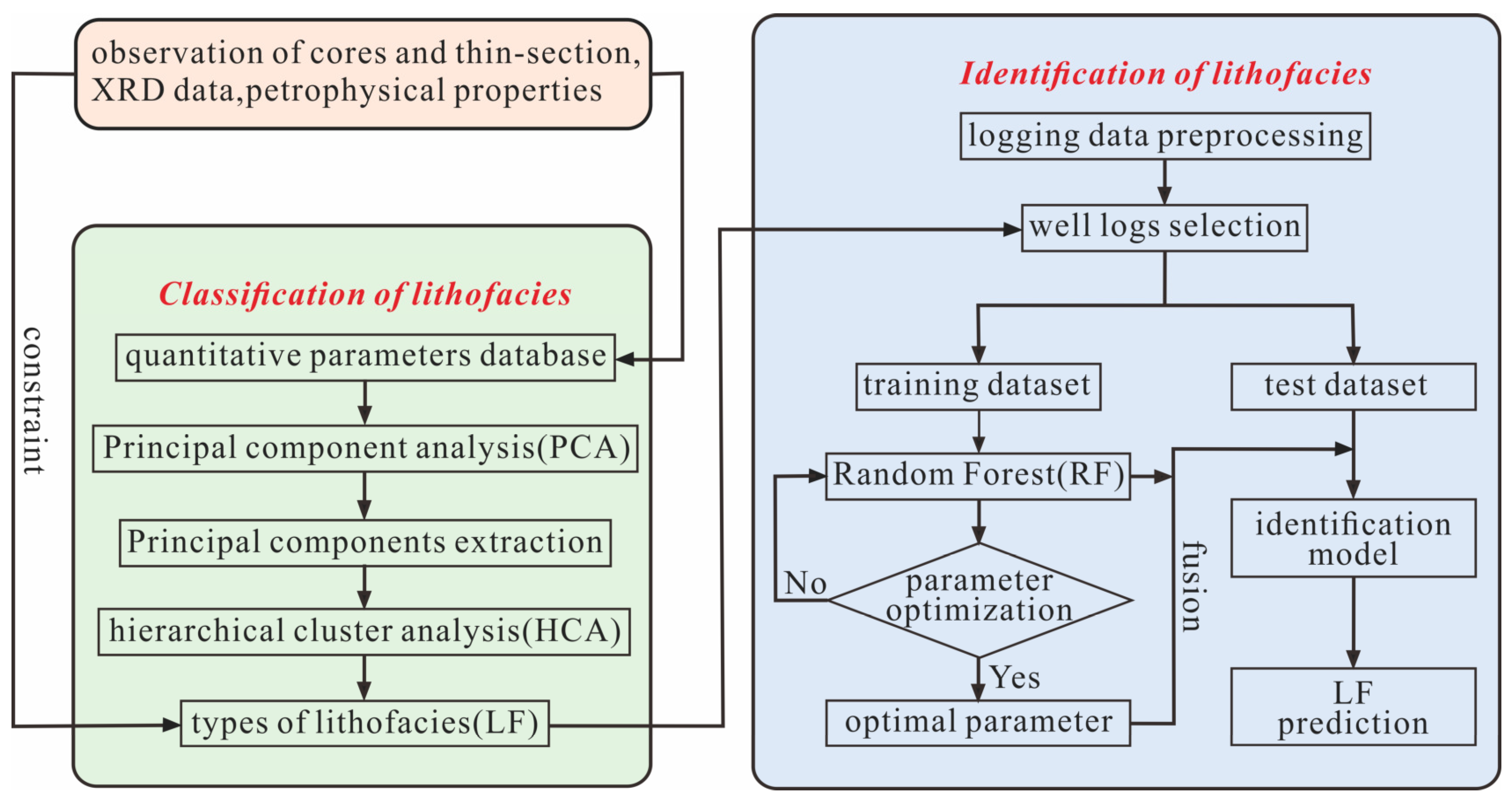
3.3. The Workflow of Lithofacies Prediction

The following is a brief description of the workflow of the lithofacies classification and logging identification (Figure 3). First, quantitative parameters were acquired based on XRD data, thin sections, and core observations. After standardization, 10 petrological and geochemical parameters were subjected to PCA, and PCs reflecting lithofacies information were obtained. Then, HCA was performed in accordance with the PCs of PCA to obtain the pedigree map. Lithofacies were classified, and the typical characteristics of different lithofacies were summarized. Subsequently, normalized logging data were selected by cross-plotting and matched with different lithofacies to establish the dataset used for lithofacies identification. The prediction model for mudrock lithofacies was established using GS–KCV–RF, and the identification accuracy was verified. The ranges for the parameters of the RF algorithm are determined by the GS and the optimal values of the parameters are determined with the KVC. Finally, the identification model was used to predict the lithofacies of the non-coring section.

4. Results

4.1. Quantitative Classification of Lithofacies

4.1.1. Principal Component Extraction

The basis for lithofacies classification of shale reservoirs usually includes mineralogical compositions, sedimentary textures and structures, TOC content, genesis, and petrophysical characteristics [8,11,12,31,58,59]. Petrological and geochemical data were fully mined for the quantitative classification of lithofacies, avoiding the uncertainty and subjectivity of artificial classification. A total of 10 parameters—mineralogical composition (the content of clay minerals, carbonate minerals, felsic terrigenous clastic minerals, and chlorite), reservoir parameters (porosity, permeability, oil saturation, and rock density), structure, and TOC content—were collected to characterize the lithofacies differences and characteristics of the third submember in the Bonan Sag. The structure of rocks includes massive structure and layered structure, which are assigned as 0 and 1, respectively. Different quantitative parameters indicate different information about lithofacies, and linear correlations exist between some parameters. The selection of excessive parameters leads to high dimensionality, which does not necessarily result in high recognition accuracy. High dimensionality reduces the running speed of an intelligent algorithm and makes it difficult to master the main information [24]. PCA was effectively used to reduce the dimensions of the parameters and transform them into a small set of uncorrelated variables.

To assess the appropriateness of the dataset for PCA, the Kaiser-Meyer-Olkin (KMO) test was conducted. This test evaluates the sampling adequacy by measuring the proportion of variance attributed to potential factors. A KMO value >0.5 is considered appropriate for PCA [60]. In this study, the KMO was 0.620 (>0.5), showing that PCA was feasible for the 10 parameters. After the data was processed by PCA, the correlation coefficient matrix of the lithofacies parameters after standardized processing was obtained. The Jacobian matrix was used to obtain the eigenvalues, unified eigenvectors, and variance contribution rate of the correlation coefficient matrix (

Table 2. The component score matrix, eigenvalues, variance contribution rate, and cumulative contribution rate after PCA processing.

PCs	Component Score Matrix										Eigenvalues	Variance Contribution Rate/%	Cumulative Contribution Rate/%
	Clay	Carb	Felsic	Chlorite	Porosity	Permeability	So	Density	Structure	TOC
PC1	0.194	−0.208	0.195	0.113	0.089	0.097	0.007	−0.196	−0.001	0.183	4.524	45.240	45.240
PC2	−0.027	0.035	0.023	0.335	−0.390	0.066	0.412	0.069	−0.055	0.097	2.161	21.610	66.850
PC3	−0.155	0.072	−0.004	−0.100	−0.075	0.518	−0.023	−0.020	0.691	0.055	1.259	12.590	79.440
PC4	0.291	−0.373	0.406	−0.102	−0.161	−0.656	0.190	0.350	0.606	−0.305	0.679	6.787	86.227
PC5	0.222	−0.338	0.318	−0.013	0.015	0.759	−0.014	0.554	−0.406	−0.767	0.525	5.254	91.482
PC6	0.647	0.036	−0.638	−0.609	0.334	0.135	1.040	−0.317	0.026	−0.204	0.392	3.919	95.400
PC7	0.045	0.214	−0.431	1.386	0.926	−0.130	0.038	−0.134	0.439	−0.724	0.266	2.657	98.057
PC8	−1.573	0.182	1.376	−0.417	0.905	−0.117	1.028	−0.624	−0.188	−0.426	0.141	1.414	99.472
PC9	−0.189	−0.023	−0.061	0.083	2.150	0.165	0.834	3.123	0.010	2.369	0.048	0.482	99.953
PC10	6.366	11.569	6.295	0.044	0.069	0.316	−0.354	0.569	0.025	0.069	0.005	0.047	100.000

Carb is short for carbonate minerals = calcite + dolomite; Felsic is short for felsic terrigenous clastic minerals = quartz + plagioclase + K-feldspar; So is short for oil saturation.

). The eigenvalues of PC1, PC2, PC3, and PC4 were all above 0.6, and their cumulative contribution rate was 86.227%, covering most of the original quantitative parameter information. Therefore, it was reasonable to select four PCs to replace the original ten parameters.

According to the eigenvector matrix, the PC1, PC2, PC3, and PC4 transformation equations for lithofacies classification were obtained as follows (Table 2):

PC1 = 0.194 clay − 0.208 carb + 0.195 felsic + 0.113 chlorite + 0.089 porosity+ 0.097 permeability + 0.007 So − 0.196 density − 0.001 structure + 0.183 TOC.

PC2 = −0.027 clay + 0.035 carb + 0.023 felsic + 0.335 chlorite − 0.390 porosity+ 0.066 permeability + 0.412 So + 0.069 density − 0.055 structure + 0.097 TOC.

PC3 = −0.155 clay + 0.072 carb − 0.004 felsic − 0.100 chlorite − 0.075 porosity+ 0.518 permeability − 0.023 So − 0.020 density + 0.691 structure + 0.055 TOC.

PC4 = 0.291 clay − 0.373 carb + 0.406 felsic − 0.102 chlorite − 0.161 porosity − 0.656 Permeability + 0.190 So + 0.350 density + 0.606 structure − 0.305 TOC.

4.1.2. Types of Lithofacies

Cluster analysis of the four PCs obtained by PCA was performed to achieve automatic quantitative classification of the lithofacies. In this study, the clustering of 85 samples from Well L69 in Bonan Sag was achieved through the calculation of the distance between the nuclear points of the two types. Theoretically, the smaller the centroid distance D, the more similar the data of the same type, resulting in an increased number of clusters. The relationship between different samples was illustrated by a hierarchical tree diagram, and a centroid distance of 10 was selected, which shows five different clusters (Figure 4). The classification was confirmed to be rational, with the first group consisting of 26 samples, the second group with 19 samples, the third group with 8 samples, the fourth group with 22 samples, and the fifth group with 10 samples. This confirmation was supported by observations of cores and thin sections (Figure 5 and Figure 6), as well as the statistical analysis of key reservoir parameters (Figure 7, Figure 8 and Figure 9).

LF1 was called massive argillaceous limestone lithofacies (MAL). The mineralogical composition revealed that carbonate minerals (47%–65%) accounted for a higher percentage compared to clay minerals (12%–22%). Felsic terrigenous clastic mineral content was 16%–29%, with an average of 20% (Figure 7). The TOC abundance is 1.6%–4.9% (Figure 8). The structure of the sample is predominantly massive, characterized by a few presences of discontinuous laminae and the absence of macro-bedding. The clay and cryptocrystalline calcites were evenly mixed (Figure 5a,b).

The overall structure of LF2 displayed layering, devoid of the occurrence of alternating dark and light laminae (Figure 5c), and was called laminated calcareous claystone lithofacies (LCC). The content of clay minerals (26%–48%, average 34%) was higher than that of carbonate minerals (12%–43%, average 28%) (Figure 7), and the TOC content was 2%–5.4% (Figure 8). The cryptocrystalline calcites were uniformly blended with the argillaceous matter. The distribution of calcites and plant fragments along the bedding was observed to lack a clear orientation, whereas quartz particles were not usually distributed along the layers and were not oriented in any direction (Figure 5d).

LF3 was called an intermittent lamellar argillaceous limestone lithofacies (ILAL) and was characterized by its gray color and developed lamination. The light laminae, mainly microcrystalline calcite, were interbedded with the dark laminae, which were predominantly calcareous argillaceous. The calcite laminae were mostly lenticular and intermittent, and the continuity of a single layer was poor (Figure 6a,b). Moreover, the light laminae, which ranged from 150 to 350 μm, were larger than the dark laminae, which ranged from 50 to 100 μm in thickness. The carbonate content of this lithofacies was 36%–69%, whereas the clay and felsic content was lower than the carbonate content, of which the clay mineral content was approximately 11%–27% (average 21%) and the average felsic content was 29% (Figure 7). Organic substances were enriched along the layers, with an M-TOC of 2.4%–13.0% (Figure 8).

LF4 was dark grey throughout and clearly presented light and dark continuous laminated structures (Figure 6c). Based on thin-section observations, the light laminae were mainly composed of lenticular and banded cryptocrystalline calcite, and dark laminae were composed of clay. The light laminae with clearer boundaries were slightly thicker than the dark laminae (Figure 6d). In this lithofacies, the carbonate mineral content showed a greater variation (56%–80%) distributed in parallel laminates with good continuity. The clay mineral content was 8%–19%, the felsic terrigenous clastic mineral content was 10%–20% (Figure 7), and the M-TOC was 3.6%–12.4% with an average of 6.8% (Figure 8). Thus, LF4 was described as a continuous lamellar argillaceous limestone lithofacies (CLAL).

The typical characteristics of LF5 include a brownish-grey color, dark clay laminae intercalated in the light calcite laminae, and easily identifiable lamina boundaries. White calcites with clear shapes were observed in the core samples, and the calcites were recrystallized and observed under a microscope (Figure 6e). The thickness of light laminae composed of microcrystalline and phanerocrystalline carbonate varies greatly, with a value of 100–800 μm (Figure 6f). The carbonate content of this lithofacies was the highest, ranging between 69–89%; the clay and felsic mineral contents were both less than 15% (Figure 7). The organic matter exhibited favorable stratification, with the TOC predominantly ranging from 6.5% and 14.0% (Figure 8). LF5 was termed as laminated mixed shale lithofacies (LMS).

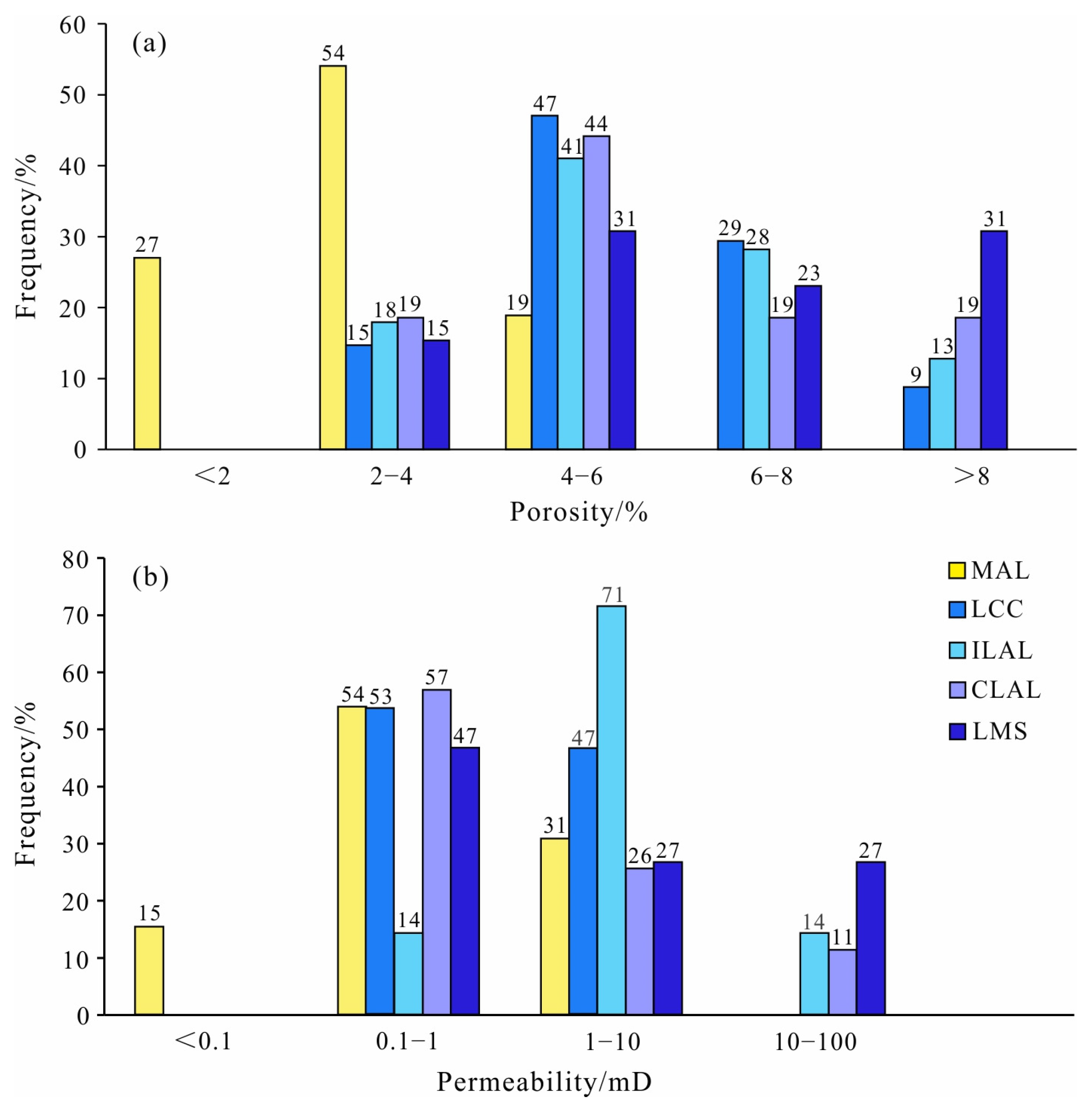
4.1.3. Petrophysical Characteristics of Different Lithofacies

The five types of lithofacies exhibited widely distributed porosities ranging from 1.2% to 10.4% (Figure 9a). The majority of MAL samples had porosities between 2% and 4%, with only a few falling below 2% or in the range of 4%–6%. No samples had porosities exceeding 6%. In contrast, 85% of LCC samples had porosities above 4%, primarily falling between 4% and 6%. The porosity distribution in ILAL exhibited two peaks: one at 4%–6% and another at 6%–8%. In CLAL, a peak at 4%–6% porosity was observed, accounting for 44% of the frequency, and 38% of the samples had porosities over 6%. The porosity range of LMS was from 3.3% to 11.0%, with most values exceeding 8%. Overall, LMS had the highest porosity, followed by CLAL, ILAL, and LCC, while MAL exhibited the lowest porosity.

Figure 9b shows that the LMS had the highest permeability, ranging from 10 to 100 mD, which accounted for 27% of the frequency. None of the samples had permeabilities below 0.1 mD. In ILAL, the main peak in permeability was observed at 1–10 mD, representing 71% of the frequency, whereas CLAL exhibited a permeability range from 0.12 mD to 100 mD, and LCC exhibited a permeability range from 0.5 mD to 8.2 mD. MAL has the lowest permeability range, with a peak at 0.1–1 mD and a few samples falling below 0.1 mD.

Based on the petrological information, TOC, and petrophysical characteristics, it was credible and reasonable to divide the five lithofacies of the third submember in the Bonan Sag. The dominant lithofacies conducive to shale oil enrichment were the LMS, CLAL, and ILAL.

4.2. Logging Identification for Lithofacies

Conventional well logs directly measure the petrophysical characteristics of subsurface rocks and are sensitive to variations in lithology, sedimentary texture, and structure, which are critical for building predictive models of lithofacies [22,61]. Logging identification models can be constructed using machine learning in the coring interval, and lithofacies can be predicted using well logs in the non-coring interval. The accuracy of the logging lithofacies identification depends on the availability of a sufficient number of samples. Accordingly, the data volume was expanded to 196 based on the results of the HCA and the quantitative statistics of the parameters.

Table 3. The distribution of different lithofacies samples in the dataset.

Lithofacies Type	Sample Size	Proportion
massive argillaceous limestone lithofacies (MAL)	44	22.45%
laminated calcareous claystone lithofacies (LCC)	43	21.94%
intermittent lamellar argillaceous limestone lithofacies (ILAL)	25	12.76%
continuous lamellar argillaceous limestone lithofacies (CLAL)	51	26.02%
laminated mixed shale lithofacies (LMS)	33	16.84%
total	196	100%

shows the distribution of different lithofacies. The database was randomly divided into training and test datasets according to 7:3.

4.2.1. Logging Parameters Selection

Well logs selection plays an important role in the logging identification of lithofacies. The logging parameters must be sensitive to at least one of the lithofacies, which is the most important factor in ensuring the accuracy of the lithofacies identification. In addition, the number of logging parameters should be appropriate, as this can affect the accuracy and training time of the prediction model.

The cross-plot of the well logs of different lithofacies indicates that: (1) GR, AC, and CNL can effectively distinguish LCC, CLAL, and LMS with varying clay mineral contents. (2) AC and LLD were sensitive to the four lithofacies, except for ILAL. (3) DEN and SP could identify MAL, CLAL, and LMS with different textures. (4) It was difficult for LLS and CAL to effectively distinguish different lithofacies because most of the points were mixed in the cross-plot (Figure 10). Therefore, six logging parameters were selected for lithofacies identification based on a full consideration of the quality and resolution ability: GR, AC, CNL, LLD, DEN, and SP.

4.2.2. Logging Response and Lithofacies Comparison

MAL lithofacies are mostly characterized by medium radioactivity, low porosity, and permeability. Therefore, it has medium to high GR (44–62 API) and DEN (2.49–2.56 g/cm³) values, high SP (32–40 mV) and CNL (18%–27%), relatively low to medium AC (69–82 μs/ft), and low resistivity (10–82 Ω·m) values. The LCC lithofacies had the highest GR (>70 API), medium SP (29–32 mV), high CNL (24%–35%), low to medium DEN values (2.46–2.50 g/cm³), medium to high AC values (85–106 μs/ft), and medium LLD (105–133 Ω·m). The ILAL lithofacies had low to medium GR and DEN, low SP, low to medium CNL, and high AC and LLD values, with low porosity and high permeability. The CLAL lithofacies had medium to high GR, high SP, high DEN (>2.61 g/cm³), low CNL and AC, and low to medium LLD values. The LMS lithofacies had the highest carbonate content (average 80%), and carbonate minerals displayed attributes of low radioactivity and hydrogen index, high density, and limited electrical conductivity. Therefore, the LMS lithofacies had low to medium GR and CNL, low SP and DEN, high AC, and medium LLD (

Table 4. Conventional well logs’ response value of the five lithofacies.

Lithofacies	GR (API)	SP (mV)	CNL (%)	DEN (g/cm3)	AC (μs/ft)	LLD (Ω·m)
MAL	44–62 51	32–40 36	18–27 23	2.49–2.56 2.52	69–92 85	10–82 32
LCC	70–92 86	29–32 30	18–25 22	2.48–2.54 2.50	76–93 86	105–133 119
ILAL	58–74 63	22–29 26	16–30 20	2.43–2.56 2.50	74–105 93	205–483 334
CLAL	40–57 48	33–40 38	7–15 12	2.56–2.66 2.61	62–83 71	11–96 43
LMS	37–56 47	20–30 26	19–24 22	2.35–2.48 2.45	75–102 91	82–107 106

$\frac{\mathrm{M}\mathrm{i}\mathrm{n}-\mathrm{M}\mathrm{a}\mathrm{x}}{\mathrm{A}\mathrm{v}\mathrm{e}}.$

).

The values of the same logging parameters for these five lithofacies overlapped significantly. However, certain trends were still discernible when comparing the logging values of the various lithofacies (Figure 11):

(1)

The GR values of the lithofacies can be divided into three levels. The LCC lithofacies exhibited the highest values. The GR values of the CLAL lithofacies were similar to the MAL lithofacies. The ILAL and LMS lithofacies had the lowest values.

(2)

The SP values of the MAL and CLAL lithofacies were the highest, followed by those of the LCC lithofacies. The SP values of the ILAL and LMS lithofacies are the lowest.

(3)

The CNL values of the five lithofacies had little difference, but the values of the CLAL lithofacies were slightly lower than those of the other four lithofacies.

(4)

The DEN values were the highest for CLAL lithofacies and lowest for LMS lithofacies. The MAL, LCC, and ILAL lithofacies, in second place, had a similar DEN value.

(5)

The AC values of the ILAL and LMS lithofacies were the highest with the development of a laminar structure, followed by the MAL and LCC lithofacies, whereas the CLAL lithofacies were the lowest.

(6)

The LLD values of the ILAL lithofacies were the highest because of the high TOC content and poor electrical conductivity of the kerogen, whereas those of the LCC and LMS lithofacies were lower. The MAL and CLAL lithofacies had the lowest LLD values.

4.2.3. GS–KCV–RF for Lithofacies Identification

Many parameters have a great influence on the performance of the lithofacies identification model based on RF: (1) Too many decision trees make the model overfit and too few make the model underfit. (2) The maximum tree depth is employed to manage the complexity of the model. Too large or too small a depth will lead to overfitting and reduce the accuracy of the model. (3) The number of features during tree splitting determines the correlation of trees, and the model is accurate with a low correlation of trees. Combine GS and KVC to select the best parameters to improve the accuracy of the RF model. Due to the small number of samples, four-fold cross-verification is used. Due to the small sample size, K-fold cross-validation divides the original data into four groups (K = 4). Take one subset as the primary validation set without repetition, and the other three subsets as the new training set, and cycle four times. The cross-validation score of RF is obtained from the average of the four model validation scores. The GS is an exhaustive search method. Within the preset parameter range, the adjusted parameters are used in random forest training to find the parameter combination with the maximum cross-validation score of the model, which can effectively avoid the overfitting or underfitting of the model.

Table 5. Parameter tuning for random forest.

Parameters	Search Range	Step Size	Optimal Value
the number of decision trees	10~200	10	50
the maximum tree depth	1~15	1	10
the number of features when the tree splits	1~6	1	3

shows the range of parameters and the optimal values of them for parameter tuning. The RF model is trained on MATLAB with a training dataset, and the importance scores of six logging parameters are given (Figure 12). CNL was the most important factor for the identification of different lithofacies, followed by SP, AC, DEN, and LNLLD, while GR exhibited the lowest influence.

4.2.4. Verification of Identification Accuracy

In this study, accuracy, precision, recall, and F1-score are used to evaluate the performance of the classification model. Accuracy represents the ratio of correctly identified results to the total number of samples examined. Precision signifies the proportion of correctly identified true positives among the predicted positive results. Recall is the ratio of the predicted positive to the total positive samples. F1-score is calculated as the harmonic mean of precision and recall, which is valuable for handling datasets with numerous categories. The performance metrics are defined as the following equations:

$$\mathrm{A}\mathrm{c}\mathrm{c}\mathrm{u}\mathrm{r}\mathrm{a}\mathrm{c}\mathrm{y}=\frac{\mathrm{T}\mathrm{P}+\mathrm{T}\mathrm{N}}{TP+TN+FP+FN}\times 100\%$$

(2)

$$\mathrm{P}\mathrm{r}\mathrm{e}\mathrm{c}\mathrm{i}\mathrm{s}\mathrm{i}\mathrm{o}\mathrm{n}=\frac{\mathrm{T}\mathrm{P}}{TP+ FP }\times 100\%$$

(3)

$$\mathrm{R}\mathrm{e}\mathrm{c}\mathrm{a}\mathrm{l}\mathrm{l}=\frac{\mathrm{T}\mathrm{P}}{TP+ FN }\times 100\%$$

(4)

$$\mathrm{F}1-\mathrm{s}\mathrm{c}\mathrm{o}\mathrm{r}\mathrm{e}=\frac{2\times \mathrm{P}\mathrm{r}\mathrm{e}\mathrm{c}\mathrm{i}\mathrm{s}\mathrm{i}\mathrm{o}\mathrm{n}\times \mathrm{R}\mathrm{e}\mathrm{c}\mathrm{a}\mathrm{l}\mathrm{l}}{Precision+Recall }\times 100\%$$

(5)

TP, TN, FP, and FN stand for true positive, true negative, false positive, and false negative, respectively. Precision, recall, and F1-score range from 0 to 100%, with 1 indicating the best model classification performance.

The validation methods included internal, external, and holdout prediction verification. First, in the internal verification, the trained random forest model is used to identify the training dataset individually, and consistency between the predicted lithofacies classification of each sample and the core definition lithofacies was observed. The training dataset performed well with an accuracy of 100%, and precision, recall, and Fl- scores were all 100% (

Table 6. Accuracy, precision, recall, and F1-score for lithofacies identification over random forest.

Lithofacies	Training Datasets				Test Datasets
	Accuracy	Precision	Recall	F1-Score	Accuracy	Precision	Recall	F1-Score
MAL	100.0%	100.0%	100.0%	100.0%	98.3%	100.0%	87.5%	93.3%
LCC	100.0%	100.0%	100.0%	100.0%	96.6%	90.9%	90.9%	90.9%
ILAL	100.0%	100.0%	100.0%	100.0%	98.3%	83.3%	100.0%	90.9%
CLAL	100.0%	100.0%	100.0%	100.0%	100.0%	100.0%	100.0%	100.0%
LMS	100.0%	100.0%	100.0%	100.0%	96.6%	91.7%	91.7%	91.7%
Average	100.0%	100.0%	100.0%	100.0%	97.9%	93.2%	94.0%	93.4%

). External verification can be used to test the practical effectiveness of the model. The identification results were obtained by substituting the testing dataset into the RF model (Figure 13), and the overall accuracy was 97.9%. CLAL yielded the highest accuracy among five lithofacies, with an F1-score of 1. ILAL had the worst precisions, which were often mistakenly predicted as LMS. The F1-score of all the other lithofacies were above 90% (Table 6). Finally, the L69 well with enough geological data was used as a test set to study the consistency of lithofacies prediction using the RF method. As shown in Figure 14, the lithofacies predicted by the RF model coincided with the lithofacies identified through the thin-section observations and XRD analysis of the core samples. The accuracy of holdout prediction validation reached an average of 93.2%. The precision of lithofacies identification using the three verification methods showed a good recognition effect, with an accuracy greater than 93%.

5. Discussion

5.1. Performances and Improvements of Machine-Learning Models

In this study, a complete technical workflow for mudrock lithofacies classification and prediction utilizing machine learning was proposed. PCA and HCA were used to realize the quantitative classification of lithofacies, which can automatically classify according to the similarity of petrological and petrophysical properties without prior classification. Then, we take lithofacies types determined by HCA as the output of the train dataset and use random forest (RF) to construct logging identification models with high recognition accuracy. HCA offers the benefit of utilizing the internal data relationship without the disturbance of human factors to determine lithofacies, resulting in a significantly reduced time while ensuring the precision of lithofacies classification. The use of PCA and HCA improves the efficiency and reliability of lithofacies classification. RF is applied for the lithofacies prediction based on well logs in a classification course. RF, in comparison to other machine-learning methods, offers simplicity in usage and the capability to handle high-dimensional input features. Estimating the importance of features during the training course can obtain a quantitative index in selecting features, thereby decreasing training costs. In particular, the RF model excels in generalization, enabling efficient utilization across diverse formations or basins. To optimize the RF performance, various hyperparameters need to be selected, including the number of decision trees and features [62]. In this research, we employed grid search combined with K-fold cross-validation to determine the optimal parameters to improve the accuracy of RF model. The RF model had an overall accuracy of 93.2%, while He et al. [22] used the same dataset to identify shale lithofacies with an accuracy of 80.9%. The RF model can accurately predict lithofacies, and the performance is significantly improved compared to other studies using the same dataset.

Unlike prior research that focused on overall accuracy, this study conducted a comprehensive evaluation of each lithofacies class, considering multiple metrics such as accuracy, precision, recall, and F1-score. CLAL is completely correctly identified with all performance metrics achieving 100%. ILAL has accuracy, precision, recall, and F1-score of about 98.3%, 83.3%, 100.0%%, and 90.9%, respectively, and LMS has results of about 96.6%, 91.7%, 91.7%, and 91.7%, respectively, which is inferior to the other lithofacies. The relatively lower accuracy in predicting ILAL and LMS may arise from their less significant features compared with CLAL, MAL, and LCC and low distribution in the whole lithofacies.

Though the complete technical workflow for machine learning show advantages in mudrock lithofacies classification and prediction with a high accuracy and efficiency, improvements are still necessary. Within this research, an imbalanced lithofacies distribution is observed, and the ILAL, occupying only 12.76% of the entire dataset, exhibit asignificantly lower distribution compared to other lithofacies (Table 3). The RF model assigns greater weight to the lithofacies that are more enriched, resulting in enhanced performance for these lithofacies but leading to a decrease in the performance for ILAL. ILAL is often identified as LMS (Figure 13), suggesting that the existing features are insufficient for effectively distinguishing ILAL lithofacies from others. Additionally, the present RF model exhibits excessive sensitivity to alterations in well log data, resulting in the potential overexplanation of lithofacies. The machine-learning model currently in use inadvertently captures minor fluctuations in well log values caused by reservoir heterogeneities, which should be disregarded as they do not reflect actual lithofacies changes. Further improvements can be made from three aspects. A balanced lithofacies dataset, created by data resampling techniques (combining SMOTE and NCR methods), is needed to address the influence of imbalanced original datasets on lithofacies identification [63]. Additionally, domain knowledge, such as lithological and lithofacies stacking patterns, is necessary to be incorporated into RF models for the extraction of crucial features to enhance lithofacies identifications [64]. To mitigate the excessive sensitivity of RF, future efforts can involve training the dataset with appropriate encoders and decoders for the extraction of low-frequency and high-frequency data, and employing the mechanism of attention to effectively reduce the noise present in loggings [65,66].

5.2. Applications of Machine-Learning Models

The logging identification model was applied to predict the lithofacies of the 1982 m formation in six wells (L813, L69, Y177, Y289, Y283, and Y288) to systematically analyze the distribution characteristics of the third submember lithofacies in the Bonan Sag. Sequence stratigraphy plays a significant role in shale oil exploration as it allows for the analysis and understanding of the spatial and temporal distributions of sedimentary systems [67]. Previous studies have shown that the third submember is a complete third-order sequence, reflecting a complete regional rise and fall at lake level. However, due to the lack of a lacustrine slope break zone, the sequences of the third submember in Bonan Sag were subdivided into the transgressive systems tract (TST), the early highstand systems tract (EHST), and the late highstand systems tract (LHST) [68,69]. Under the sequence stratigraphic framework, a cross-well profile from the Southern Gentle Slope Zone to Boshen4 Step-Fault Zone, Bonan Deep Sag Zone, and Northern Steep Slope Zone was plotted based on the results of the single-well lithofacies division (Figure 15). The lithofacies of the TST were dominated by LMS and CLAL, and the thicknesses of the deposits were relatively uniform. A continuous thick-layered CLAL with stable distribution was observed, and the LMS thickened first, and then thinned from south to north, transitioning to the LCC in the Northern Steep Slope Zone. The thickness of the EHST deposits increased gradually from south to north, and there was a large horizontal difference in lithofacies, which was composed of LMS, LCC, and ILAL. In the Southern Gentle Slope Zone, the LCC was mainly developed and sandwiched between thin lamellar LMS. To the north of well Y177, the lithofacies were mainly ILAL interbedded with LMS and LCC. The LHST was characterized by a thickened MAL from south to north and a stable distribution of thin-layered ILAL. Simultaneously, the LMS decreased from south to north, and the LCC developed only in the Northern Steep Slope Zone. As the petrophysical characteristics in Section 4.2 showed that the dominant lithofacies conducive to shale oil enrichment were LMS, CLAL, and ILAL, the horizontal distribution of lithofacies indicated that the favorable target areas of shale oil in the Bonan Sag were mainly concentrated in the Boshen4 Step-Fault Zone and Bonan Deep Sag Zone.

During the deposition of the third submember in the Bonan Sag, the lake was generally alkaline and highly saline, and the climate changed from relatively arid to humid, indicating a typical deep to intermediate-depth environment [70,71,72]. The LMS had high levels of clay minerals in the shale, usually indicating a deep water and quiet sedimentary environment [73,74,75]. The LCC also occurred in a deep lake environment, but at slightly shallower depths and under higher hydrodynamic conditions than the LMS [76,77]. The CLAL and ILAL were formed in relative shallow, stratified, and highly productive conditions [72,74]. The MAL developed in a shallowing water body that was less stratified, with high productivity [71,72]. The lithofacies characteristics revealed obvious changes in the progression of the deposition of the third submember, indicating a rising lake level, and then a fall from the TST to LHST, which corresponded well with the previous systems tract division of Liu et al. [68].

6. Conclusions

In this study, a complete workflow for the automatic classification and logging prediction of mudrock lithofacies was established. This workflow integrated three machine-learning algorithms (PCA, HCA, and optimized RF) to completely mine the data and provided a reference for the quantitative classification and identification of lithofacies in other areas. The following findings can be summarized based on the results presented above:

• Instead of previous manual classification, PCA and HCA automatically classify mudrock lithofacies of the third submember reservoir in the Bonan Sag into five types: MAL, LCC, ILAL, CLAL, and LMS. The lithofacies classification of PCA and HCA, according to the similarity of the samples’ known petrological and petrophysical properties, can streamline decision-making processes and increase efficiency in lithofacies classification.
• The RF model, optimized by GS and KCV, effectively predicts mudrock lithofacies from conventional logging data in non-cored intervals. The values of accuracy, precision, recall, and F1-score is 97.7%, 93.2%, 94.0%, and 93.4%, respectively.
• The horizontal distribution of lithofacies that was predicted by machine-learning models indicated that the favorable areas for petroleum exploration in the Bonan Sag were the Boshen4 Step-Fault Zone and Bonan Deep Sag Zone.

References

1. Hickey, J.J.; Henk, B. Lithofacies Summary of the Mississippian Barnett Shale, Mitchell 2 T.P. Sims Well, Wise County, Texas. AAPG Bull. 2007, 91, 437–443. [Google Scholar] [CrossRef]
2. Ou, C.; Li, C.; Rui, Z.; Ma, Q. Lithofacies Distribution and Gas-Controlling Characteristics of the Wufeng–Longmaxi Black Shales in the Southeastern Region of the Sichuan Basin, China. J. Pet. Sci. Eng. 2018, 165, 269–283. [Google Scholar] [CrossRef]
3. Jamil, M.; Siddiqui, N.A.; Usman, M.; Wahid, A.; Umar, M.; Ahmed, N.; Haq, I.U.; El-Ghali, M.A.K.; Imran, Q.S.; Rahman, A.H.A.; et al. Facies Analysis and Distribution of Late Palaeogene Deep-water Massive Sandstones in Submarine-fan Lobes, NW Borneo. Geol. J. 2022, 57, 4489–4507. [Google Scholar] [CrossRef]
4. Jamil, M.; Siddiqui, N.A.; Ahmed, N.; Usman, M.; Umar, M.; Rahim, H.U.; Imran, Q.S. Facies Analysis and Sedimentary Architecture of Hybrid Event Beds in Submarine Lobes: Insights from the Crocker Fan, NW Borneo, Malaysia. JMSE 2021, 9, 1133. [Google Scholar] [CrossRef]
5. Sayed, M.A.; Al-Muntasheri, G.A.; Liang, F. Development of Shale Reservoirs: Knowledge Gained from Developments in North America. J. Pet. Sci. Eng. 2017, 157, 164–186. [Google Scholar] [CrossRef]
6. Zhu, H.; Kong, X.; Long, H.; Huai, Y. Duvernay Shale Lithofacies Distribution Analysis in the West Canadian Sedimentary Basin. IOP Conf. Ser. Earth Environ. Sci. 2018, 121, 052007. [Google Scholar] [CrossRef]
7. Abouelresh, M.O.; Slatt, R.M. Lithofacies and Sequence Stratigraphy of the Barnett Shale in East-Central Fort Worth Basin, Texas. AAPG Bull. 2012, 96, 1–22. [Google Scholar] [CrossRef]
8. Bai, C.; Yu, B.; Han, S.; Shen, Z. Characterization of Lithofacies in Shale Oil Reservoirs of a Lacustrine Basin in Eastern China: Implications for Oil Accumulation. J. Pet. Sci. Eng. 2020, 195, 107907. [Google Scholar] [CrossRef]
9. Chen, X.; Wang, C.; Kuhnt, W.; Holbourn, A.; Huang, Y.; Ma, C. Lithofacies, Microfacies and Depositional Environments of Upper Cretaceous Oceanic Red Beds (Chuangde Formation) in Southern Tibet. Sediment. Geol. 2011, 235, 100–110. [Google Scholar] [CrossRef]
10. Dong, T.; Harris, N.B.; Ayranci, K.; Twemlow, C.E.; Nassichuk, B.R. Porosity Characteristics of the Devonian Horn River Shale, Canada: Insights from Lithofacies Classification and Shale Composition. Int. J. Coal Geol. 2015, 141–142, 74–90. [Google Scholar] [CrossRef]
11. Loucks, R.G.; Ruppel, S.C. Mississippian Barnett Shale: Lithofacies and Depositional Setting of a Deep-Water Shale-Gas Succession in the Fort Worth Basin, Texas. AAPG Bull. 2007, 91, 579–601. [Google Scholar] [CrossRef]
12. Wang, G.; Cheng, G.; Carr, T.R. The Application of Improved NeuroEvolution of Augmenting Topologies Neural Network in Marcellus Shale Lithofacies Prediction. Comput. Geosci. 2013, 54, 50–65. [Google Scholar] [CrossRef]
13. Wang, P.; Jiang, Z.; Yin, L.; Chen, L.; Li, Z.; Zhang, C.; Li, T.; Huang, P. Lithofacies Classification and Its Effect on Pore Structure of the Cambrian Marine Shale in the Upper Yangtze Platform, South China: Evidence from FE-SEM and Gas Adsorption Analysis. J. Pet. Sci. Eng. 2017, 156, 307–321. [Google Scholar] [CrossRef]
14. Xue, C.; Wu, J.; Qiu, L.; Zhong, J.; Zhang, S.; Zhang, B.; Wu, X.; Hao, B. Lithofacies Classification and Its Controls on the Pore Structure Distribution in Permian Transitional Shale in the Northeastern Ordos Basin, China. J. Pet. Sci. Eng. 2020, 195, 107657. [Google Scholar] [CrossRef]
15. Zhao, C.; Jiang, Y.; Wang, L. Data-Driven Diagenetic Facies Classification and Well-Logging Identification Based on Machine Learning Methods: A Case Study on Xujiahe Tight Sandstone in Sichuan Basin. J. Pet. Sci. Eng. 2022, 217, 110798. [Google Scholar] [CrossRef]
16. Kadkhodaie, A.; Rezaee, R. Intelligent Sequence Stratigraphy through a Wavelet-Based Decomposition of Well Log Data. J. Nat. Gas Sci. Eng. 2017, 40, 38–50. [Google Scholar] [CrossRef]
17. Li, Z.; Zhang, L.; Yuan, W.; Chen, X.; Zhang, L.; Li, M. Logging Identification for Diagenetic Facies of Tight Sandstone Reservoirs: A Case Study in the Lower Jurassic Ahe Formation, Kuqa Depression of Tarim Basin. Mar. Pet. Geol. 2022, 139, 105601. [Google Scholar] [CrossRef]
18. Sun, Y.; Chen, J.; Yan, P.; Zhong, J.; Sun, Y.; Jin, X. Lithology Identification of Uranium-Bearing Sand Bodies Using Logging Data Based on a BP Neural Network. Minerals 2022, 12, 546. [Google Scholar] [CrossRef]
19. Wei, Z.; Hu, H.; Zhou, H.; Lau, A. Characterizing Rock Facies Using Machine Learning Algorithm Based on a Convolutional Neural Network and Data Padding Strategy. Pure Appl. Geophys. 2019, 176, 3593–3605. [Google Scholar] [CrossRef]
20. Antariksa, G.; Muammar, R.; Lee, J. Performance Evaluation of Machine Learning-Based Classification with Rock-Physics Analysis of Geological Lithofacies in Tarakan Basin, Indonesia. J. Pet. Sci. Eng. 2022, 208, 109250. [Google Scholar] [CrossRef]
21. Dong, S.-Q.; Zhong, Z.-H.; Cui, X.-H.; Zeng, L.-B.; Yang, X.; Liu, J.-J.; Sun, Y.-M.; Hao, J.-R. A Deep Kernel Method for Lithofacies Identification Using Conventional Well Logs. Pet. Sci. 2023, 20, 1411–1428. [Google Scholar] [CrossRef]
22. He, J.; Ding, W.; Jiang, Z.; Li, A.; Wang, R.; Sun, Y. Logging Identification and Characteristic Analysis of the Lacustrine Organic-Rich Shale Lithofacies: A Case Study from the Es 3 L Shale in the Jiyang Depression, Bohai Bay Basin, Eastern China. J. Pet. Sci. Eng. 2016, 145, 238–255. [Google Scholar] [CrossRef]
23. Dubois, M.K.; Bohling, G.C.; Chakrabarti, S. Comparison of Four Approaches to a Rock Facies Classification Problem. Comput. Geosci. 2007, 33, 599–617. [Google Scholar] [CrossRef]
24. Zheng, W.; Tian, F.; Di, Q.; Xin, W.; Cheng, F.; Shan, X. Electrofacies Classification of Deeply Buried Carbonate Strata Using Machine Learning Methods: A Case Study on Ordovician Paleokarst Reservoirs in Tarim Basin. Mar. Pet. Geol. 2021, 123, 104720. [Google Scholar] [CrossRef]
25. Corina, A.N.; Hovda, S. Automatic Lithology Prediction from Well Logging Using Kernel Density Estimation. J. Pet. Sci. Eng. 2018, 170, 664–674. [Google Scholar] [CrossRef]
26. Moja, S.S.; Asfaw, Z.G.; Omre, H. Bayesian Inversion in Hidden Markov Models with Varying Marginal Proportions. Math. Geosci. 2019, 51, 463–484. [Google Scholar] [CrossRef]
27. Bressan, T.S.; Kehl de Souza, M.; Girelli, T.J.; Junior, F.C. Evaluation of Machine Learning Methods for Lithology Classification Using Geophysical Data. Comput. Geosci. 2020, 139, 104475. [Google Scholar] [CrossRef]
28. Xie, Y.; Zhu, C.; Zhou, W.; Li, Z.; Liu, X.; Tu, M. Evaluation of Machine Learning Methods for Formation Lithology Identification: A Comparison of Tuning Processes and Model Performances. J. Pet. Sci. Eng. 2018, 160, 182–193. [Google Scholar] [CrossRef]
29. Hall, B. Facies Classification Using Machine Learning. Lead. Edge 2016, 35, 906–909. [Google Scholar] [CrossRef]
30. Liu, B.; Zhao, X.; Fu, X.; Yuan, B.; Bai, L.; Zhang, Y.; Ostadhassan, M. Petrophysical Characteristics and Log Identification of Lacustrine Shale Lithofacies: A Case Study of the First Member of Qingshankou Formation in the Songliao Basin, Northeast China. Interpretation 2020, 8, SL45–SL57. [Google Scholar] [CrossRef]
31. Wang, G.; Carr, T.R.; Ju, Y.; Li, C. Identifying Organic-Rich Marcellus Shale Lithofacies by Support Vector Machine Classifier in the Appalachian Basin. Comput. Geosci. 2014, 64, 52–60. [Google Scholar] [CrossRef]
32. Al-Mudhafar, W.J. Integrating Well Log Interpretations for Lithofacies Classification and Permeability Modeling through Advanced Machine Learning Algorithms. J. Pet. Explor Prod Technol 2017, 7, 1023–1033. [Google Scholar] [CrossRef]
33. Bhatt, A.; Helle, H.B. Determination of Facies from Well Logs Using Modular Neural Networks. Pet. Geosci. 2002, 8, 217–228. [Google Scholar] [CrossRef]
34. He, J.; La Croix, A.D.; Wang, J.; Ding, W.; Underschultz, J.R. Using Neural Networks and the Markov Chain Approach for Facies Analysis and Prediction from Well Logs in the Precipice Sandstone and Evergreen Formation, Surat Basin, Australia. Mar. Pet. Geol. 2019, 101, 410–427. [Google Scholar] [CrossRef]
35. Dev, V.A.; Eden, M.R. Formation Lithology Classification Using Scalable Gradient Boosted Decision Trees. Comput. Chem. Eng. 2019, 128, 392–404. [Google Scholar] [CrossRef]
36. Nguyen, H.; Savary-Sismondini, B.; Patacz, V.; Jenssen, A.; Kifle, R.; Bertrand, A. Application of Random Forest Algorithm to Predict Lithofacies from Well and Seismic Data in Balder Field, Norwegian North Sea. AAPG Bull. 2022, 106, 2239–2257. [Google Scholar] [CrossRef]
37. Tewari, S.; Dwivedi, U.D. Ensemble-Based Big Data Analytics of Lithofacies for Automatic Development of Petroleum Reservoirs. Comput. Ind. Eng. 2019, 128, 937–947. [Google Scholar] [CrossRef]
38. Valentín, M.B.; Bom, C.R.; Coelho, J.M.; Correia, M.D.; de Albuquerque, M.P.; de Albuquerque, M.P.; Faria, E.L. A Deep Residual Convolutional Neural Network for Automatic Lithological Facies Identification in Brazilian Pre-Salt Oilfield Wellbore Image Logs. J. Pet. Sci. Eng. 2019, 179, 474–503. [Google Scholar] [CrossRef]
39. Bhattacharya, S.; Carr, T.R.; Pal, M. Comparison of Supervised and Unsupervised Approaches for Mudstone Lithofacies Classification: Case Studies from the Bakken and Mahantango-Marcellus Shale, USA. J. Nat. Gas Sci. Eng. 2016, 33, 1119–1133. [Google Scholar] [CrossRef]
40. Wang, G.; Carr, T.R. Marcellus Shale Lithofacies Prediction by Multiclass Neural Network Classification in the Appalachian Basin. Math. Geosci. 2012, 44, 975–1004. [Google Scholar] [CrossRef]
41. Liu, H.; Jiang, Y.; Song, G.; Gu, G.; Hao, L.; Feng, Y. Overpressure Characteristics and Effects on Hydrocarbon Distribution in the Bonan Sag, Bohai Bay Basin, China. J. Pet. Sci. Eng. 2017, 149, 811–821. [Google Scholar] [CrossRef]
42. Han, S.; Yu, B.; Ruan, Z.; Bai, C.; Shen, Z.; Löhr, S.C. Diagenesis and Fluid Evolution in the Third Member of the Eocene Shahejie Formation, Bonan Sag, Bohai Bay Basin, China. Mar. Pet. Geol. 2021, 128, 105003. [Google Scholar] [CrossRef]
43. Wang, M.; Wilkins, R.W.T.; Song, G.; Zhang, L.; Xu, X.; Li, Z.; Chen, G. Geochemical and Geological Characteristics of the Es3L Lacustrine Shale in the Bonan Sag, Bohai Bay Basin, China. Int. J. Coal Geol. 2015, 138, 16–29. [Google Scholar] [CrossRef]
44. An, T.; Yu, B.; Wang, Y.; Ruan, Z.; Meng, W.; Feng, Y. Water-Rock Interactions and Origin of Formation Water in the Bohai Bay Basin: A Case Study of the Cenozoic Formation in Bonan Sag. Interpretation 2021, 9, T475–T493. [Google Scholar] [CrossRef]
45. Jiu, K.; Ding, W.; Huang, W.; Zhang, Y.; Zhao, S.; Hu, L. Fractures of Lacustrine Shale Reservoirs, the Zhanhua Depression in the Bohai Bay Basin, Eastern China. Mar. Pet. Geol. 2013, 48, 113–123. [Google Scholar] [CrossRef]
46. Adler, N.; Golany, B. Including Principal Component Weights to Improve Discrimination in Data Envelopment Analysis. J. Oper. Res. Soc. 2002, 53, 985–991. [Google Scholar] [CrossRef]
47. Ma, Y.Z. Lithofacies Clustering Using Principal Component Analysis and Neural Network: Applications to Wireline Logs. Math. Geosci. 2011, 43, 401–419. [Google Scholar] [CrossRef]
48. Alzubi, J.; Nayyar, A.; Kumar, A. Machine Learning from Theory to Algorithms: An Overview. J. Phys. Conf. Ser. 2018, 1142, 012012. [Google Scholar] [CrossRef]
49. Petroni, A.; Braglia, M. Vendor Selection Using Principal Component Analysis. J. Supply Chain Manag. 2000, 36, 63–69. [Google Scholar] [CrossRef]
50. Ghosh, S.; Chatterjee, R.; Shanker, P. Estimation of Ash, Moisture Content and Detection of Coal Lithofacies from Well Logs Using Regression and Artificial Neural Network Modelling. Fuel 2016, 177, 279–287. [Google Scholar] [CrossRef]
51. Sfidari, E.; Kadkhodaie-Ilkhchi, A.; Najjari, S. Comparison of Intelligent and Statistical Clustering Approaches to Predicting Total Organic Carbon Using Intelligent Systems. J. Pet. Sci. Eng. 2012, 86–87, 190–205. [Google Scholar] [CrossRef]
52. Bubnova, A.; Ors, F.; Rivoirard, J.; Cojan, I.; Romary, T. Automatic Determination of Sedimentary Units from Well Data. Math. Geosci. 2020, 52, 213–231. [Google Scholar] [CrossRef]
53. Rahimi, M.; Riahi, M.A. Reservoir Facies Classification Based on Random Forest and Geostatistics Methods in an Offshore Oilfield. J. Appl. Geophys. 2022, 201, 104640. [Google Scholar] [CrossRef]
54. Wang, Z.; Cai, Y.; Liu, D.; Qiu, F.; Sun, F.; Zhou, Y. Intelligent Classification of Coal Structure Using Multinomial Logistic Regression, Random Forest and Fully Connected Neural Network with Multisource Geophysical Logging Data. Int. J. Coal Geol. 2023, 268, 104208. [Google Scholar] [CrossRef]
55. Jiang, F.; Huo, L.; Chen, D.; Cao, L.; Zhao, R.; Li, Y.; Guo, T. The Controlling Factors and Prediction Model of Pore Structure in Global Shale Sediments Based on Random Forest Machine Learning. Earth-Sci. Rev. 2023, 241, 104442. [Google Scholar] [CrossRef]
56. Mahardika T, N.Q.; Fuadah, Y.N.; Jeong, D.U.; Lim, K.M. PPG Signals-Based Blood-Pressure Estimation Using Grid Search in Hyperparameter Optimization of CNN–LSTM. Diagnostics 2023, 13, 2566. [Google Scholar] [CrossRef]
57. Yan, T.; Shen, S.-L.; Zhou, A.; Chen, X. Prediction of Geological Characteristics from Shield Operational Parameters by Integrating Grid Search and K-Fold Cross Validation into Stacking Classification Algorithm. J. Rock Mech. Geotech. Eng. 2022, 14, 1292–1303. [Google Scholar] [CrossRef]
58. Williams, T.S.; Bhattacharya, S.; Song, L.; Agrawal, V.; Sharma, S. Petrophysical Analysis and Mudstone Lithofacies Classification of the HRZ Shale, North Slope, Alaska. J. Pet. Sci. Eng. 2022, 208, 109454. [Google Scholar] [CrossRef]
59. Yan, J.-P.; He, X.; Hu, Q.-H.; Liang, Q.; Tang, H.-M.; Feng, C.-Z.; Geng, B. Lower Es3 in Zhanhua Sag, Jiyang Depression: A Case Study for Lithofacies Classification in Lacustrine Mud Shale. Appl. Geophys. 2018, 15, 151–164. [Google Scholar] [CrossRef]
60. Singh, M.; Garg, V.K. A Comprehensive Physico-Chemical Quality and Heavy Metal Health Risk Assessment Study for Phreatic Water Sources in Narora Atomic Power Station Region, Narora, India. Env. Monit. Assess. 2022, 194, 69. [Google Scholar] [CrossRef] [PubMed]
61. Lai, J.; Wang, G.; Wang, S.; Cao, J.; Li, M.; Pang, X.; Zhou, Z.; Fan, X.; Dai, Q.; Yang, L.; et al. Review of Diagenetic Facies in Tight Sandstones: Diagenesis, Diagenetic Minerals, and Prediction via Well Logs. Earth-Sci. Rev. 2018, 185, 234–258. [Google Scholar] [CrossRef]
62. Feng, R.; Grana, D.; Balling, N. Imputation of Missing Well Log Data by Random Forest and Its Uncertainty Analysis. Comput. Geosci. 2021, 152, 104763. [Google Scholar] [CrossRef]
63. Zheng, D.; Hou, M.; Chen, A.; Zhong, H.; Qi, Z.; Ren, Q.; You, J.; Wang, H.; Ma, C. Application of Machine Learning in the Identification of Fluvial-Lacustrine Lithofacies from Well Logs: A Case Study from Sichuan Basin, China. J. Pet. Sci. Eng. 2022, 215, 110610. [Google Scholar] [CrossRef]
64. Song, S.; Hou, J.; Dou, L.; Song, Z.; Sun, S. Geologist-Level Wireline Log Shape Identification with Recurrent Neural Networks. Comput. Geosci. 2020, 134, 104313. [Google Scholar] [CrossRef]
65. Houshmand, N.; GoodFellow, S.; Esmaeili, K.; Ordóñez Calderón, J.C. Rock Type Classification Based on Petrophysical, Geochemical, and Core Imaging Data Using Machine and Deep Learning Techniques. Appl. Comput. Geosci. 2022, 16, 100104. [Google Scholar] [CrossRef]
66. Baeza-Serrato, R. Bayesian Linguistic Conditional System as an Attention Mechanism in a Failure Mode and Effect Analysis. Appl. Sci. 2024, 14, 1126. [Google Scholar] [CrossRef]
67. Srivastava, D.K.; Dave, A.; Dangwal, V. Sequence Stratigraphy of the Andaman Basin, Northern Indian Ocean. Mar. Pet. Geol. 2021, 133, 105298. [Google Scholar] [CrossRef]
68. Liu, Q.; Zhu, X.; Yang, Y.; Geng, M.; Tan, M.; Jiang, L.; Chen, L. Sequence Stratigraphy and Seismic Geomorphology Application of Facies Architecture and Sediment-Dispersal Patterns Analysis in the Third Member of Eocene Shahejie Formation, Slope System of Zhanhua Sag, Bohai Bay Basin, China. Mar. Pet. Geol. 2016, 78, 766–784. [Google Scholar] [CrossRef]
69. Peng, L.; Lu, Y.; Peng, P.; Liu, H. Heterogeneity and Evolution Model of the Lower Shahejie Member 3 Mud-Shale in the Bonan Subsag, Bohai Bay Basin: An Example from Well Luo 69. Oil Gas Geol. 2017, 38, 219–229. [Google Scholar] [CrossRef]
70. Hao, Y.; Chen, F.; Zhu, J.; Zhang, S. Reservoir Space of the Es33–Es41 Shale in Dongying Sag. Int. J. Min. Sci. Technol. 2014, 24, 425–431. [Google Scholar] [CrossRef]
71. Tang, D.G.; Milliken, K.L.; Spikes, K.T. Machine Learning for Point Counting and Segmentation of Arenite in Thin Section. Mar. Pet. Geol. 2020, 120, 104518. [Google Scholar] [CrossRef]
72. Zhu, X.; Zhang, M.; Zhu, S.; Dong, Y.; Li, C.; Bi, Y.; Ma, L. Shale Lithofacies and Sedimentary Environment of the Third Member, Shahejie Formation, Zhanhua Sag, Eastern China. Acta Geol. Sin. 2022, 96, 1024–1040. [Google Scholar] [CrossRef]
73. Davies, R.J.; Almond, S.; Ward, R.S.; Jackson, R.B.; Adams, C.; Worrall, F.; Herringshaw, L.G.; Gluyas, J.G.; Whitehead, M.A. Oil and Gas Wells and Their Integrity: Implications for Shale and Unconventional Resource Exploitation. Mar. Pet. Geol. 2014, 56, 239–254. [Google Scholar] [CrossRef]
74. Feng, M.; Wang, X.; Du, Y.; Meng, W.; Tian, T.; Chao, J.; Wang, J.; Zhai, L.; Xu, Y.; Xiao, W. Organic Geochemical Characteristics of Shale in the Lower Sub-Member of the Third Member of Paleogene Shahejie Formation (Es3L) in Zhanhua Sag, Bohai Bay Basin, Eastern China: Significance for the Shale Oil-Bearing Evaluation and Sedimentary Environment. Arab. J. Geosci. 2022, 15, 375. [Google Scholar] [CrossRef]
75. Ilgen, A.G.; Heath, J.E.; Akkutlu, I.Y.; Bryndzia, L.T.; Cole, D.R.; Kharaka, Y.K.; Kneafsey, T.J.; Milliken, K.L.; Pyrak-Nolte, L.J.; Suarez-Rivera, R. Shales at All Scales: Exploring Coupled Processes in Mudrocks. Earth-Sci. Rev. 2017, 166, 132–152. [Google Scholar] [CrossRef]
76. He, J.; Ding, W.; Jiang, Z.; Jiu, K.; Li, A.; Sun, Y. Mineralogical and Chemical Distribution of the Es3L Oil Shale in the Jiyang Depression, Bohai Bay Basin (E China): Implications for Paleoenvironmental Reconstruction and Organic Matter Accumulation. Mar. Pet. Geol. 2017, 81, 196–219. [Google Scholar] [CrossRef]
77. Li, T.; Jiang, Z.; Xu, C.; Liu, B.; Liu, G.; Wang, P.; Li, X.; Chen, W.; Ning, C.; Wang, Z. Effect of Pore Structure on Shale Oil Accumulation in the Lower Third Member of the Shahejie Formation, Zhanhua Sag, Eastern China: Evidence from Gas Adsorption and Nuclear Magnetic Resonance. Mar. Pet. Geol. 2017, 88, 932–949. [Google Scholar] [CrossRef]
Figure 1. (a) Geographical location of the Bohai Bay Basin in the map of China. (b) Structural map of the Bohai Bay Basin, the Zhanhua Depression is outlined in the red box. (c) Structural units of the Bonan Sag in the Zhanhua Depression.
Minerals 14 00370 g001
Figure 2. Stratigraphy of the Bonan Sag, including chronostratigraphic ages, depositional environments, sequence stratigraphic framework, and tectonic evolution (modified from [22,41]). The red box marks the study segments.
Minerals 14 00370 g002
Figure 3. Workflow of quantitative classification and automatic identification of mudrock lithofacies.
Minerals 14 00370 g003
Figure 4. The hierarchical tree diagram using the centroid connectivity of HCA showing five different clusters.
Minerals 14 00370 g004
Figure 5. Images showing macroscopic and microscopic characteristics of MAL and LCC. (a) Well L69, 3098.00 m, core photo, MAL, massive structure; (b) Well L69, 2936.62 m, thin section, MAL, clay and cryptocrystalline carbonate component are evenly mixed; (c) Well L69, 3026.80 m, core photo, LCC, layered structure; (d) Well L69, 2938.61 m, thin section, LCC, red lines indicate that calcites are distributed along the bedding.
Minerals 14 00370 g005
Figure 6. Images showing macroscopic and microscopic characteristics of ILAL, CLAL, and LMS. (a) Well L69, 3056.35 m, core photo, ILAL; (b) Well L69, 3108.15 m, thin section, ILAL, carbonate minerals are mostly in the form of lenticular and intermittent laminae; (c) Well L69, 3031.60 m, core photo, CLAL; (d) Well L69, 3126.45 m, thin section, CLAL, carbonate minerals are distributed in parallel laminates with good continuity; (e) Well L69, 3062.20 m, core photo, LMS; (f) Well L69, 3126.45 m, thin section, LMS, red arrows indicate highly crystallized calcite.
Minerals 14 00370 g006
Figure 7. Ternary diagram shows the mineralogical compositions of lithofacies types (base image from [6]).
Minerals 14 00370 g007
Figure 8. Box plot of the TOC values of the different lithofacies, showing that LMS has the maximum TOC value.
Minerals 14 00370 g008
Figure 9. Histogram of porosity (a) and permeability (b) values of the different lithofacies, showing that the petrophysical characteristics of LMS, CLAL, and ILAL are superior compared with that of LCC and MAL.
Minerals 14 00370 g009
Figure 10. Cross plot of well-logging parameters showing that GR, AC, CNL, LLD, DEN, and SP are sensitive to the five lithofacies. Yellow, blue, purple, and red circles indicate clusters of MAL, LCC, CLAL, and LMS, respectively. (a) CNL vs. GR; (b) AC vs. LLD; (c) SP vs. DEN; (d) SPL vs. LLS; (e) AC vs. GR; (f) CNL vs. CAL.
Minerals 14 00370 g010
Figure 11. Well-logging values of each lithofacies at 2 m depth, showing the logging response and comparisons of different lithofacies.
Minerals 14 00370 g011
Figure 12. Analysis of the importance of logging parameters in lithofacies identification.
Minerals 14 00370 g012
Figure 13. Confusion matrix of lithofacies prediction on training (a) and test datasets (b) by random forest. Refer to text for abbreviations of lithofacies.
Minerals 14 00370 g013
Figure 14. Comprehensive verification of the quantitative prediction of mudrock lithofacies of the third submember of the Mbr 3 of the Shahejie Fm in Well L69 by random forest (RF) model from conventional well logs data. The defined lithofacies based on core data (9th track) and the predicted lithofacies (10th track) are similar with slight differences.
Minerals 14 00370 g014
Figure 15. Mudrock lithofacies distribution of the north–southwest cross section (AA’) of the third submember in the Bonan Sag, indicating a rising lake level, and then a fall from TST to LHST (sequence division refer to [60]).
Minerals 14 00370 g015