A Novel Method for Regional Prospecting Based on Modern 3D Graphics

Abstract

During comprehensive regional prospecting evaluation and delineation of a prospecting target area, various types of data, including geological, geophysical, geochemical, and remote sensing, are usually integrated and visualized in a unified spatial environment, making it convenient for researchers to identify mineralization. To maximize the precision of spatial boundaries, the maps traditionally used in prospecting are predominantly in vector formats. However, with the rapid development of modern real-time 3D graphics and computer cartography technology, raster maps can now provide richer detail representation compared to traditional vector maps while still meeting the precision requirements. In this paper, we present a new GPU-based 3D visualization method for spatial data, specifically, two types of bitmap-based maps called dynamic geochemical maps (DGMs) and interactive geological maps (IGMs). A novel software system implementing this method was developed and has been applied in the exploration of the Zhunuo ore district, Tibet, showing large advantages over traditional vector maps.

1. Introduction

In the work of comprehensive regional prospecting evaluation, various heterogeneous data obtained through various means must first be processed into various maps before being integrated into GIS (Geographic Information System) software [1,2,3]. Researchers conduct comprehensive evaluations of these maps to identify mineralization. These maps can be categorized into “qualitative” and “quantitative”. Qualitative ones, such as geological maps, are manually drawn, while quantitative ones, such as geochemical maps, are generated using collected numeric values [1].

In traditional GIS software used in geoscience, especially that which has poor support for bitmap data visualization, to integrate qualitative data and quantitative data in the same space, quantitative data must be vectorized in the form of contour maps [4,5], causing mineralization information loss to some degree. Some more advanced GIS software can visualize bitmap data and vector data in the same space, allowing for quantitative data to be visualized in the form of rasterized heat maps, which are more accurate than vectorized contour maps.

ArcGIS [6] has good support for both bitmap data and vector data and is widely used in geochemical data visualization. For example, it was used to convert geochemical sampling points and an Au raster map to Shapefile, which is a vector data and bitmap format [7]. But, in the practice mentioned above, ArcGIS is used as a mere bitmap generator, and no bitmap-based computation is involved, though bitmap-based computation is supported by ArcGIS and is mainly used in remote sensing data processing [8].

Global Mapper [9] also has good support for a hybrid data format and has a more powerful bitmap-based computation ability than ArcGIS. Meanwhile, another widely used software, ENVI [10], has very strong support of bitmap-based computation but is not good at processing vector data. Both software programs are widely used in remote sensing data processing but not in comprehensive regional prospecting evaluation [8,11].

With the development of 3D geospatial technology, more and more researchers are trying to visualize prospecting data in an interactive 3D globe environment [12], integrating different kinds of data from software like ArcGIS, Global Mapper, and ENVI. Interactive 3D globe software such as Google Earth [13] and Ovital Map [14] can input vector data through KML files and bitmap data through GeoTIFF files. However, the two software programs mentioned above adopted different approaches to visualization, causing different issues.

Google Earth draws vector elements such as points, lines, and faces directly in 3D space, while, for bitmap data, it uses a method of pushing the z-buffer further and drawing it again to overlay the bitmaps on the globe. This results in two problems: the first is that, due to the precision limit of the z-buffer during the secondary drawing, z-fighting may occur, causing flickering; the second is that the overlay order of bitmap data and vector data cannot be adjusted.

Different from Google Earth, Ovital Map uses a pre-rendering approach. The program first renders bitmap data and vector data to their corresponding tiles on the CPU, i.e., all rasterized, then loads them as textures onto the 3D globe. Because CPUs are bad at processing raster graphics in terms of performance [15], this pre-rendering method leads to extremely low efficiency for bitmap data, as newly imported bitmap data must wait a long time to complete tile generation. Thus, real-time interaction with bitmaps is not achievable.

In summary, the existing geoscience data visualization software and interactive 3D globe software cannot meet the needs of regional prospecting for data visualization. In this paper, we present a 3D data visualization method specifically for regional prospecting based on modern GPU image processing technology. This method overcomes the issues mentioned above in the current software by implementing dynamic geochemical maps (DGMs) and interactive geological maps (IGMs) with the following features.

First, the method is completely bitmap-based, supporting bitmap-based computation. All maps can be processed in a two-dimensional matrix manner, achieving the unification of data processing methods. Second, all maps can be rendered using GPU to improve the rendering efficiency and to achieve real-time interaction. Third, DGMs can be adjusted in real-time during the visualization, making the anomaly areas dynamic.

We implemented a novel software system based on this method and applied it to the prospecting evaluation of the Zhunuo ore district, which is located in Angren County, Xigaze City, southern Tibet. The area is characterized by strong volcanism and magmatism. From the northeast to the southwest, the area has formed volcanic rocks of the Paleogene Linzizong Group and Eocene–Miocene granitic intrusions [16]. There are geochemical anomalies of copper, molybdenum, lead, zinc, and other elements in the 1:50,000 stream sediment in the Zhunuo ore concentration area, which are abnormally high, large in area, and well-zoned [16,17]. The high enrichment of these anomalies indicates that the area has great metallogenic potential. In the work of prospecting in the Dongshibu–Hongshan area in Zhunuo, traditional methods face challenges, and our new method showed advantages.

By converting the vector geological map into an IGM, processing the geochemical data into a DGM, and then combining them with 3D terrain and satellite imagery from Google Map Tiles API [18] on an interactive 3D globe in this software system, we conducted a comprehensive prospecting evaluation, which had greatly improved efficiency and accuracy with a reduced risk. This method is proven to have great significance for rapid exploration and prospecting evaluation in Western China.

2. Background and Related Work

2.1. Real-Time 3D Visualization

The work of data processing and map drawing is essentially a kind of data visualization. The earliest known data visualization was the Turin Papyrus Map in 1150 BC [19], which accurately illustrated the distribution of geological resources with quarrying information, implying that geology might be one of the earliest practices of data visualization. The current development of data visualization is closely related to the development of computer technology. In the early period of computer technology, limited by computing power, data visualization was usually in the form of 2D graphics as opposed to what came later, which was 3D visualization. Today, according to a survey in 2019 on AEC (architecture, engineering, and construction) and manufacturing companies, 94% of the organizations that had adopted real-time 3D visualization planned to expand their adoption, and 97% of the organizations that had not adopted it believed real-time 3D visualization would improve or revolutionize their workflows and processes [20]. We can assume that the latest real-time 3D data visualization technology is becoming a popular data visualization method in scientific research and industries.

Here, we emphasize that 3D visualization is “real-time”, mainly because it is based on “real-time rendering”, which is in contrast with the traditional ”offline rendering”. The main difference between these two types of rendering is speed. Due to the limited performance of traditional computers, offline rendering was the only approach to generate 3D graphics, and it usually took several minutes or even days to generate a single frame of a credible 3D image [21]. This meant that, before starting the rendering, various parameters had to be configured very carefully by highly trained professionals, or there would be a risk of a huge waste of resources. It was impossible to tune the parameters and obtain the results in real time.

Real-time rendering, which emerged around the 1990s and was made possible by evolving hardware and software, can now complete the same quality of work in a few milliseconds. This reduces the cost of 3D visualization and allows users to interact with the visualization results in real time. Through software systems based on interactive 3D models, digital twins, and other real-time 3D technologies, now, complex data can be visualized in the blink of an eye, providing substantial benefits at multiple stages. For example, in a rendering benchmark test of Blender 2.91, the offline renderer Cycles cost 3 min to render a scene at FHD resolution, while the real-time renderer EEVEE, based on OpenGL, only cost 0.5 min to render the same scene at the same resolution with similar image quality [22].

2.2. Programmable Pipeline for Real-Time 3D Rendering

Real-time rendering is an important branch of computer graphics that includes real-time analysis and the generation of computer graphics. If not specified otherwise, real-time rendering often means the real-time rendering of 3D graphics, especially interactive 3D graphics. We mentioned above that 3D graphics rendering requires a huge amount of computing, and, thus, it was not even possible to achieve in real time with only CPUs. However, in 1995, 3dfx introduced the world’s first consumer-grade 3D graphics accelerator chip, Voodoo Graphics 3D, which truly opened the era of real-time 3D graphics [23]. The chip used a dedicated integrated circuit to implement common algorithms in 3D rendering, including texture sampling, z-buffering, double frame buffering, Gouraud shading, alpha blending, anti-aliasing, etc. Graphics accelerators of this generation were called fixed function pipelines (FFPs) because the rendering procedure had to be executed in the fixed order in which the chips were designed. Almost no flexibility was provided to the software running on it. Nevertheless, real-time 3D interaction could finally be achieved on personal computers, and, thus, many PC 3D games started to emerge.

The rendering process of FFP is carried out in roughly the following stages [24]:

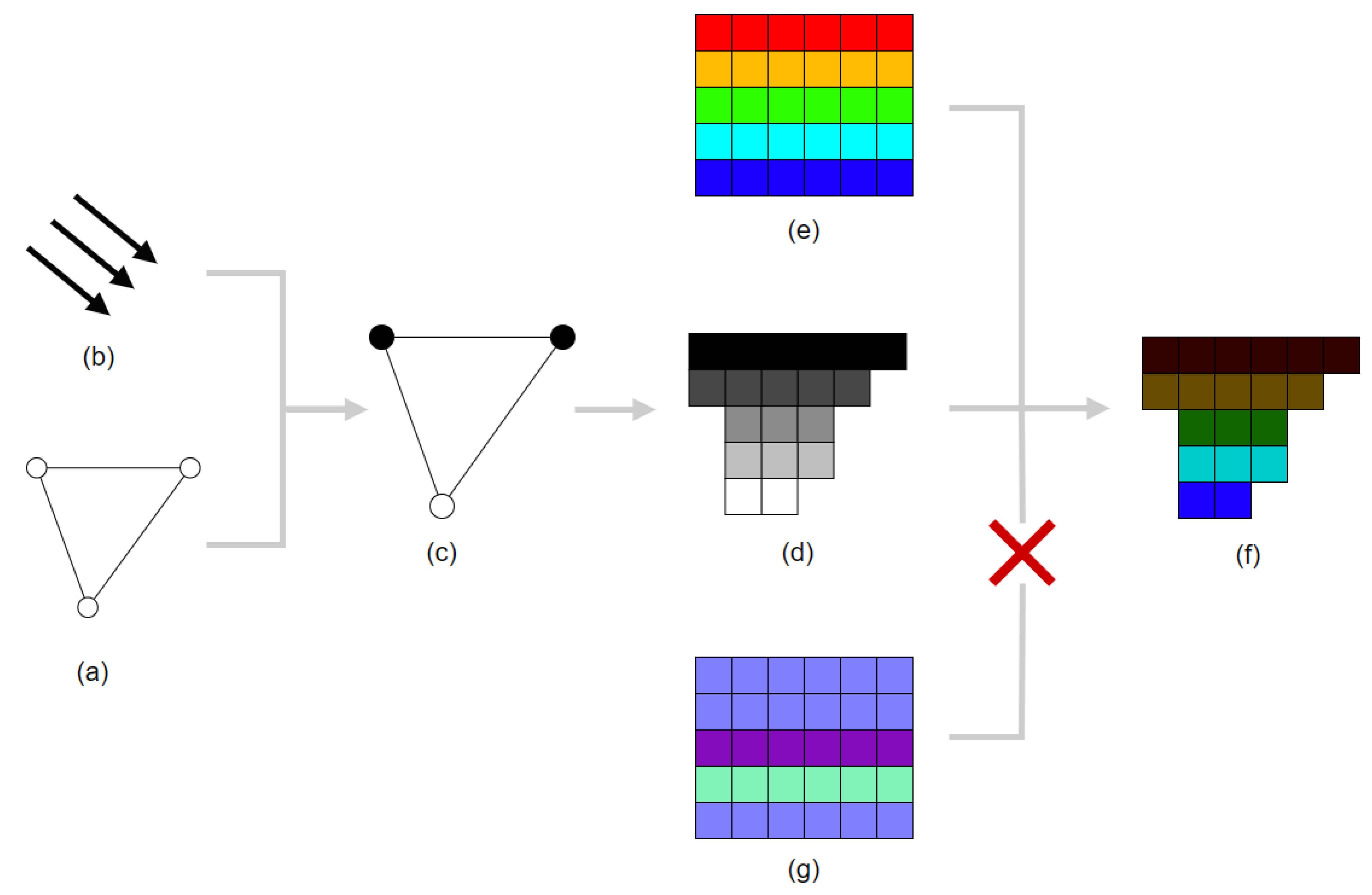
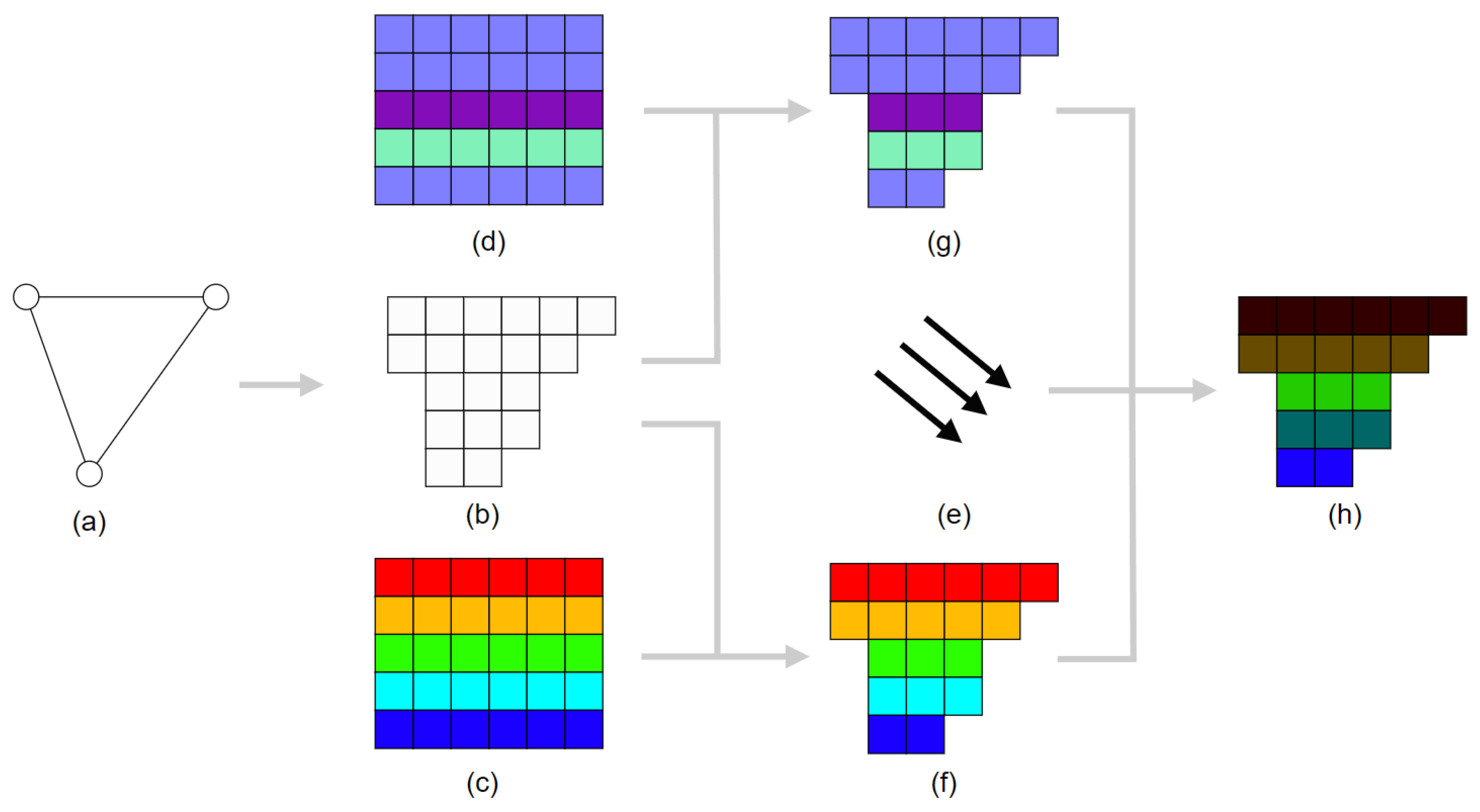
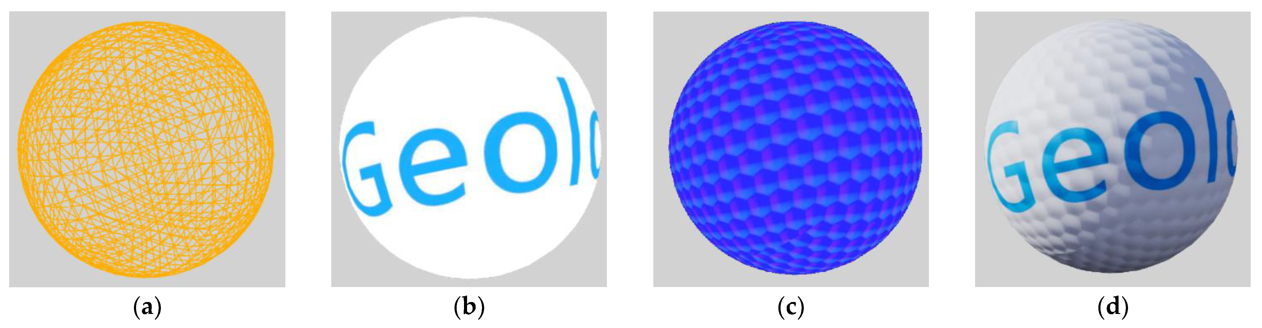
• Transformation and lighting. Here, vertices are transformed into camera space through model–view–projection (MVP) matrices. Then, for each vertex, a Blinn–Phong model is used to calculate the lighting of each vertex, which is called “per-vertex lighting” (Figure 1c);
• Primitive assembly. According to the vertex sequence specified by the application, the vertices are connected to the surfaces of triangles, which become faces or bodies with a polygonal topology structure (Figure 1c);
• Rasterization. Each triangle made in the last stage is rasterized into pixels. For each pixel, the Gouraud shading algorithm is used to interpolate the lighting and UV coordinates of vertices around each pixel. At this stage, the per-vertex data become per-pixel data (Figure 1d);
• Texture mapping. Diffuse textures provided by the application are sampled according to the UV coordinates of each pixel. Then, at each pixel, the diffuse color multiplies the lighting to obtain the final color (Figure 1f).

Because all functions of FFPs are made possible by the exact design of the integrated circuit, adding new rendering algorithms means designing and manufacturing new chips, i.e., FFPs are non-programmable, which severely limits the evolution of rendering techniques. For example, normal mapping is a common texture mapping technique used for faking the lighting of bumps and dents, even in traditional offline rendering, but is not applicable in real-time rendering based on an FFP, as shown in Figure 1. This is because the lighting is calculated per vertex rather than per pixel. Without normal mapping, “virtual” 3D graphics are far from “reality”, like the golf ball in Figure 2.

Industries, especially the gaming industry, are always in pursuit of photo-realistic graphics. Thus, the FFP quickly became inadequate and faded into history. In 1999, the release of Nvidia’s graphics accelerator, GeForce 256, marked the end of FFPs and the advent of the era of programmable pipelines (PPs), which were backed by a new type of chip called the graphics processing unit (GPU) [25]. Together with CPUs, GPUs define the computing power of machines. Currently, GPUs are very different from CPUs in many ways. CPUs were initially designed to achieve better performance with higher frequency. But, since their introduction, GPUs have relied on the power of multiple cores. GPUs implement “single instruction–multiple data (SIMD)” to achieve high-performance parallel computing. Though modern CPUs are also multi-core, GPUs still have far more cores. For example, the Fermi architecture released in 2009 has 512 cores [25], which is a number still not achievable by CPUs in the 2020s. When rendering, each core of the GPU runs mathematical algorithms on each vertex, pixel, etc., by executing code snippets called “shaders”.

The reason why GPUs can render the same quality graphics at a much higher speed than traditional offline rendering running on CPUs is their special SIMD architecture, meaning that traditional CPU-based algorithms are no longer applicable on GPUs. On this SIMD architecture, all cores must execute the same instruction at the same time, though each core can have different data. This means that ordinary branching on GPUs might have greater overhead than CPUs. Consider the C code in Algorithm 1:

Line 0	if (a < b) {
Line 1	a * b;
Line 2	} else {
Line 3	a + b;
Line 4	}

On a multi-core CPU, which is normally “multiple instruction–multiple data (MIMD)” architecture, if line zero is TRUE on core-0 but FALSE on core-1, core-0 will then jump to line one, while core-1 will jump to line three at the next cycle without any overhead. But, with a GPU, no matter the result of line zero, all cores will jump to line one simultaneously and then jump to line three. Then, for each core, only the result that fulfills line zero will be picked, and the others are discarded. This is called “flattening” of branches. It is obvious that all cores perform useless computation at least once, wasting clock cycles. This example explains one of the reasons algorithms must be rewritten to fit to SIMD, but only specific types of algorithms can benefit from it. Fortunately, bitmap processing is naturally SIMD-friendly, so GPUs have become the best practice for SIMD architecture [26].

GPUs soon began to change real-time rendering from traditional “fixed” to modern “programmable”, allowing new algorithms to be introduced into the rendering pipeline. The normal mapping problem we mentioned above was solved by the first programmable graphics accelerator, Nvidia’s GeForce 3, marking a great leap in real-time graphics rendering [25]. Figure 3 demonstrates how modern PPs handle rendering with the support of normal mapping using a software approach called “deferred rendering” [27], in contrast to the traditional “forward rendering” of an FFP. In deferred rendering, vector data become rasterized as soon as possible, resulting in a group of special bitmaps called a G-buffer. The final image is then calculated per pixel from the G-buffer. With normal mapping, the same golf ball model shows a much better result in Figure 4.

Due to the programmability of GPUs, they are no longer mere graphics processing devices but the most widely used parallel computing platforms. In 2003, two independent research groups discovered that using GPUs to solve general linear algebra problems is more efficient than using CPUs [28], opening the prelude to general purpose GPU (GPGPU) computing. Nowadays, GPGPUs have become an important foundation for various cutting-edge computations, e.g., artificial intelligence and virtual simulation.

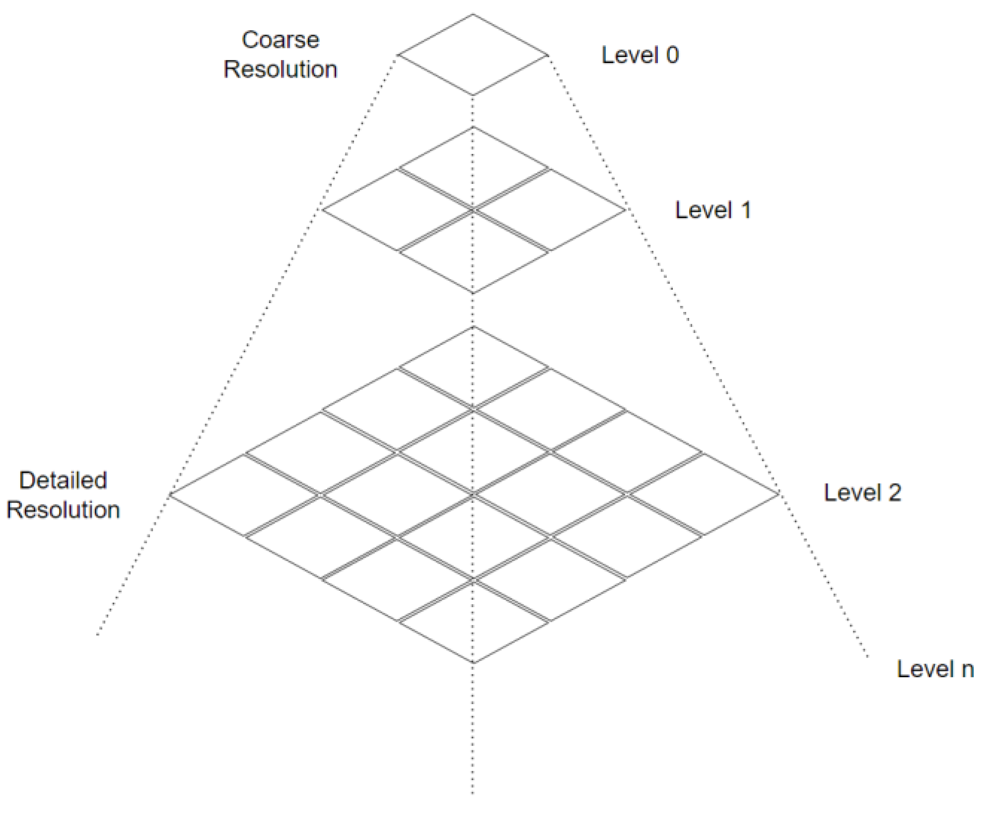
2.3. Tiled Web Map

Although the medium for maps evolved from Turin Papyrus Map’s papyrus to clay tablets, wooden boards, silk, and, eventually, paper, the scope and accuracy of these kinds of physical maps were always limited by the area of the medium itself. Roger Tomlinson developed the world’s first geographics information system, the Canada Geographic Information System [29], ushering in the era of digital maps. However, due to the limitations of computer performance, many early digital maps had the same limitations as paper maps, and, thus, the amount of detail is limited by the size of the map. To overcome this limitation, Google invented the “slippy map”, also known as the “tiled map”, paving the way for modern web maps [30].

Tiled maps divide the world map into several “zoom levels” according to the map scale, and each level of the map is divided into several equally sized square tiles. These tiles are combined in a quadtree from the lowest level to the highest level, like a pyramid, as shown in Figure 5. When users browse the map, the program automatically selects the most suitable tiles for loading based on the area and resolution viewed by the user, allowing the users to use natural manipulations, such as dragging, rotating, and zooming, to continuously view global geographic information without having to switch between different map regions and scales, like with physical maps.

Taking Google Maps as an example, its tiled map service for third parties divides world imagery into 20 levels, and each level is divided into JPEG images with a resolution of 256 × 256 pixels according to the WGS84 system (EPSG:4326). Each level has $4^n$ tiles, where $n$ is the level number. These tiles can be accessed through the TMS and WMTS protocols. Any third-party program that supports these protocols can use Google Maps’ tiled map data.

In 2011, to visualize spatial objects based on tiled maps in 3D space, developers at Analytical Graphics made a 3D globe program called Cesium, which became open-source in 2012. Since then, the Cesium team has led and participated in many technological innovations related to 3D global maps, such as co-developing the glTF format with the Khronos Group, which has become a fundamental real-time 3D model format standard, and inventing the 3D Tiles format, which has become the OGC Community Standard for large-scale 3D data streaming. Thanks to its open-source and cross-platform nature, Cesium has been widely used in scientific research [32], industries, and military fields, such as MathWorks, NORAD, Bentley Systems, OneGeology, and others.

The most used version of Cesium is CesiumJS, which provides the ability to use a 3D globe in a browser. However, to fully leverage the capabilities of modern GPUs, Cesium provides cesium-native to allow platform-native applications to use the full range of Cesium’s capabilities. For example, Cesium for Unreal, based on cesium-native, allows users to create a 3D globe based on the famous Unreal Engine (Figure 6). As one of the most powerful real-time rendering engines, the open-source Unreal Engine supports today’s most advanced GPU features, including real-time ray tracing. Cesium for Unreal can also fully utilize these features of the Unreal Engine, allowing users to develop GIS software based on modern real-time rendering technology [33].

3. A Novel Prospecting Evaluation Method

Vector data are not suitable for various parallel operations on GPUs. To leverage the computing power of modern GPUs, the data structure must change to bitmaps. As we mentioned above, data used in prospecting evaluation can be categorized as qualitative and quantitative, such as geological maps, which are qualitative, and geochemical maps, which are quantitative. Thus, we propose IGM and DGM contain these two types of data in bitmaps, allowing for computation on GPUs. Based on these two types of bitmaps, we developed a novel software system on top of Cesium for Unreal.

Due to the influence of the curvature of the earth, this system is currently mainly aimed at the work of large-scale regional prospecting evaluation; more algorithm development is needed on this basis for small-scale regions.

3.1. Dynamic Geochemical Maps (DGMs)

An important task in exploration geochemistry is to delineate anomalies—in other words, to highlight anomalies. In our practice of evaluating the Zhunuo geochemical anomalies, we found that, if we could tune the parameters in real time during the analysis, we could more easily understand the anomalies comprehensively. To fulfill this requirement, we proposed dynamic geochemical maps.

Here, we use the data of stream Cu sediment [34] from a regional geochemical survey conducted at a scale of 1:50,000 in the Zhunuo ore district to explain the creation and rendering of a DGM. A total of 1457 stream sediment samples used here were taken at a density of about 1 sample per 0.25 km² from areas at longitudes of 87°15′–87°30′ and latitudes of 29°30′–29°40′. The element Cu was analyzed using XRF (X-ray fluorescence). The statistical properties of the concentration of Cu are summarized in

Table 1. Statistical parameters of the geological data on the stream sediment element concentrations at a 1:50,000 scale in the Zhunuo ore district.

Element	Cu
Number of Samples	1457
Mean	0.63
Std	1.73
CV	2.75
Median	0.17
MAD	0.09
Minimum	0.03
Maximum	45.91
25th percentiles	0.10
75th percentiles	0.42
95th percentiles	3.07
98th percentiles	5.34
Skewness	14.08
Kurtosis	329.54

Note: The unit of Cu is ppm (10-6). Std means the standard deviation; CV means the coefficient of variation; MAD means the median absolute deviation.

.

The DGM was created and rendered through the following steps:

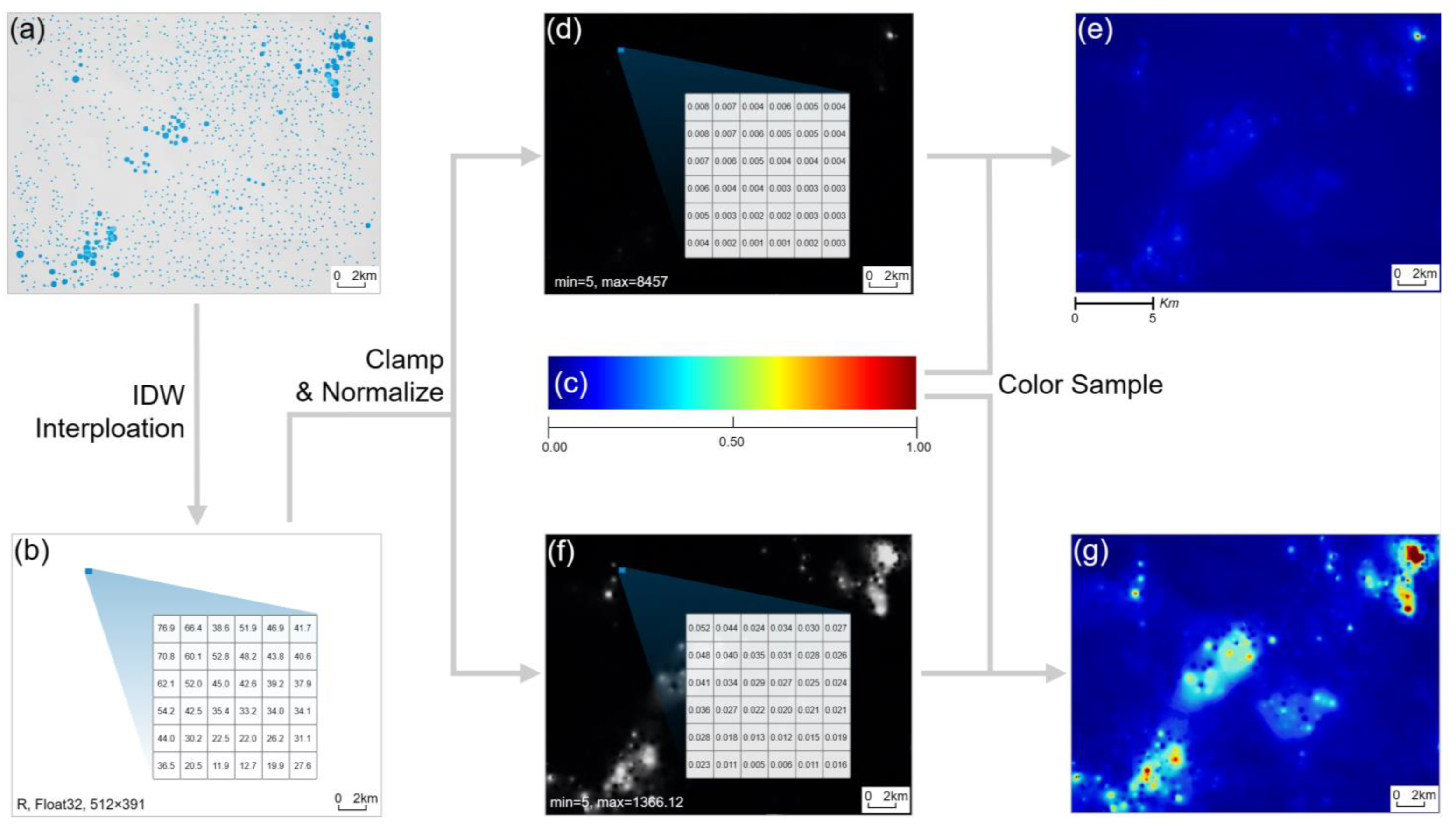
• We created a single-channel float format TIFF image with an aspect ratio equal to the Zhunuo ore district map’s frame with a maximum length of 512 pixels. The four corners of the image had corresponding geographic spatial coordinates that could be deduced from the ore district map. Here, we call this image the DATA.
• We used the inverse distance weight method to interpolate the Cu value to each pixel in this image, so each pixel stored the value at the spatial position to which each pixel corresponded, as shown in Figure 7b.
• We generated a 3-channel (RGB) 8-bit format image with a height of 1 pixel and a width of 1024 pixels and filled this image with a gradient of rainbow using OpenCV, as shown in Figure 7c. Here, we call this image the PALETTE.
• We loaded the above two images as textures into the video memory and used them in the rasterization layers of Cesium for Unreal.
• To render the DATA texture into the correct spatial position, an algorithm called “inverse bilinear interpolation” was used and is explained in detail later. In this step, the spatial position of every pixel in the DATA was determined by computing the UV coordinates of each pixel on the 3D globe for sampling the DATA.
• In the material of the rasterization layers of Cesium for Unreal, after sampling the DATA with the UV coordinates from the last step, the sampling value had to be transformed with the following algorithm to clamp and normalize, as follows:
  • Let $f(x,a,b)=\left\{\begin{array}{c}0, x<a\\ \frac{(x-a)}{(b-a)}, a\le x\le b\\ 1, x>b\end{array}\right.$, calculate $u=f(l,m,n)$, where $l$ is the sampling value, $m$ is the lower anomaly limit from the user input, and $n$ is the upper anomaly limit from the user input.
  • Use $(u,0)$ as the UV coordinates to sample the PALETTE, and then output the sampling color.
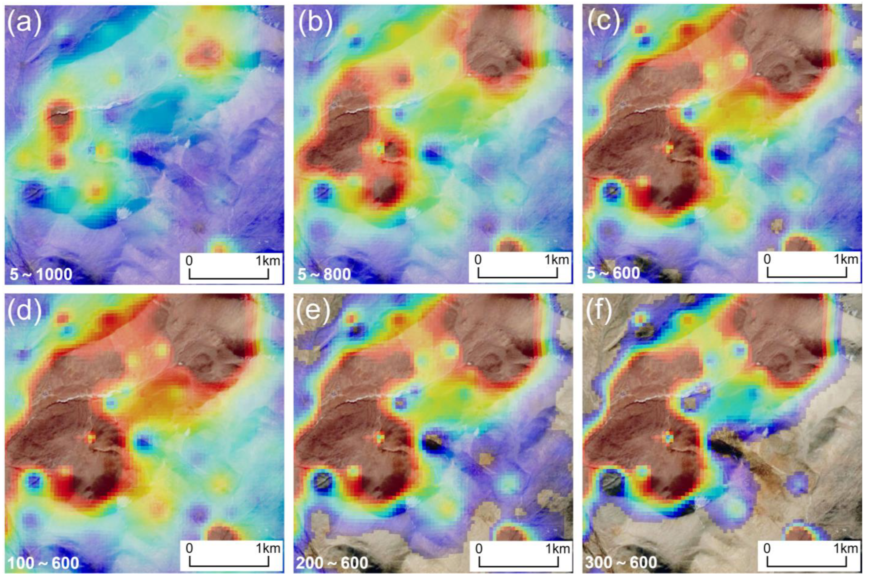
• Because GPUs can reflect changes in real time, by inputting different m and n, the upper and lower anomaly limits can be tuned in real time. As shown in Figure 7d,f using a different m and n resulted in different visualizations in Figure 7e,g. Each result was generated in less than 10 milliseconds on a GeForce RTX 3070 GPU.

3.2. Interactive Geological Map (IGM)

Geological maps are the most used maps to convey qualitative data in comprehensive regional prospecting evaluations. In traditional vector maps, lithology data are stored as “attributes” in each vector region, where lithology is essentially a text description. Text is not practical to store in each pixel due to the characteristics of bitmap formats. However, considering that the lithology in a single prospecting region is usually limited, we can use enumeration and key-value mapping to store lithology, and that is the core logic of interactive geological maps. IGMs focus on achieving three goals: (1) distinguishing various lithology regions on the terrain by color; (2) being able to control the visibility of each lithology region separately; (3) being able to query the lithology of each region with a mouse in real time.

An IGM of the Zhunuo ore district was created and rendered through the following steps:

• All lithology descriptions in the original vector geological map were counted and numbered in order using a Python script. These lithology descriptions were stored in a key-value map, as shown in

  Table 2. The key-value map of lithology in the Zhunuo ore district.

  Number	Lithology Description
  1	Diorite
  2	Monzonite porphyry
  3	N1—Biotite monzogranite porphyry
  4	N1—Medium-coarse-grained porphyritic biotite monzogranite
  5	E2—Upper Pana Formation
  6	E2—Lower Nianbo Formation
  7	N1—Medium-fine-grained porphyritic granite porphyry
  8	E2—Medium-fine-grained biotite granodiorite
  9	E1—Upper Dianzhong Formation
  10	N1—Porphyritic monzogranite
  11	E2—Medium-coarse-grained biotite monzogranite
  12	N1—Medium-coarse-grained porphyritic biotite monzogranite
  13	E2—Medium-fine-grained K-feldspar granite
  14	E2—Upper Pana Formation
  15	E2—Lower Nianbo Formation
  16	N1—Porphyritic monzogranite
  17	E2—Medium-coarse-grained biotite monzogranite

  . This table was serialized to a JSON file as an object, as shown in Figure 8g.

2.

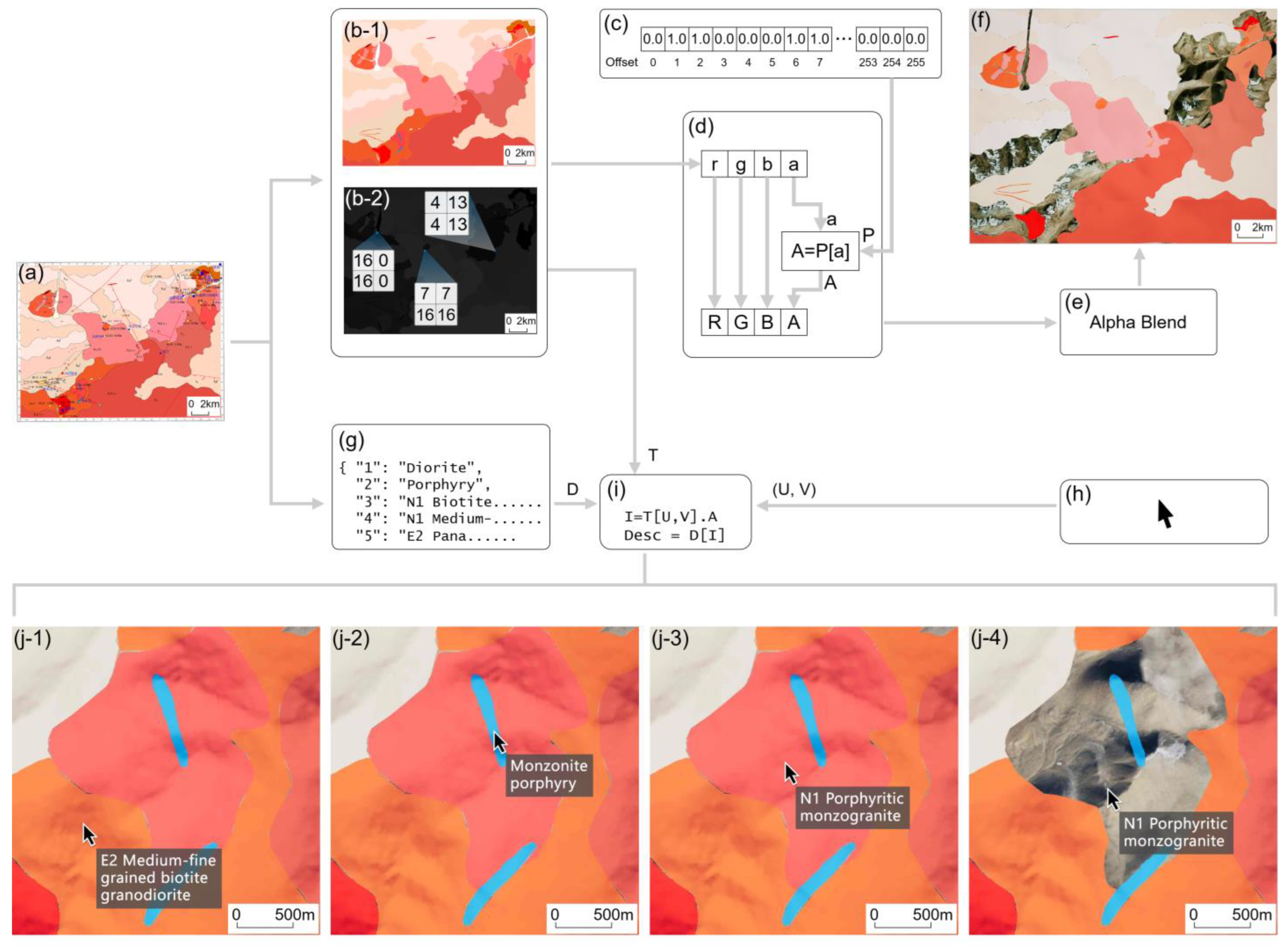
We rasterized the lithology regions in the vector geological map. During the rasterization process, the RGB colors were written into the image’s RGB channel, and the region numbers from the enumeration were written into the alpha channel, as shown in Figure 8(b-1,b-2). All four channels were in unsigned int-8 format. Here, we call this image the DATA.

3.

The map region of Zhunuo is a convex quadrilateral but not a rectangle, and GPU rendering requires that textures must be rectangular. Therefore, the DATA had to be perspective-corrected and clipped in OpenCV to fill an entire rectangular image, just like the DGM we just created.

4.

As we mentioned above, the visibility of the lithology regions must be controllable separately. To achieve this, the application procedurally created an image with a width of 256 pixels, as each pixel corresponded to a type of lithology, as shown in Figure 8c. Here, we call this image the LUT. Users can control the visibility by changing the values of these pixels. For example, if the user wants to make “monzonite porphyry” visible, which has a numbering of two according to Table 2, they can simply set the third pixel from the left of the LUT, whose index is two in a zero-based numbering, to a value of 1.0 in a linear space (which is 255 in a non-linear unsigned int-8 space). In contrast, it needs to be set to 0.0 if the user wants to make it invisible.

Figure 8. The creation, rendering, and querying of the interactive geological map of Zhunuo. (a) The original vector geological map. (b-1,b-2) The image converted from (a) as the RGB channel; (b-1) contains color and the alpha channel, and (b-2) contains the enumeration of the lithology. (c) The image was 256 pixels wide, 1 pixel high to control the visibility of each type of lithology. (d) The algorithm to control the visibility of each pixel. (e) Alpha blending was used to compose the background satellite imagery with the IGM. (f) The final image. (g) The JSON object containing the enumeration mapping of the lithology description. (h) The coordinates of the mouse cursor converted to the UV coordinates corresponding to the IGM. (i) The algorithm to obtain the lithology description of the region under the cursor. (j-1–j-4) As the cursor moves, the lithology under the cursor is reported in real time.

Figure 8. The creation, rendering, and querying of the interactive geological map of Zhunuo. (a) The original vector geological map. (b-1,b-2) The image converted from (a) as the RGB channel; (b-1) contains color and the alpha channel, and (b-2) contains the enumeration of the lithology. (c) The image was 256 pixels wide, 1 pixel high to control the visibility of each type of lithology. (d) The algorithm to control the visibility of each pixel. (e) Alpha blending was used to compose the background satellite imagery with the IGM. (f) The final image. (g) The JSON object containing the enumeration mapping of the lithology description. (h) The coordinates of the mouse cursor converted to the UV coordinates corresponding to the IGM. (i) The algorithm to obtain the lithology description of the region under the cursor. (j-1–j-4) As the cursor moves, the lithology under the cursor is reported in real time.

5.

We loaded the DATA and the LUT as textures into the video memory and used them in the rasterization layers of Cesium for Unreal. Just like the DGM, to render the DATA in the correct spatial position, we needed to compute the UV coordinates of each pixel on the 3D globe for sampling the DATA using “inverse bilinear interpolation” too, which is explained in detail later.

6.

In the material of the rasterization layers of Cesium for Unreal, after sampling the DATA with the UV coordinates from last step, a four-component array representing RGBA color in the linear space was obtained. Among them, A represents the numbering of the lithology corresponding to the pixel, which is also the U component of the UV coordinates to sample the visibility of this lithology type in the LUT. If the sampling value from the LUT is greater than 0.0, then the sampling color from the DATA is the RGB component output. Otherwise, the color is output in the next layer, as this specified lithology is invisible, as shown in Figure 8d–f.

7.

To interactively query the lithology description at each place, the 3D world coordinates corresponding to the mouse cursor on the 3D terrain must be acquired first. Here, again, we used “inverse bilinear interpolation” to calculate the UV coordinates of the cursor position relative to the four corners of the IGM. On the CPU side of the application, we used these UV coordinates to sample the DATA to obtain the lithology numbering at the position, just like on the GPU side. With the lithology numbering, we queried the key-value map in the JSON format we made above to obtain the lithology description, as shown in Figure 8(j-1–j-4).

3.3. Inverse Bilinear Interpolation

As mentioned above, both DGMs and IGMs use inverse bilinear interpolation to render textures into correct spatial positions. Inverse bilinear interpolation is an algorithm to calculate the UV coordinates at any position inside a convex quadrilateral if all coordinates we know are in world space [35]. Thus, with this algorithm, we can map every pixel inside of the ore district to a pixel in the DGM or the IGM. The definition of inverse bilinear interpolation is as follows:

Consider a convex quadrilateral made of four vertices, $\overrightarrow{a}$, $\overrightarrow{b}$, $\overrightarrow{c}$, and $\overrightarrow{d,}$ in 2D space, and let $\overrightarrow{p}$ be a point inside of it, as follows:

$$\overrightarrow{p}=〈p_1,p_2〉, \overrightarrow{a}=〈a_1,a_2〉, \overrightarrow{b}=〈b_1,b_2〉, \overrightarrow{c}=〈c_1,c_2〉, \overrightarrow{d}=〈d_1,d_2〉$$

(1)

Then, the UV coordinates of $\overrightarrow{p}$ are as follows:

$$v=\frac{2k_0}{-k_1-\sqrt{{k_1}^2-4k_0{k}_2}}, u=\frac{p_1-a_1-d_{1}v+a_{1}v}{b_1-a_1+a_{1}v-b_{1}v+c_{1}v-d_{1}v}$$

(2)

The intermediate variables are as follows:

$$k_0=\left(\overrightarrow{p}-\overrightarrow{a}\right)\times \left(\overrightarrow{b}-\overrightarrow{a}\right)$$

(3)

$$k_1=\left(\overrightarrow{b}-\overrightarrow{a}\right)\times \left(\overrightarrow{d}-\overrightarrow{a}\right)+\left(\overrightarrow{p}-\overrightarrow{a}\right)\times \left(\overrightarrow{a}-\overrightarrow{b}+\overrightarrow{c}-\overrightarrow{d}\right)$$

(4)

$$k_2=\left(\overrightarrow{a}-\overrightarrow{b}+\overrightarrow{c}-\overrightarrow{d}\right)\times \left(\overrightarrow{d}-\overrightarrow{a}\right)$$

(5)

Inverse bilinear interpolation, which can be used in a shader, establishes the mathematical foundation for the accurate spatial mapping of images on GPUs. In our system’s implementation, we first converted the latitude and longitude coordinates of the image corners into the 3D space rectangular coordinates of Unreal and then passed these coordinates through the Material Parameter Collection (which is a container in Unreal Engine for uniform variables in shaders) to Cesium’s layered material. In the material, the inverse bilinear interpolation algorithm was implemented using High-Level Shader Language (HLSL), where $\overrightarrow{p}$ represents the XY components of the world coordinates of the pixel, and $\overrightarrow{a}$, $\overrightarrow{b}$, $\overrightarrow{c}$, and $\overrightarrow{d}$ represent the XY components of the image corner coordinates passed from the Material Parameter Collection. After running the algorithm, the UV coordinates were acquired.

Inverse bilinear interpolation is also used in the real-time query of lithology in the IGM. But, different from the same algorithm implemented in a shader, i.e., on the GPU side, the one used in this query is implemented on the CPU side, and $\overrightarrow{p}$ represents the XY components of the coordinates of the mouse projected onto the 3D terrain.

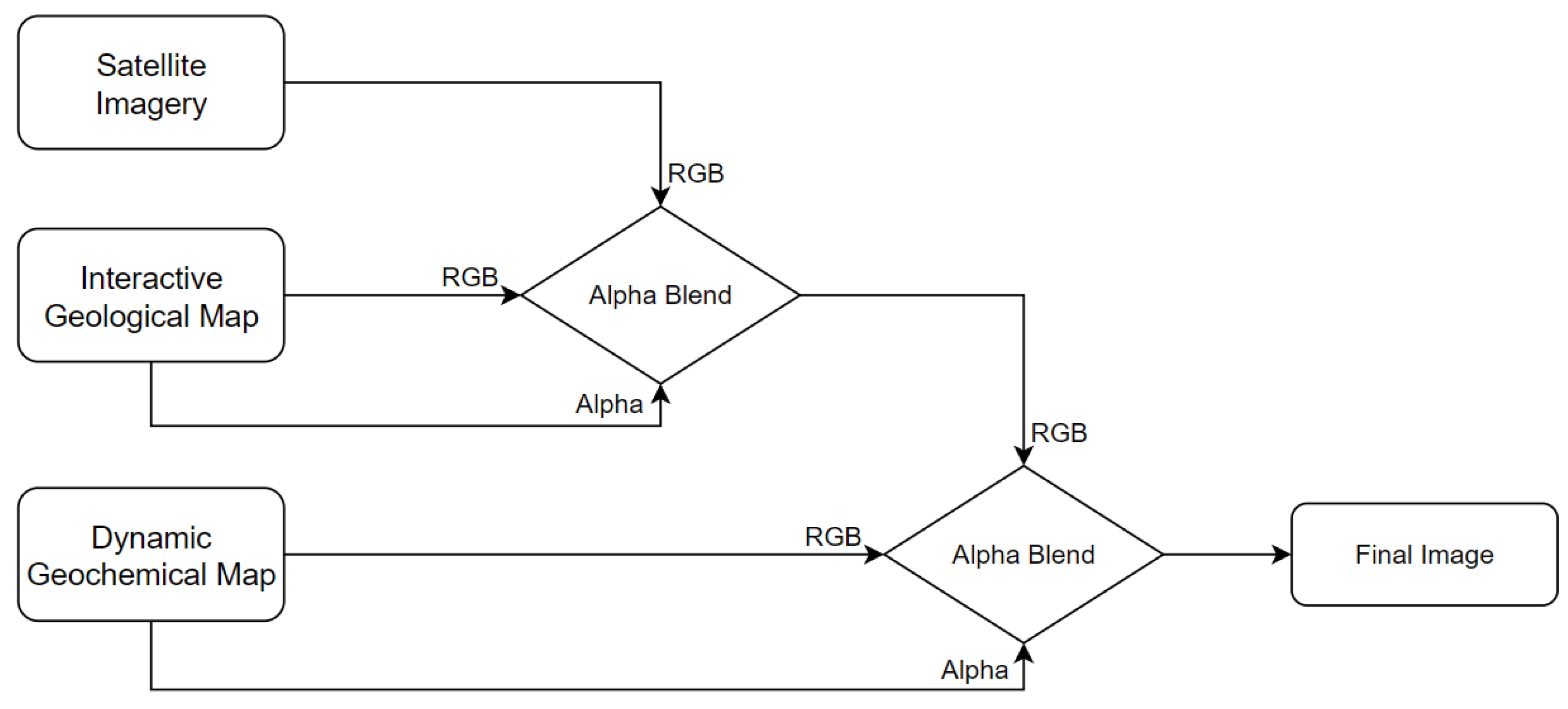
3.4. Composition of Bitmaps

In the work of prospecting evaluation, the two maps described above need to be combined with satellite imagery in real time. Cesium uses Unreal Engine’s layered material system to achieve multi-layer composition. In this layered material, the satellite imagery is used as the bottom layer, and then the IGM and DGM are overlayed on top of it through alpha blending, as shown in Figure 9. After the composition, three layers of bitmaps become the final image and are then mapped on to the 3D globe.

4. Practice in the Zhunuo Ore District

With the methods described above, we made a novel software system with multiple features (Figure 10) and used it in the prospecting evaluation of the Zhunuo ore district, which is located at the western section of the Gangdese metallogenic belt in Tibet. The area has significant geochemical anomalies with a high degree of element enrichment. Many mineral deposits, mineralized bodies, and mineralization clues have been discovered. In the early stage of exploration, trenching and drilling work was carried out. However, except for the Zhunuo and Beimumu copper deposits, the effect of further exploration was not significant, and the ore bodies were discontinuous on the surface and not scaled. The reason may be that the real anomaly center has not been delineated [36,37]. For example, in the Dongshibu-Hongshan area, which invested a lot of exploration funds in the early stage, although the geochemical anomalies were relatively high, no ore bodies were found after drilling verification. This article’s invented method was applied to process the geochemical data of the Zhunuo ore district, draw a Cu element anomaly map, and superimpose it on the geological map to form a comprehensive mineral exploration analysis system that displays Cu element anomalies and mineralized geological bodies in real time and dynamically with three-dimensional terrain in the Zhunuo district (Figure 11). After analysis, it was found that the Hongshan area where drilling was originally carried out was not the anomaly center, and the real anomaly center was located in the northeast. Therefore, when using traditional methods to delineate anomalies, one must be cautious and consider the topographic effects and geological background comprehensively (Figure 12). It can be seen that using this method can not only greatly improve the efficiency of geochemical data processing but can also avoid the economic losses caused by misjudgment of mineralization clues and reduce exploration costs and risks, which has important promotion value and demonstration significance.

5. Discussion

Our proposed method involves dynamic geochemical maps and interactive geological maps in bitmap format corresponding to traditional vector geochemical maps and geological maps, allowing researchers to conduct comprehensive regional prospecting evaluations in real time on a 3D globe and map to determine the relationships among the terrain, geology, and geochemistry. With this method, GPUs are used to realize the real-time adjustment of geochemical anomalies, achieving tuning-while-evaluating. Traditionally, the combination of geographic data is completed through vector format graphics in 2D space. Our method uses the inverse bilinear interpolation algorithm to accurately overlay bitmaps on the 3D globe, enabling data to be represented by GPU-friendly bitmaps instead of traditional GPU-unfriendly vector graphics, laying the foundation for unleashing the computing power of GPUs. A novel software system based on these methods was tested in practice in the prospecting evaluation of the Zhunuo ore district, proving its advantages over traditional vector graphics-based software.

Initially, we mainly focused on the DGM to visualize geochemical data in 3D space in real time. However, in actual practice, it was found that combining them with geological data is also crucial. After analyzing the data needs of researchers and the characteristics of geological maps, we realized that regional geological data are essentially a type of enumeration. Therefore, we implemented a method of storing regional geological data using bitmaps and JSON objects. And, again, with the help of inverse bilinear interpolation algorithm, we implemented the real-time querying of geological data in the IGM.

However, the software system is still in its early stages, and there is still a lot of room for improvement. For example, the working area of this system is generally limited to an area corresponding to a large-scale paper map, because the inverse bilinear interpolation algorithm assumes that the interpolation target is a plane, which is similar to the limitation of the Gauss–Krüger and Transverse Mercator projections. To apply this method to areas with smaller scales, algorithms must be studied to address the earth’s curvature.

In addition, the system currently only implements the visualization of geochemical data and geological data. However, prospecting evaluation works usually require the use of remote sensing data, geophysical data, etc., which can also be classified as “quantitative”. Therefore, we can extend the method used, implementing the DGM, to visualize those data and thus to enhance the system’s capabilities.

6. Conclusions

The software system we developed based on the method in this study currently allows researchers to combine geochemical maps and geological maps on a 3D globe and map to achieve comprehensive regional prospecting evaluation in 3D space in real time. Unlike existing software systems that mainly rely on vector data, our system is totally based on bitmap data. Therefore, our system can fully utilize the computing advantages of modern GPUs. Based on the computing power of the GPU, we implemented the dynamic geochemical map, allowing researchers to tune while evaluating in real time. And, in order to combine geological data, we also implemented the interactive geological map, which allows researchers to analyze geological data on a 3D globe and map. The system was first applied to a prospecting evaluation in the Zhunuo ore district, demonstrating the advantages of our method. Researchers working in the Zhunuo ore district recognized the advantages of our system but also found its limitations, such as its limited map scale and data types. We will continue to optimize the features and algorithms based on feedback from researchers to overcome these problems and make the system more applicable in future developments.

References

- Carranza, E.J.M. Geochemical Anomaly and Mineral Prospectivity Mapping in GIS; Elsevier: Amsterdam, The Netherlands, 2008. [Google Scholar]
- Zuo, R.; Carranza, E.J.M.; Wang, J. Spatial analysis and visualization of exploration geochemical data. Earth Sci. Rev. 2016, 158, 9–18. [Google Scholar] [CrossRef]
- Zuo, R.; Wang, J.; Xiong, Y.; Wang, Z. The processing methods of geochemical exploration data: Past, present, and future. Appl. Geochem. 2021, 132, 105072. [Google Scholar] [CrossRef]
- Cheng, Z.; Xie, X.; Yao, W.; Feng, J.; Zhang, Q.; Fang, J. Multi-element geochemical mapping in Southern China. J. Geochem. Explor. 2014, 139, 183–192. [Google Scholar] [CrossRef] [PubMed]
- Cheng, Q. Spatial and scaling modelling for geochemical anomaly separation. J. Geochem. Explor. 1999, 65, 175–194. [Google Scholar] [CrossRef]
- Desktop GIS Software. Available online: https://www.esri.com/en-us/arcgis/products/arcgis-pro/overview (accessed on 15 March 2024).
- Yin, B.; Zuo, R.; Xiong, Y.; Li, Y.; Yang, W. Knowledge discovery of geochemical patterns from a data-driven perspective. J. Geochem. Explor. 2021, 231, 106872. [Google Scholar] [CrossRef]
- Nowak, M.M.; Dziób, K.; Ludwisiak, Ł.; Chmiel, J. Mobile GIS applications for environmental field surveys: A state of the art. Glob. Ecol. Conserv. 2020, 32, e01089. [Google Scholar] [CrossRef]
- Global Mapper. Available online: https://www.bluemarblegeo.com/global-mapper/ (accessed on 15 March 2024).
- Image Processing & Analysis Software. Available online: https://www.nv5geospatialsoftware.com/Products/ENVI (accessed on 15 March 2024).
- Xing, Y.; Gomez, R.B. Hyperspectral image analysis using ENVI (environment for visualizing images). In Proceedings of the SPIE—The International Society for Optical Engineering, Orlando, FL, USA, 16–20 April 2001. [Google Scholar] [CrossRef]
- Zuo, R.; Yin, B. Google Earth-aided visualization and interpretation of geochemical survey data. Geochem. Explor. Environ. Anal. 2022, 22, 125959. [Google Scholar] [CrossRef]
- Earth Versions—Google Earth. Available online: https://www.google.com/earth/about/versions/ (accessed on 15 March 2024).
- Ovital Interactive Map (In Chinese). Available online: https://www.ovital.com/download/ (accessed on 15 March 2024).
- Asano, S.; Maruyama, T.; Yamaguchi, Y. Performance comparison of FPGA, GPU and CPU in image processing. In Proceedings of the 2009 International Conference on Field Programmable Logic and Applications, Prague, Czech Republic, 31 August–2 September 2009. [Google Scholar] [CrossRef]
- Zheng, Y.; Gao, S.; Zhang, D.; Fan, Z.; Zhang, G.; Ma, G. The discovery of the Zhunuo porphyry copper deposit in Tibet and its significance. Earth Sci. Front. 2006, 13, 233–239. (In Chinese) [Google Scholar]
- Zheng, Y.; Sun, X.; Gao, S.; Wang, C.; Zhao, Z.; Wu, S.; Li, J.; Wu, X. Analysis of stream sediment data for exploring the Zhunuo porphyry Cu deposit, southern Tibet. J. Geochem. Explor. 2014, 143, 19–30. [Google Scholar] [CrossRef]
- Google Maps Tile API. Available online: https://developers.google.com/maps/documentation/tile (accessed on 15 March 2024).
- Harrell, J.A.; Brown, V.M. The World’s oldest surviving geological map: The 1150 BC Turin Papyrus from Egypt. J. Geol. 1992, 100, 3–18. [Google Scholar] [CrossRef]
- Blackborow, J. Digital Experiences in the Physical World; Forrester: Cambridge, MA, USA, 2020. [Google Scholar]
- Kontkanen, J. Novel Illumination Algorithms for Off-Line and Real-Time Rendering. Ph.D. Thesis, Helsinki University of Technology, Helsinki, Finland, 9 February 2007. [Google Scholar]
- Eevee vs. Cycles (CPU Rendering) Comparison on a Mac. Available online: https://blenderartists.org/t/eevee-vs-cycles-cpu-rendering-comparison-on-a-mac/1275653 (accessed on 15 March 2024).
- Hadwiger, M. 3D Graphics Technology in Computer Games Past, Present, and Future. In Proceedings of the 4th Central European Seminar on Computer Graphics, Budmerice, Slovakia, 3 May 2000. [Google Scholar]
- Holmåker, M.; Woxblom, M. Performance evaluation of the fixed function pipeline and the programmable pipeline. Master’s Thesis, Blekinge Institute of Technology, Blekinge, Sweden, 24 June 2004. [Google Scholar]
- Nickolls, J.; Dally, W.J. The GPU computing era. IEEE Micro. 2010, 30, 56–69. [Google Scholar] [CrossRef]
- Cypher, R.; Sanz, J.L. SIMD architectures and algorithms for image processing and computer vision. IEEE Trans. Acoust. Speech. Signal. Process. 1989, 37, 2158–2174. [Google Scholar] [CrossRef]
- Thaler, J. Deferred Rendering; TU Wein: Vienna, Austria, 2011. [Google Scholar]
- Krüger, J.; Westermann, R. Linear algebra operators for GPU implementation of numerical algorithms. In Proceedings of the ACM SIGGRAPH 2005 Courses, Los Angeles, CA, USA, 4 August 2005. [Google Scholar] [CrossRef]
- Fisher, T.; MacDonald, C. An Overview of the Canada Geographic Information System (CGIS); Lands Directorate Environment Canada: Ottawa, ON, Canada, 1980. [Google Scholar]
- Crampton, J.W. Keyhole, Google Earth, and 3D Worlds: An Interview with Avi Bar-Zeev. Cartogr. Int. J. Geogr. Inf. Geovis. 2008, 43, 85–93. [Google Scholar] [CrossRef]
- García, R.; de Castro, J.P.; Verdú, E.; Verdú, M.J.; Regueras, L.M. Web map tile services for spatial data infrastructures: Man-agement and optimization. In Cartography—A Tool for Spatial Analysis; Bateira, C., Ed.; InTech: Rijeka, Croatia, 2012; pp. 26–48. [Google Scholar] [CrossRef]
- Gede, M. Thematic mapping with Cesium. In Proceedings of the 6th International Conference on Cartography and GIS, Albena, Bulgaria, 20–25 June 2016. [Google Scholar]
- Hu, W.; Liu, D.; You, P.; Zhao, J.; Du, H.; Zhang, H. Research on Digital Governance of Rural Environment Based on Cesium for Unreal. In Proceedings of the 1st International Conference on Public Management, Digital Economy and Internet Technology, Changsha, China, 23–25 September 2022. [Google Scholar]
- Ci, Q.; Liu, X.; Zhu, J.; Basang, C.; Jia, C.; Wujian, C.; Xirao, J.; Basang, O.; Dawa, Z. Report of Mineral Prospecting Survey in the Zhunuo Area, Tibet; Geological Survey Bureau: Lhasa, Tibet, China, 2009. (In Chinese) [Google Scholar]
- Inigo Quilez: Computer Graphics, Mathematics, Shaders, Fractals, Demoscene and More. Available online: https://iquilezles.org/articles/ibilinear (accessed on 20 December 2023).
- Zheng, Y.; Zhang, G.; Xu, R.; Gao, S.; Pang, Y.; Cao, L.; Du, A.; Shi, Y. Geochronologic constraints on magmatic intrusions and mineralization of the Zhunuo porphyry copper deposit in Gangdese, Tibet. Chin. Sci. Bull. 2007, 52, 3139–3147. [Google Scholar] [CrossRef]
- Zheng, Y.; Wu, S.; Ci, Q.; Chen, X.; Gao, S.; Liu, X.; Jiang, X.; Zheng, S.; Li, M.; Jiang, X. Cu-Mo-Au Metallogenesis and Minerogenetic Series during Superimposed Orogenesis Process in Gangdese. Earth Sci. 2021, 46, 1909–1940. [Google Scholar] [CrossRef]