
Beneficiation of High-Density Tantalum Ore in the REFLUX™ Concentrating Classifier Analysed Using Batch Fractionation Assay and Density Data


Abstract
1. Introduction
2. Materials and Methods
2.1. The Tantalum Ore Feed
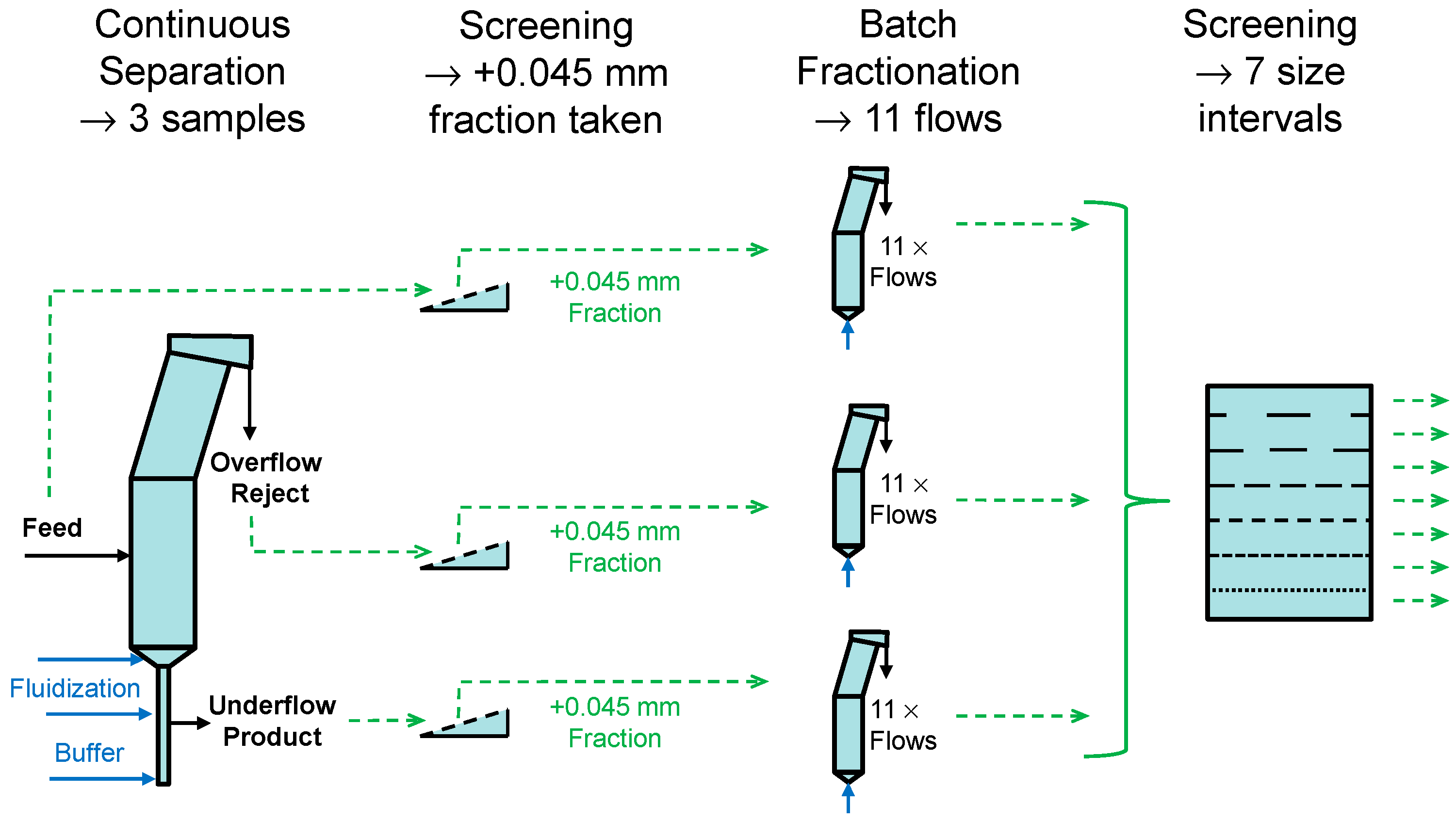
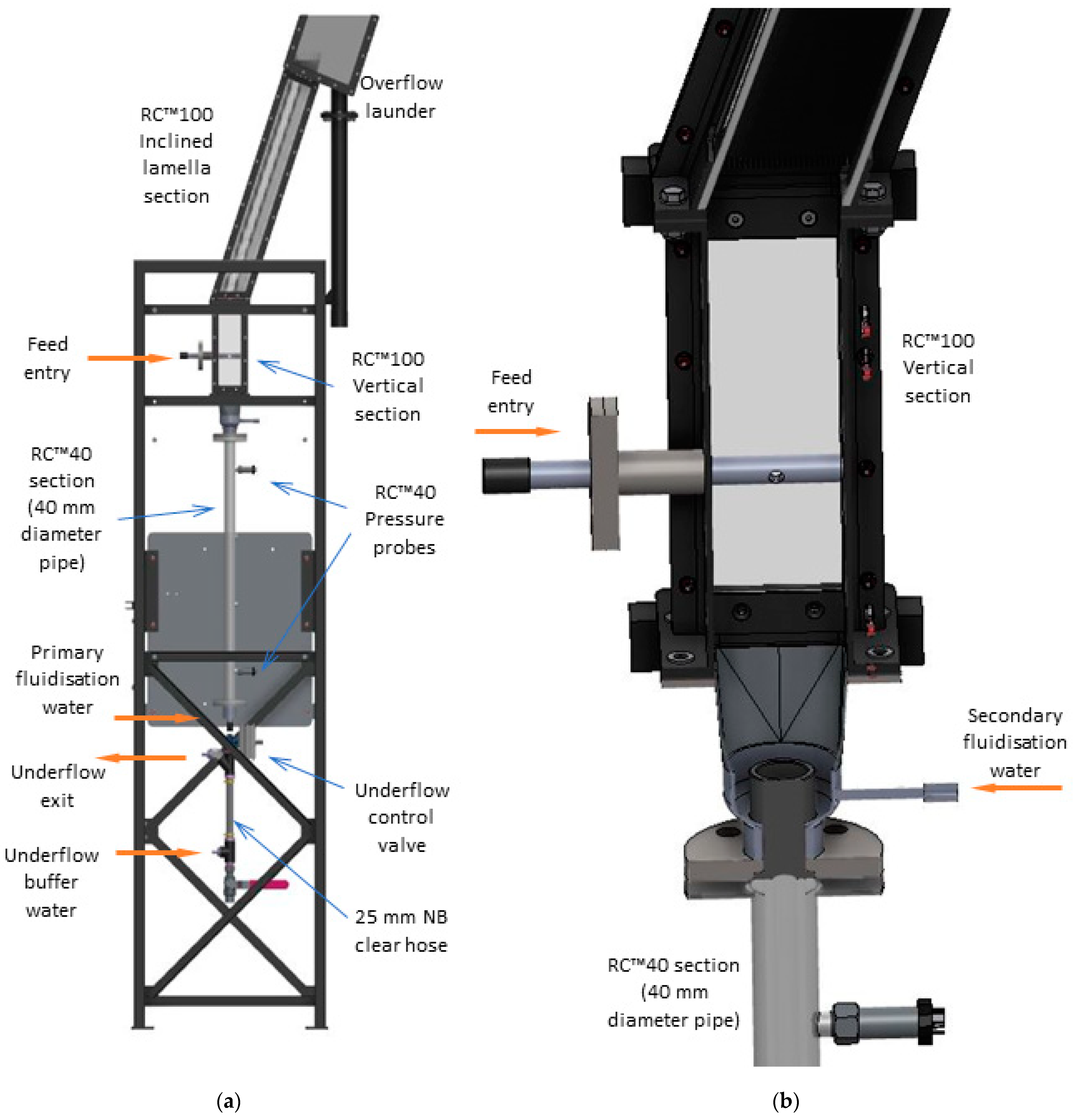
2.2. Continuous Separation Experiment—Source of Primary Separation Samples
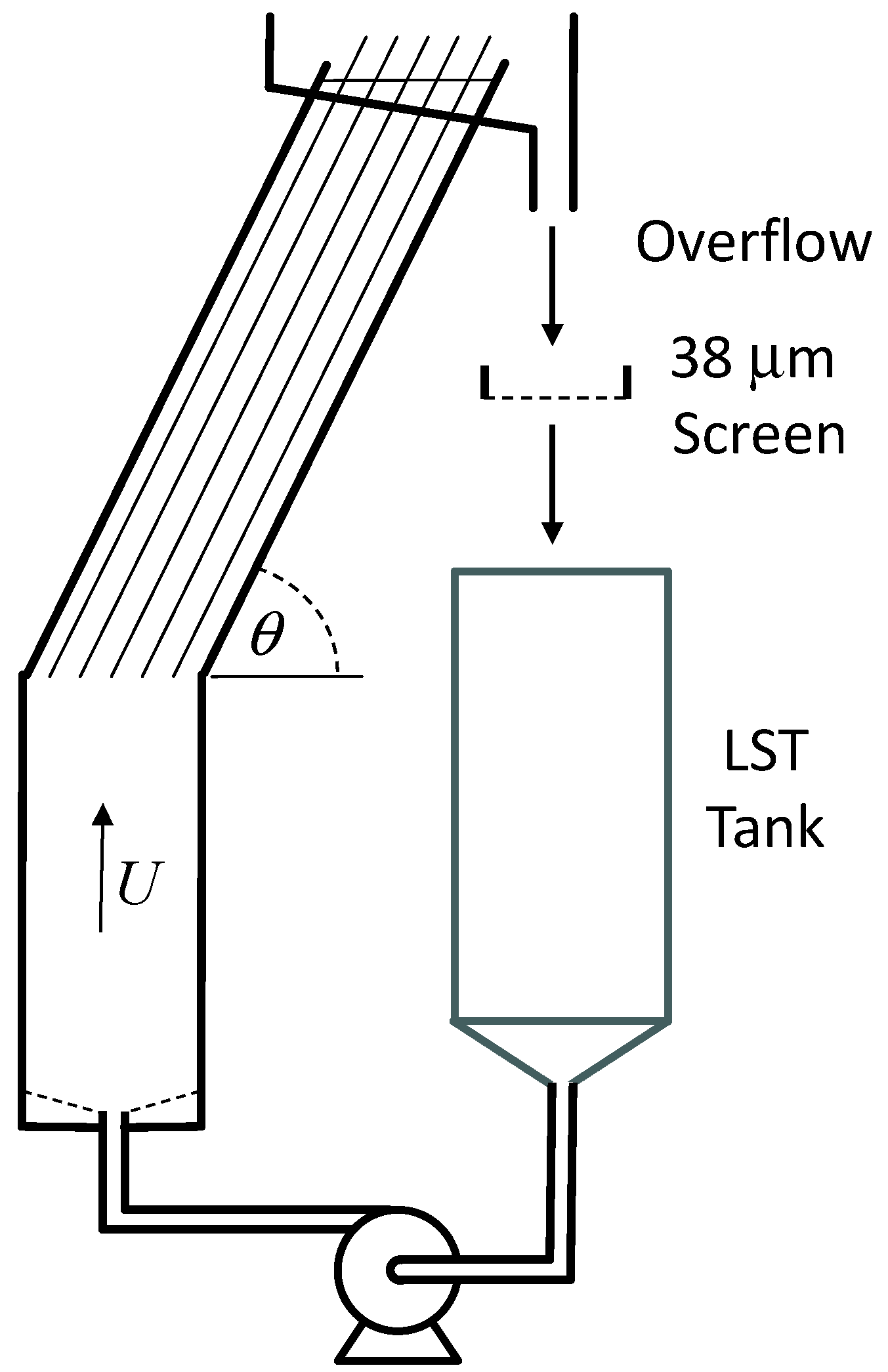
2.3. Batch Fractionation Experiments—Source of Flow Fractionation Samples
2.4. Data Analysis
3. Results and Discussion
3.1. Application of the Algorithm of Galvin et al. [20]
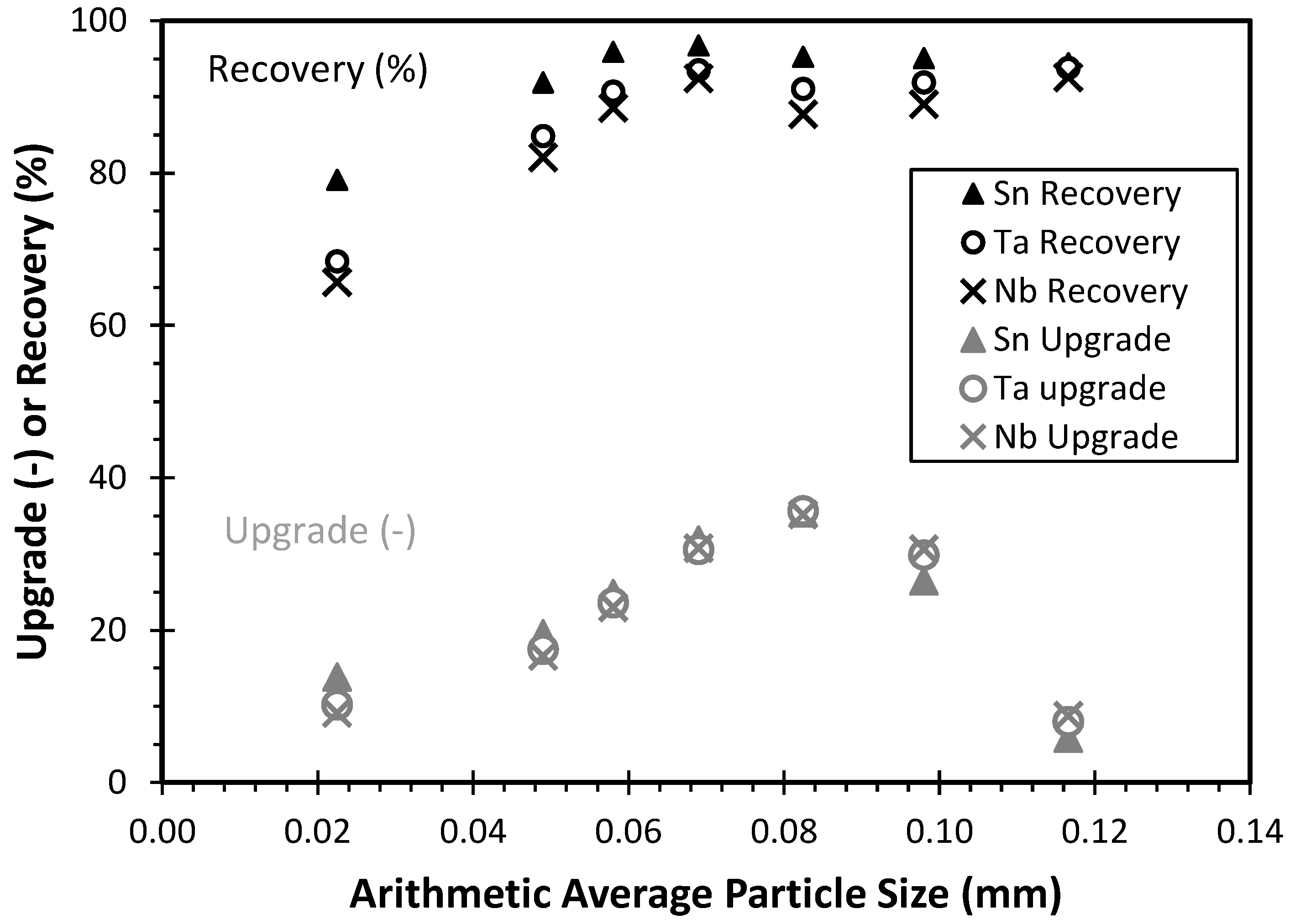
3.2. Approximate Partition Analysis Using the “Tracer Species Recovery” Method
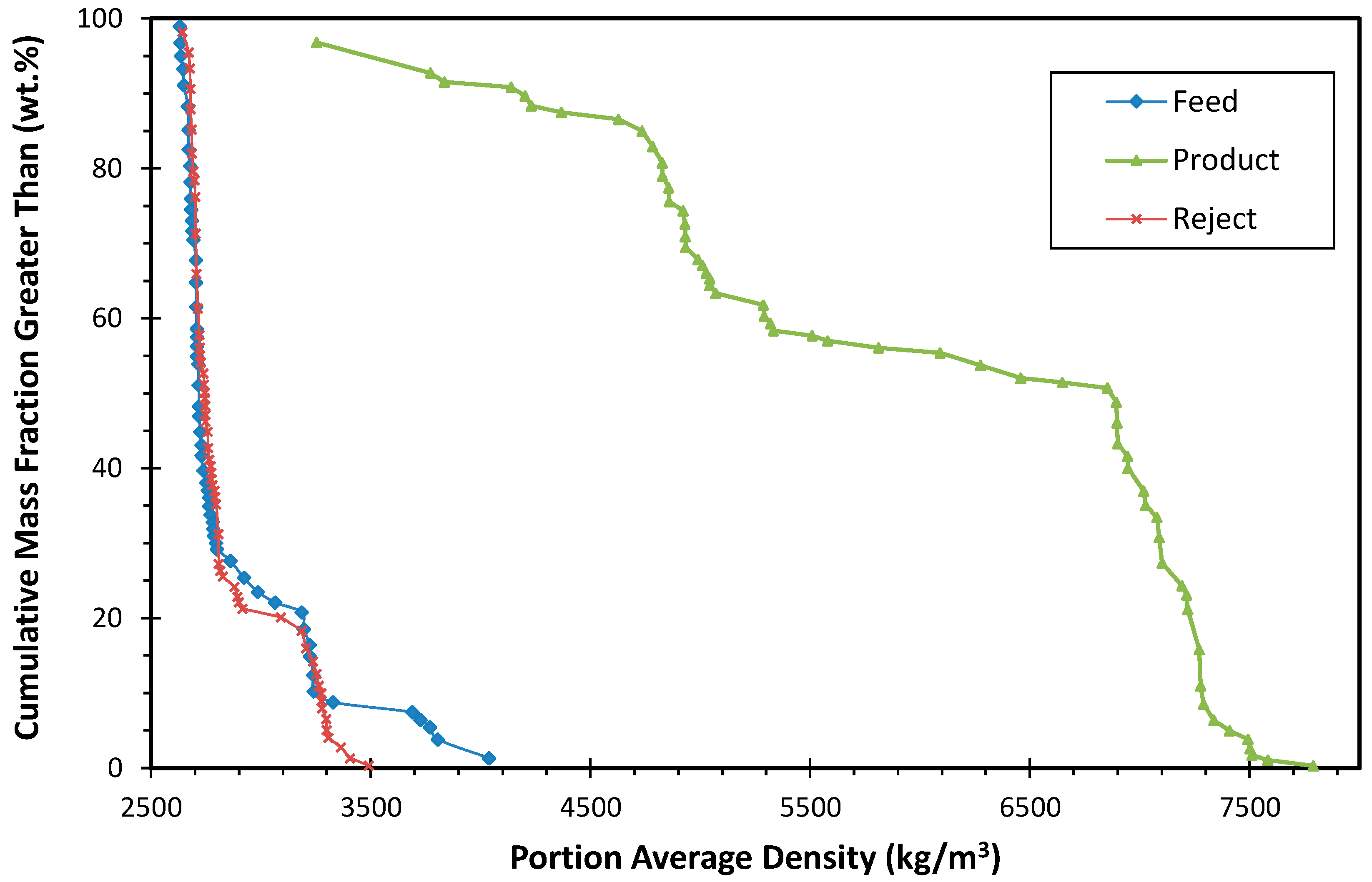
3.3. Partition Curve Estimation Using the “Full Species Distribution” Method
4. Conclusions
Author Contributions
Funding
Data Availability Statement
Conflicts of Interest
Appendix A. Mass-Balanced Assay Data

| Sample | Li2O | Fe2O3 | Al2O3 | SiO2 | TiO2 | Mn | S | P | Sn | Ta2O5 | Nb2O5 | Na2O | PbO | CaO | MgO | K2O | Rb | U3O8 | ThO2 | LOI |
|---|---|---|---|---|---|---|---|---|---|---|---|---|---|---|---|---|---|---|---|---|
| (wt.%) | (wt.%) | (wt.%) | (wt.%) | (wt.%) | (wt.%) | (wt.%) | (wt.%) | (wt.%) | (wt.%) | (wt.%) | (wt.%) | (wt.%) | (wt.%) | (wt.%) | (wt.%) | (wt.%) | (wt.%) | (wt.%) | (wt.%) | |
| Head assay mass balancing relative adjustment (%): | ||||||||||||||||||||
| Feed | 0.4 | −0.7 | 0.3 | −0.2 | 1.0 | −3.3 | −4.0 | 0.1 | 5.7 | 3.1 | −0.2 | 0.6 | −10.4 | −1.3 | 1.5 | −0.7 | −2.2 | 12.3 | −2.2 | −1.9 |
| Product | 0.0 | 0.3 | 0.0 | 0.0 | −0.1 | 1.7 | 3.0 | 0.0 | −4.4 | −2.5 | 0.1 | 0.0 | 11.3 | 0.0 | 0.0 | 0.0 | 0.0 | −6.3 | 0.7 | 0.5 |
| Reject | −0.4 | 0.5 | −0.3 | 0.2 | −0.9 | 2.0 | 1.6 | −0.1 | −0.2 | −0.3 | 0.0 | −0.6 | 4.2 | 1.3 | −1.4 | 0.8 | 2.4 | −2.4 | 1.7 | 1.6 |
| Head assay mass balancing results: | ||||||||||||||||||||
| Feed (wt.%) | 0.831 | 1.867 | 15.178 | 66.123 | 0.106 | 0.114 | 0.776 | 0.802 | 1.369 | 0.579 | 0.199 | 4.064 | 0.013 | 3.278 | 0.507 | 1.425 | 0.092 | 0.008 | 0.002 | 1.265 |
| Product (wt.%) | 0.255 | 16.442 | 1.750 | 4.280 | 0.324 | 1.349 | 12.621 | 0.222 | 33.025 | 12.974 | 4.365 | 0.160 | 0.238 | 1.200 | 0.140 | 0.141 | 0.006 | 0.153 | 0.014 | 7.818 |
| Reject (wt.%) | 0.855 | 1.266 | 15.731 | 68.671 | 0.097 | 0.063 | 0.288 | 0.826 | 0.065 | 0.068 | 0.027 | 4.225 | 0.004 | 3.364 | 0.523 | 1.478 | 0.096 | 0.002 | 0.001 | 0.995 |
| Yield (wt.%) | 4.0 | 4.0 | 4.0 | 4.0 | 4.0 | 4.0 | 4.0 | 4.0 | 4.0 | 4.0 | 4.0 | 4.0 | 4.0 | 4.0 | 4.0 | 4.0 | 4.0 | 4.0 | 4.0 | 4.0 |
| Recovery (%) | 1.2 | 34.9 | 0.5 | 0.3 | 12.1 | 46.8 | 64.4 | 1.1 | 95.5 | 88.7 | 86.9 | 0.2 | 70.2 | 1.4 | 1.1 | 0.4 | 0.3 | 73.7 | 28.3 | 24.5 |
| Upgrade (-) | 0.3 | 8.8 | 0.1 | 0.1 | 3.1 | 11.8 | 16.3 | 0.3 | 24.1 | 22.4 | 22.0 | 0.0 | 17.7 | 0.4 | 0.3 | 0.1 | 0.1 | 18.6 | 7.2 | 6.2 |
| +0.045 mm mass balancing relative adjustments (%): | ||||||||||||||||||||
| Feed | 2.1 | −0.8 | −0.1 | 0.2 | 1.1 | −0.8 | −4.6 | −0.8 | 5.3 | 3.5 | 2.8 | 0.6 | 6.7 | −0.9 | −2.3 | −1.4 | 0.4 | −6.3 | −13.9 | −1.9 |
| Product | 0.0 | 0.4 | 0.0 | 0.0 | −0.1 | 0.4 | 3.7 | 0.0 | −4.2 | −2.9 | −2.2 | 0.0 | −3.7 | 0.0 | 0.0 | 0.0 | 0.0 | 6.4 | 4.8 | 0.6 |
| Reject | −1.9 | 0.5 | 0.1 | −0.2 | −0.9 | 0.4 | 1.7 | 0.9 | −0.2 | −0.3 | −0.3 | −0.6 | −1.8 | 0.9 | 2.5 | 1.4 | −0.4 | 1.6 | 20.9 | 1.4 |
| +0.045 mm mass balancing results: | ||||||||||||||||||||
| Feed (wt.%) | 0.793 | 1.795 | 15.095 | 66.759 | 0.105 | 0.102 | 0.726 | 0.785 | 1.323 | 0.546 | 0.181 | 4.134 | 0.012 | 3.240 | 0.488 | 1.397 | 0.091 | 0.007 | 0.002 | 1.197 |
| Product (wt.%) | 0.327 | 18.224 | 2.110 | 5.280 | 0.338 | 1.210 | 11.966 | 0.266 | 30.829 | 12.130 | 3.927 | 0.190 | 0.193 | 1.350 | 0.170 | 0.153 | 0.006 | 0.140 | 0.012 | 8.702 |
| Reject (wt.%) | 0.813 | 1.085 | 15.656 | 69.416 | 0.095 | 0.054 | 0.240 | 0.808 | 0.048 | 0.045 | 0.019 | 4.305 | 0.004 | 3.321 | 0.502 | 1.450 | 0.095 | 0.002 | 0.002 | 0.872 |
| Yield (wt.%) | 4.1 | 4.1 | 4.1 | 4.1 | 4.1 | 4.1 | 4.1 | 4.1 | 4.1 | 4.1 | 4.1 | 4.1 | 4.1 | 4.1 | 4.1 | 4.1 | 4.1 | 4.1 | 4.1 | 4.1 |
| Recovery (%) | 1.7 | 42.1 | 0.6 | 0.3 | 13.3 | 49.1 | 68.3 | 1.4 | 96.5 | 92.1 | 90.0 | 0.2 | 67.9 | 1.7 | 1.4 | 0.5 | 0.3 | 78.8 | 23.5 | 30.1 |
| Upgrade (-) | 0.4 | 10.2 | 0.1 | 0.1 | 3.2 | 11.8 | 16.5 | 0.3 | 23.3 | 22.2 | 21.7 | 0.0 | 16.4 | 0.4 | 0.3 | 0.1 | 0.1 | 19.0 | 5.7 | 7.3 |
| −0.045 mm bass balancing relative adjustments (%): | ||||||||||||||||||||
| Feed | 3.5 | −0.2 | 3.2 | −1.3 | 2.1 | −2.7 | −11.4 | 3.1 | 2.4 | −4.5 | −6.6 | −2.3 | 7.1 | 1.5 | 9.4 | 9.8 | 5.7 | 11.5 | 12.2 | 3.2 |
| Product | 0.0 | 0.0 | 0.0 | 0.0 | −0.2 | 1.1 | 2.1 | 0.0 | −1.7 | 3.5 | 5.1 | 0.0 | −2.5 | 0.0 | 0.0 | 0.0 | 0.0 | −4.8 | −2.6 | −0.1 |
| Reject | −3.0 | 0.2 | −2.8 | 1.4 | −1.8 | 1.8 | 17.2 | −2.7 | −0.5 | 1.7 | 3.1 | 2.5 | −3.3 | −1.4 | −6.8 | −7.0 | −4.6 | −3.7 | −6.1 | −2.7 |
| −0.045 mm mass balancing results: | ||||||||||||||||||||
| Feed (wt.%) | 0.803 | 3.772 | 15.603 | 56.904 | 0.193 | 0.303 | 0.807 | 1.018 | 3.744 | 1.713 | 0.546 | 3.655 | 0.052 | 4.162 | 0.799 | 1.536 | 0.087 | 0.034 | 0.005 | 1.764 |
| Product (wt.%) | 0.014 | 4.631 | 0.310 | 1.210 | 0.260 | 1.966 | 1.848 | 0.023 | 49.813 | 18.904 | 5.613 | 0.050 | 0.375 | 0.470 | 0.030 | 0.080 | 0.003 | 0.325 | 0.024 | 1.358 |
| Reject (wt.%) | 0.853 | 3.717 | 16.577 | 60.454 | 0.189 | 0.197 | 0.741 | 1.082 | 0.808 | 0.617 | 0.223 | 3.885 | 0.032 | 4.397 | 0.848 | 1.629 | 0.092 | 0.016 | 0.004 | 1.790 |
| Yield (wt.%) | 6.0 | 6.0 | 6.0 | 6.0 | 6.0 | 6.0 | 6.0 | 6.0 | 6.0 | 6.0 | 6.0 | 6.0 | 6.0 | 6.0 | 6.0 | 6.0 | 6.0 | 6.0 | 6.0 | 6.0 |
| Recovery (%) | 0.1 | 7.4 | 0.1 | 0.1 | 8.1 | 38.9 | 13.7 | 0.1 | 79.7 | 66.1 | 61.6 | 0.1 | 42.8 | 0.7 | 0.2 | 0.3 | 0.2 | 56.8 | 28.4 | 4.6 |
| Upgrade (-) | 0.0 | 1.2 | 0.0 | 0.0 | 1.3 | 6.5 | 2.3 | 0.0 | 13.3 | 11.0 | 10.3 | 0.0 | 7.2 | 0.1 | 0.0 | 0.1 | 0.0 | 9.5 | 4.7 | 0.8 |
Appendix B. Size × Flow Assay and Density Raw Data
| Sample | Flow Fraction | Mass Fraction | Density | Li2O | Fe2O3 | Al2O3 | SiO2 | TiO2 | Mn | S | P | Sn | Ta2O5 | Nb2O5 | Na2O | PbO | CaO | MgO | K2O | Rb | U3O8 | ThO2 | LOI |
|---|---|---|---|---|---|---|---|---|---|---|---|---|---|---|---|---|---|---|---|---|---|---|---|
| (wt.%) | (RD) | (wt.%) | (wt.%) | (wt.%) | (wt.%) | (wt.%) | (wt.%) | (wt.%) | (wt.%) | (wt.%) | (wt.%) | (wt.%) | (wt.%) | (wt.%) | (wt.%) | (wt.%) | (wt.%) | (wt.%) | (wt.%) | (wt.%) | (wt.%) | ||
| Feed | Flow 1 | 6.79 | 2.680 | 0.063 | 0.230 | 17.630 | 67.560 | 0.018 | 0.009 | 0.032 | 0.111 | 0.080 | 0.022 | 0.009 | 4.180 | 0.006 | 0.320 | 0.160 | 7.802 | 0.5326 | 0.0021 | 0.0004 | 0.61 |
| Flow 2 | 7.59 | 2.701 | 0.028 | 0.160 | 16.970 | 71.510 | 0.015 | 0.006 | 0.005 | 0.063 | 0.017 | 0.005 | 0.003 | 7.820 | 0.002 | 0.360 | 0.130 | 2.264 | 0.1345 | 0.0007 | 0.0003 | 0.41 | |
| Flow 3 | 10.96 | 2.692 | 0.019 | 0.130 | 15.470 | 74.790 | 0.014 | 0.004 | 0.003 | 0.047 | 0.010 | 0.002 | 0.001 | 8.160 | 0.002 | 0.460 | 0.090 | 0.555 | 0.0195 | 0.0003 | 0.0002 | 0.30 | |
| Flow 4 | 8.59 | 2.679 | 0.028 | 0.140 | 14.290 | 76.630 | 0.017 | 0.004 | 0.002 | 0.041 | 0.008 | 0.002 | 0.001 | 7.260 | 0.002 | 0.580 | 0.090 | 0.565 | 0.0213 | 0.0004 | 0.0001 | 0.27 | |
| Flow 5 | 5.92 | 2.672 | 0.031 | 0.190 | 11.790 | 80.650 | 0.021 | 0.004 | 0.003 | 0.033 | 0.006 | 0.002 | 0.001 | 5.460 | 0.001 | 0.930 | 0.100 | 0.403 | 0.0112 | 0.0003 | 0.0001 | 0.32 | |
| Flow 6 | 10.94 | 2.703 | 0.038 | 0.280 | 11.020 | 81.800 | 0.028 | 0.007 | 0.019 | 0.033 | 0.048 | 0.018 | 0.006 | 4.430 | 0.001 | 1.360 | 0.130 | 0.426 | 0.0122 | 0.0004 | 0.0002 | 0.35 | |
| Flow 7 | 10.55 | 2.703 | 0.042 | 0.260 | 10.080 | 83.290 | 0.030 | 0.007 | 0.005 | 0.029 | 0.011 | 0.003 | 0.000 | 3.860 | 0.000 | 1.350 | 0.130 | 0.432 | 0.0128 | 0.0003 | 0.0002 | 0.37 | |
| Flow 8 | 9.59 | 2.733 | 0.085 | 0.500 | 11.590 | 80.220 | 0.055 | 0.011 | 0.008 | 0.041 | 0.024 | 0.006 | 0.003 | 3.180 | 0.001 | 2.030 | 0.270 | 0.835 | 0.0371 | 0.0003 | 0.0003 | 0.62 | |
| Flow 9 | 7.38 | 2.910 | 1.721 | 1.800 | 23.240 | 60.360 | 0.170 | 0.067 | 0.017 | 0.421 | 0.041 | 0.010 | 0.005 | 1.680 | 0.004 | 2.200 | 0.970 | 3.794 | 0.3138 | 0.0006 | 0.0006 | 2.13 | |
| Flow 10 | 11.91 | 3.207 | 3.901 | 3.860 | 22.690 | 44.980 | 0.309 | 0.156 | 1.210 | 3.191 | 0.106 | 0.136 | 0.050 | 0.680 | 0.004 | 10.030 | 1.490 | 0.912 | 0.0666 | 0.0043 | 0.0039 | 1.95 | |
| Flow 11 | 9.79 | 3.942 | 1.871 | 10.270 | 12.080 | 24.470 | 0.385 | 0.609 | 6.040 | 3.201 | 12.338 | 5.148 | 1.677 | 0.540 | 0.055 | 10.260 | 0.990 | 0.296 | 0.0167 | 0.0600 | 0.0090 | 3.72 | |
| Underflow Product | Flow 1 | 10.17 | 3.550 | 2.915 | 11.630 | 16.260 | 35.400 | 0.495 | 0.214 | 9.428 | 2.272 | 0.365 | 0.484 | 0.206 | 0.750 | 0.037 | 7.230 | 1.120 | 0.397 | 0.0237 | 0.0307 | 0.0174 | 6.52 |
| Flow 2 | 8.00 | 4.760 | 0.355 | 42.060 | 2.680 | 7.640 | 0.642 | 0.172 | 28.854 | 0.256 | 1.002 | 1.942 | 0.825 | 0.460 | 0.078 | 1.060 | 0.320 | 0.215 | 0.0070 | 0.0538 | 0.0124 | 23.19 | |
| Flow 3 | 8.99 | 4.940 | 0.143 | 46.330 | 1.470 | 4.440 | 0.490 | 0.297 | 28.815 | 0.094 | 2.245 | 4.017 | 1.789 | 0.370 | 0.093 | 0.780 | 0.230 | 0.207 | 0.0073 | 0.0702 | 0.0088 | 24.85 | |
| Flow 4 | 10.12 | 5.455 | 0.026 | 40.090 | 0.830 | 2.800 | 0.334 | 1.023 | 25.980 | 0.058 | 9.859 | 10.782 | 5.127 | 0.320 | 0.159 | 1.100 | 0.130 | 0.186 | 0.0059 | 0.1076 | 0.0094 | 19.92 | |
| Flow 5 | 9.62 | 5.983 | 0.016 | 26.560 | 0.610 | 1.910 | 0.302 | 1.726 | 17.190 | 0.038 | 23.412 | 15.884 | 7.086 | 0.260 | 0.189 | 1.070 | 0.070 | 0.168 | 0.0056 | 0.1139 | 0.0087 | 12.35 | |
| Flow 6 | 8.32 | 6.707 | 0.003 | 13.350 | 0.480 | 1.440 | 0.303 | 2.025 | 8.717 | 0.026 | 38.288 | 18.256 | 7.320 | 0.200 | 0.216 | 0.910 | 0.030 | 0.136 | 0.0041 | 0.1140 | 0.0081 | 5.70 | |
| Flow 7 | 7.11 | 7.143 | 0.009 | 8.220 | 0.430 | 1.270 | 0.304 | 2.019 | 4.808 | 0.023 | 44.877 | 18.359 | 6.813 | 0.180 | 0.229 | 0.810 | 0.020 | 0.121 | 0.0036 | 0.1166 | 0.0081 | 3.20 | |
| Flow 8 | 6.56 | 7.759 | 0.000 | 2.870 | 0.340 | 0.900 | 0.284 | 1.933 | 0.642 | 0.015 | 53.340 | 17.619 | 5.788 | 0.130 | 0.236 | 0.550 | 0.000 | 0.095 | 0.0026 | 0.1077 | 0.0073 | 0.57 | |
| Flow 9 | 14.45 | 7.340 | 0.014 | 3.400 | 0.450 | 1.410 | 0.271 | 1.661 | 1.088 | 0.024 | 55.020 | 15.614 | 4.508 | 0.150 | 0.220 | 0.440 | 0.010 | 0.088 | 0.0023 | 0.1074 | 0.0073 | 0.86 | |
| Flow 10 | 8.57 | 7.819 | 0.005 | 2.040 | 0.320 | 1.080 | 0.260 | 1.379 | 0.192 | 0.015 | 60.004 | 13.986 | 3.018 | 0.120 | 0.244 | 0.240 | 0.000 | 0.062 | 0.0021 | 0.1469 | 0.0097 | 0.29 | |
| Flow 11 | 8.09 | 7.646 | 0.015 | 2.340 | 0.290 | 0.890 | 0.259 | 1.361 | 0.443 | 0.017 | 59.653 | 14.337 | 2.605 | 0.100 | 0.290 | 0.220 | 0.000 | 0.057 | 0.0022 | 0.3956 | 0.0266 | 0.43 | |
| Overflow Tailings Reject | Flow 1 | 9.80 | 2.650 | 0.047 | 0.160 | 17.390 | 68.780 | 0.013 | 0.008 | 0.008 | 0.096 | 0.012 | 0 | 0 | 5.440 | 0.005 | 0.310 | 0.110 | 6.236 | 0.4419 | 0.0005 | 0.0002 | 0.38 |
| Flow 2 | 8.60 | 2.679 | 0.024 | 0.150 | 15.240 | 74.510 | 0.014 | 0.007 | 0.003 | 0.051 | 0.016 | 0.007 | 0.003 | 7.670 | 0.004 | 0.480 | 0.080 | 0.997 | 0.0530 | 0.0003 | 0.0001 | 0.24 | |
| Flow 3 | 9.63 | 2.701 | 0.032 | 0.180 | 13.760 | 77.290 | 0.023 | 0.005 | 0.003 | 0.044 | 0.014 | 0.004 | 0.000 | 6.690 | 0.003 | 0.710 | 0.100 | 0.778 | 0.0344 | 0.0002 | 0.0001 | 0.28 | |
| Flow 4 | 10.96 | 2.710 | 0.029 | 0.210 | 12.750 | 79.200 | 0.021 | 0.006 | 0.002 | 0.035 | 0.004 | 0.001 | 0 | 5.900 | 0.004 | 1.020 | 0.110 | 0.479 | 0.0162 | 0.0002 | 0.0001 | 0.20 | |
| Flow 5 | 5.49 | 2.705 | 0.028 | 0.230 | 11.760 | 80.340 | 0.027 | 0.005 | 0.002 | 0.033 | 0.004 | 0 | 0 | 5.120 | 0.003 | 1.170 | 0.120 | 0.443 | 0.0140 | 0.0001 | 0.0002 | 0.25 | |
| Flow 6 | 11.29 | 2.707 | 0.033 | 0.220 | 11.900 | 80.270 | 0.022 | 0.005 | 0.002 | 0.035 | 0.005 | 0.001 | 0 | 5.380 | 0.004 | 1.050 | 0.110 | 0.443 | 0.0141 | 0.0002 | 0.0001 | 0.26 | |
| Flow 7 | 9.79 | 2.708 | 0.058 | 0.350 | 11.610 | 80.880 | 0.040 | 0.009 | 0.004 | 0.038 | 0.008 | 0 | 0 | 4.100 | 0.003 | 1.590 | 0.180 | 0.634 | 0.0274 | 0.0002 | 0.0002 | 0.39 | |
| Flow 8 | 13.51 | 2.806 | 0.839 | 1.020 | 16.620 | 72.290 | 0.098 | 0.033 | 0.010 | 0.150 | 0.018 | 0.006 | 0.003 | 2.800 | 0.004 | 1.730 | 0.550 | 2.035 | 0.1617 | 0.0004 | 0.0004 | 1.10 | |
| Flow 9 | 4.57 | 3.129 | 4.314 | 2.110 | 26.260 | 53.960 | 0.194 | 0.097 | 0.020 | 1.242 | 0.038 | 0.007 | 0.003 | 0.740 | 0.002 | 4.090 | 1.290 | 1.798 | 0.1451 | 0.0007 | 0.0009 | 1.54 | |
| Flow 10 | 8.80 | 3.121 | 3.635 | 3.390 | 22.100 | 42.730 | 0.311 | 0.174 | 0.648 | 3.854 | 0.082 | 0.093 | 0.034 | 0.720 | 0.005 | 12.080 | 1.610 | 0.694 | 0.0530 | 0.0035 | 0.0042 | 1.61 | |
| Flow 11 | 7.55 | 3.306 | 2.901 | 5.890 | 17.810 | 36.930 | 0.401 | 0.230 | 2.455 | 4.706 | 0.671 | 0.569 | 0.205 | 0.830 | 0.012 | 14.680 | 1.400 | 0.403 | 0.0252 | 0.0094 | 0.0071 | 2.47 |
| Sample | Size Interval | Mass Fraction | Density | Li2O | Fe2O3 | Al2O3 | SiO2 | TiO2 | Mn | S | P | Sn | Ta2O5 | Nb2O5 | Na2O | PbO | CaO | MgO | K2O | Rb | U3O8 | ThO2 | LOI |
|---|---|---|---|---|---|---|---|---|---|---|---|---|---|---|---|---|---|---|---|---|---|---|---|
| (wt.%) | (RD) | (wt.%) | (wt.%) | (wt.%) | (wt.%) | (wt.%) | (wt.%) | (wt.%) | (wt.%) | (wt.%) | (wt.%) | (wt.%) | (wt.%) | (wt.%) | (wt.%) | (wt.%) | (wt.%) | (wt.%) | (wt.%) | (wt.%) | (wt.%) | ||
| Feed Flow 1 | 1 | 6.2 | |||||||||||||||||||||
| 2 | 10.6 | 2.6359 | 0.05 | 0.23 | 17.67 | 67.11 | 0.028 | 0.009 | 0.022 | 0.113 | 0.037 | 0.009 | 0.003 | 3.95 | 0.004 | 0.21 | 0.13 | 8.58 | 0.572 | 0.0006 | 0.0001 | 0.84 | |
| 3 | 10.5 | 2.7095 | 0.04 | 0.21 | 17.63 | 67.78 | 0.002 | 0.008 | 0.019 | 0.11 | 0.035 | 0.008 | 0 | 4.05 | 0.004 | 0.24 | 0.14 | 8.23 | 0.582 | 0.0003 | 0.0001 | 0.62 | |
| 4 | 29.7 | 2.6323 | 0.04 | 0.21 | 17.53 | 67.82 | 0.004 | 0.008 | 0.024 | 0.106 | 0.05 | 0.017 | 0.004 | 4.23 | 0.002 | 0.31 | 0.15 | 7.81 | 0.535 | 0.0004 | 0.0001 | 0.60 | |
| 5 | 25.0 | 2.6507 | 0.06 | 0.23 | 17.74 | 67.90 | 0.007 | 0.01 | 0.033 | 0.108 | 0.082 | 0.03 | 0.009 | 4.33 | 0.004 | 0.37 | 0.16 | 7.50 | 0.511 | 0.0006 | 0.0002 | 0.63 | |
| 6 | 15.3 | 2.7150 | 0.06 | 0.30 | 17.74 | 67.53 | 0.017 | 0.014 | 0.04 | 0.11 | 0.133 | 0.052 | 0.016 | 4.46 | 0.004 | 0.42 | 0.18 | 7.22 | 0.486 | 0.0011 | 0.0002 | 0.83 | |
| 7 | 2.6 | ||||||||||||||||||||||
| Feed Flow 2 | 1 | 1.6 | |||||||||||||||||||||
| 2 | 3.9 | ||||||||||||||||||||||
| 3 | 6.1 | 2.6885 | 0.03 | 0.20 | 18.60 | 67.86 | 0.007 | 0.005 | 0.005 | 0.08 | 0.011 | 0.001 | 0 | 8.05 | 0 | 0.16 | 0.15 | 3.59 | 0.215 | 0.0003 | 0.0001 | 0.66 | |
| 4 | 29.7 | 2.6346 | 0.02 | 0.14 | 17.21 | 71.01 | 0.003 | 0.005 | 0.003 | 0.064 | 0.009 | 0.001 | 0 | 8.08 | 0 | 0.25 | 0.12 | 2.35 | 0.137 | 0.0002 | 0.0000 | 0.47 | |
| 5 | 31.3 | 2.6466 | 0.02 | 0.16 | 16.62 | 71.72 | 0.009 | 0.004 | 0.003 | 0.056 | 0.006 | 0.002 | 0 | 7.77 | 0 | 0.39 | 0.12 | 2.07 | 0.115 | 0.0002 | 0.0001 | 0.41 | |
| 6 | 23.3 | 2.6860 | 0.02 | 0.18 | 16.49 | 72.35 | 0.007 | 0.005 | 0.004 | 0.055 | 0.014 | 0.005 | 0 | 7.61 | 0 | 0.52 | 0.13 | 1.87 | 0.106 | 0.0002 | 0.0001 | 0.53 | |
| 7 | 4.1 | ||||||||||||||||||||||
| Feed Flow 3 | 1 | 4.2 | |||||||||||||||||||||
| 2 | 8.9 | 2.6783 | 0.02 | 0.10 | 17.16 | 71.75 | 0 | 0.003 | 0.002 | 0.061 | 0.002 | 0.002 | 0 | 9.57 | 0 | 0.13 | 0.07 | 0.59 | 0.020 | 0.0002 | 0.0001 | 0.36 | |
| 3 | 9.7 | 2.6842 | 0.02 | 0.10 | 16.20 | 73.40 | 0 | 0.003 | 0.002 | 0.055 | 0.002 | 0 | 0 | 8.86 | 0 | 0.19 | 0.08 | 0.55 | 0.019 | 0.0002 | 0.0001 | 0.28 | |
| 4 | 34.5 | 2.6677 | 0.02 | 0.12 | 15.23 | 75.11 | 0.005 | 0.003 | 0.002 | 0.046 | 0.002 | 0.002 | 0 | 8.11 | 0 | 0.41 | 0.08 | 0.52 | 0.017 | 0.0002 | 0.0001 | 0.25 | |
| 5 | 24.9 | 2.6724 | 0.02 | 0.14 | 15.07 | 75.27 | 0.007 | 0.003 | 0.002 | 0.042 | 0.004 | 0.001 | 0 | 7.76 | 0 | 0.60 | 0.09 | 0.56 | 0.018 | 0.0002 | 0.0001 | 0.31 | |
| 6 | 15.3 | 2.6821 | 0.02 | 0.18 | 15.04 | 75.31 | 0.036 | 0.005 | 0.003 | 0.041 | 0.007 | 0.004 | 0 | 7.46 | 0.001 | 0.75 | 0.10 | 0.60 | 0.021 | 0.0002 | 0.0001 | 0.29 | |
| 7 | 2.6 | ||||||||||||||||||||||
| Feed Flow 4 | 1 | 3.6 | |||||||||||||||||||||
| 2 | 7.2 | 2.7104 | 0.012 | 0.11 | 16.06 | 73.40 | 0.011 | 0.003 | 0.002 | 0.057 | 0.002 | 0.003 | 0 | 8.82 | 0 | 0.17 | 0.08 | 0.69 | 0.028 | 0.0002 | 0 | 0.43 | |
| 3 | 9.1 | 2.7293 | 0.017 | 0.11 | 15.04 | 75.22 | 0.003 | 0.004 | 0.002 | 0.049 | 0.002 | 0.002 | 0 | 8.05 | 0 | 0.26 | 0.08 | 0.609 | 0.025 | 0.0002 | 0.0001 | 0.44 | |
| 4 | 32.5 | 2.6806 | 0.014 | 0.13 | 14.14 | 76.83 | 0.005 | 0.003 | 0.003 | 0.043 | 0.001 | 0 | 0 | 7.31 | 0 | 0.50 | 0.08 | 0.536 | 0.019 | 0.0001 | 0.0001 | 0.26 | |
| 5 | 28.4 | 2.6713 | 0.014 | 0.15 | 13.88 | 77.26 | 0.008 | 0.003 | 0.002 | 0.038 | 0.003 | 0 | 0 | 6.89 | 0 | 0.71 | 0.09 | 0.539 | 0.018 | 0.0002 | 0.0001 | 0.24 | |
| 6 | 16.9 | 2.6932 | 0.024 | 0.22 | 13.87 | 77.27 | 0.014 | 0.004 | 0.003 | 0.035 | 0.004 | 0.001 | 0 | 6.53 | 0 | 0.91 | 0.11 | 0.571 | 0.018 | 0.0002 | 0.0002 | 0.34 | |
| 7 | 2.4 | ||||||||||||||||||||||
| Feed Flow 5 | 1 | 3.9 | |||||||||||||||||||||
| 2 | 7.8 | ||||||||||||||||||||||
| 3 | 9.0 | 2.7654 | 0.022 | 0.16 | 11.53 | 80.85 | 0.009 | 0.003 | 0.003 | 0.039 | 0.003 | 0.002 | 0.000 | 5.93 | 0 | 0.40 | 0.09 | 0.41 | 0.012 | 0.0002 | 0.0001 | 0.31 | |
| 4 | 34.4 | 2.7050 | 0.029 | 0.19 | 11.38 | 81.38 | 0.013 | 0.003 | 0.003 | 0.032 | 0.001 | 0.002 | 0.000 | 5.28 | 0 | 0.92 | 0.10 | 0.39 | 0.010 | 0.0002 | 0.0002 | 0.24 | |
| 5 | 28.5 | 2.7099 | 0.017 | 0.20 | 11.94 | 80.23 | 0.014 | 0.004 | 0.002 | 0.031 | 0.004 | 0.002 | 0.000 | 5.34 | 0 | 1.14 | 0.11 | 0.41 | 0.010 | 0.0002 | 0.0002 | 0.31 | |
| 6 | 14.9 | 2.7821 | 0.023 | 0.23 | 12.61 | 79.25 | 0.016 | 0.005 | 0.003 | 0.03 | 0.006 | 0.003 | 0.000 | 5.43 | 0 | 1.31 | 0.11 | 0.45 | 0.011 | 0.0002 | 0.0002 | 0.38 | |
| 7 | 1.5 | ||||||||||||||||||||||
| Feed Flow 6 | 1 | 4.9 | |||||||||||||||||||||
| 2 | 8.6 | 2.7086 | 0.025 | 0.24 | 9.98 | 83.17 | 0.013 | 0.004 | 0.024 | 0.039 | 0.019 | 0.008 | 0.003 | 4.88 | 0 | 0.49 | 0.11 | 0.39 | 0.011 | 0.0003 | 0.0001 | 0.29 | |
| 3 | 9.0 | 2.7644 | 0.033 | 0.27 | 10.2 | 83.07 | 0.019 | 0.006 | 0.016 | 0.038 | 0.028 | 0.009 | 0.000 | 4.47 | 0 | 0.87 | 0.13 | 0.43 | 0.012 | 0.0002 | 0.0002 | 0.27 | |
| 4 | 38.7 | 2.7065 | 0.027 | 0.27 | 10.72 | 82.18 | 0.022 | 0.006 | 0.014 | 0.031 | 0.028 | 0.013 | 0.003 | 4.28 | 0 | 1.38 | 0.12 | 0.41 | 0.011 | 0.0002 | 0.0002 | 0.31 | |
| 5 | 24.9 | 2.7245 | 0.026 | 0.29 | 11.54 | 80.73 | 0.023 | 0.007 | 0.025 | 0.03 | 0.062 | 0.023 | 0.005 | 4.35 | 0 | 1.69 | 0.13 | 0.44 | 0.012 | 0.0004 | 0.0002 | 0.37 | |
| 6 | 12.5 | 2.7192 | 0.035 | 0.35 | 12.37 | 79.38 | 0.026 | 0.01 | 0.035 | 0.033 | 0.13 | 0.054 | 0.013 | 4.52 | 0.001 | 1.91 | 0.15 | 0.50 | 0.015 | 0.0008 | 0.0003 | 0.41 | |
| 7 | 1.5 | ||||||||||||||||||||||
| Feed Flow 7 | 1 | 7.5 | |||||||||||||||||||||
| 2 | 10.8 | 2.7515 | 0.033 | 0.21 | 9.31 | 84.6 | 0.015 | 0.004 | 0.006 | 0.035 | 0.004 | 0.003 | 0.000 | 4.25 | 0 | 0.55 | 0.12 | 0.42 | 0.012 | 0.0002 | 0.0002 | 0.30 | |
| 3 | 8.7 | 2.7593 | 0.035 | 0.24 | 9.05 | 84.94 | 0.018 | 0.005 | 0.005 | 0.032 | 0.006 | 0.004 | 0.001 | 3.80 | 0 | 0.82 | 0.13 | 0.44 | 0.013 | 0.0002 | 0.0002 | 0.33 | |
| 4 | 42.2 | 2.7172 | 0.026 | 0.26 | 9.72 | 84.06 | 0.021 | 0.006 | 0.004 | 0.026 | 0.005 | 0.004 | 0.000 | 3.58 | 0 | 1.44 | 0.13 | 0.41 | 0.011 | 0.0001 | 0.0002 | 0.24 | |
| 5 | 18.7 | 2.7388 | 0.03 | 0.28 | 10.82 | 82.08 | 0.023 | 0.005 | 0.006 | 0.026 | 0.01 | 0.003 | 0.000 | 3.77 | 0.002 | 1.86 | 0.13 | 0.43 | 0.012 | 0.0001 | 0.0003 | 0.28 | |
| 6 | 10.7 | 2.7183 | 0.04 | 0.34 | 11.93 | 79.99 | 0.028 | 0.006 | 0.01 | 0.03 | 0.013 | 0.008 | 0.002 | 4.03 | 0.002 | 2.13 | 0.15 | 0.52 | 0.016 | 0.0002 | 0.0003 | 0.41 | |
| 7 | 1.5 | ||||||||||||||||||||||
| Feed Flow 8 | 1 | 8.7 | |||||||||||||||||||||
| 2 | 10.6 | 2.7720 | 0.068 | 0.52 | 8.43 | 85.50 | 0.045 | 0.01 | 0.007 | 0.046 | 0.011 | 0.005 | 0.002 | 2.35 | 0 | 1.14 | 0.29 | 0.777 | 0.032 | 0.0002 | 0.0003 | 0.58 | |
| 3 | 10.0 | 2.7867 | 0.086 | 0.53 | 9.83 | 83.43 | 0.048 | 0.01 | 0.008 | 0.046 | 0.012 | 0.006 | 0.000 | 2.6 | 0 | 1.51 | 0.30 | 0.877 | 0.038 | 0.0005 | 0.0004 | 0.62 | |
| 4 | 40.3 | 2.7049 | 0.073 | 0.47 | 11.93 | 80.15 | 0.045 | 0.01 | 0.006 | 0.037 | 0.017 | 0.007 | 0.002 | 3.29 | 0 | 2.24 | 0.24 | 0.772 | 0.033 | 0.0003 | 0.0003 | 0.49 | |
| 5 | 19.9 | 2.7297 | 0.061 | 0.47 | 13.49 | 77.54 | 0.046 | 0.011 | 0.010 | 0.035 | 0.028 | 0.011 | 0.004 | 3.76 | 0.002 | 2.64 | 0.24 | 0.801 | 0.034 | 0.0003 | 0.0003 | 0.58 | |
| 6 | 9.4 | 2.7839 | 0.106 | 0.61 | 15.14 | 74.42 | 0.055 | 0.015 | 0.016 | 0.041 | 0.06 | 0.022 | 0.007 | 3.95 | 0.001 | 2.85 | 0.31 | 1.070 | 0.053 | 0.0005 | 0.0004 | 0.74 | |
| 7 | 1.1 | ||||||||||||||||||||||
| Feed Flow 9 | 1 | 10.9 | |||||||||||||||||||||
| 2 | 10.0 | ||||||||||||||||||||||
| 3 | 9.8 | 2.8624 | 0.818 | 1.57 | 22.74 | 62.65 | 0.123 | 0.052 | 0.016 | 0.17 | 0.041 | 0.015 | 0.006 | 1.45 | 0.001 | 1.12 | 0.70 | 4.885 | 0.438 | 0.0005 | 0.0005 | 2.67 | |
| 4 | 28.2 | 2.9233 | 1.664 | 1.81 | 23.82 | 60.1 | 0.174 | 0.064 | 0.015 | 0.319 | 0.038 | 0.01 | 0.003 | 1.77 | 0.001 | 1.99 | 0.97 | 3.937 | 0.315 | 0.0005 | 0.0005 | 2.15 | |
| 5 | 22.0 | 2.9878 | 2.211 | 1.97 | 24.05 | 58.31 | 0.189 | 0.072 | 0.016 | 0.584 | 0.038 | 0.009 | 0.002 | 1.74 | 0 | 2.82 | 1.11 | 3.322 | 0.256 | 0.0006 | 0.0006 | 2.00 | |
| 6 | 15.6 | 3.0662 | 3.286 | 2.13 | 24.87 | 56 | 0.197 | 0.088 | 0.022 | 0.918 | 0.04 | 0.013 | 0.004 | 1.26 | 0.002 | 3.55 | 1.22 | 2.740 | 0.199 | 0.0007 | 0.0009 | 1.96 | |
| 7 | 3.6 | ||||||||||||||||||||||
| Feed Flow 10 | 1 | 9.3 | 3.2228 | 3.890 | 4.08 | 25.11 | 50.51 | 0.190 | 0.137 | 0.988 | 1.456 | 0.063 | 0.069 | 0.034 | 0.67 | 0.002 | 4.65 | 1.10 | 1.744 | 0.157 | 0.0041 | 0.0027 | 2.19 |
| 2 | 11.5 | 3.1856 | 3.933 | 2.59 | 25.13 | 50.14 | 0.211 | 0.143 | 0.675 | 2.108 | 0.068 | 0.066 | 0.034 | 0.70 | 0.002 | 6.51 | 1.32 | 1.363 | 0.117 | 0.0031 | 0.0028 | 1.88 | |
| 3 | 9.8 | 3.2415 | 3.935 | 2.85 | 24.43 | 49.06 | 0.241 | 0.144 | 0.813 | 2.380 | 0.066 | 0.077 | 0.035 | 0.69 | 0.004 | 7.43 | 1.39 | 1.113 | 0.089 | 0.0036 | 0.0031 | 1.93 | |
| 4 | 25.1 | 3.1956 | 3.769 | 3.56 | 22.53 | 44.87 | 0.314 | 0.161 | 1.016 | 3.433 | 0.074 | 0.093 | 0.048 | 0.78 | 0.004 | 10.61 | 1.56 | 0.800 | 0.054 | 0.0035 | 0.0034 | 1.91 | |
| 5 | 25.3 | 3.2399 | 3.500 | 3.95 | 21.59 | 42.77 | 0.351 | 0.165 | 1.298 | 3.971 | 0.093 | 0.123 | 0.059 | 0.72 | 0.005 | 12.26 | 1.61 | 0.638 | 0.039 | 0.0038 | 0.0039 | 2.06 | |
| 6 | 16.0 | 3.2231 | 3.613 | 4.27 | 21.9 | 43.75 | 0.343 | 0.159 | 1.571 | 3.617 | 0.206 | 0.237 | 0.111 | 0.70 | 0.007 | 11.10 | 1.61 | 0.549 | 0.028 | 0.0058 | 0.0048 | 2.27 | |
| 7 | 3.0 | ||||||||||||||||||||||
| Feed Flow 11 | 1 | 11.1 | 3.7260 | 2.765 | 15.71 | 16.47 | 35.46 | 0.277 | 0.324 | 6.186 | 1.627 | 5.228 | 2.116 | 0.726 | 0.57 | 0.040 | 5.23 | 0.90 | 0.597 | 0.042 | 0.0388 | 0.0062 | 5.23 |
| 2 | 8.9 | 3.6898 | 2.669 | 8.58 | 17.11 | 35.18 | 0.315 | 0.341 | 5.609 | 3.021 | 7.026 | 2.209 | 0.719 | 0.69 | 0.038 | 9.39 | 1.21 | 0.422 | 0.025 | 0.0325 | 0.0070 | 2.93 | |
| 3 | 8.6 | 3.7696 | 2.547 | 9.02 | 16.22 | 33.29 | 0.329 | 0.351 | 6.018 | 3.244 | 7.412 | 2.364 | 0.802 | 0.67 | 0.040 | 10.08 | 1.20 | 0.350 | 0.018 | 0.0343 | 0.0073 | 3.47 | |
| 4 | 24.2 | 3.8051 | 1.789 | 10.04 | 12.46 | 25.29 | 0.426 | 0.599 | 6.377 | 4.026 | 11.06 | 4.438 | 1.589 | 0.62 | 0.046 | 12.45 | 1.10 | 0.243 | 0.011 | 0.0464 | 0.0082 | 4.01 | |
| 5 | 25.7 | 4.0382 | 1.46 | 10.04 | 10.38 | 20.97 | 0.454 | 0.76 | 6.344 | 3.785 | 15.19 | 6.036 | 2.126 | 0.57 | 0.061 | 11.80 | 0.98 | 0.203 | 0.009 | 0.0686 | 0.0097 | 4.59 | |
| 6 | 17.5 | 3.3299 | 1.282 | 9.62 | 9.59 | 19.23 | 0.46 | 0.941 | 5.811 | 2.925 | 19.35 | 7.793 | 2.708 | 0.51 | 0.102 | 9.30 | 0.92 | 0.179 | 0.007 | 0.1103 | 0.0121 | 4.24 | |
| 7 | 4.1 |
| Sample | Size Interval | Mass Fraction | Density | Li2O | Fe2O3 | Al2O3 | SiO2 | TiO2 | Mn | S | P | Sn | Ta2O5 | Nb2O5 | Na2O | PbO | CaO | MgO | K2O | Rb | U3O8 | ThO2 | LOI |
|---|---|---|---|---|---|---|---|---|---|---|---|---|---|---|---|---|---|---|---|---|---|---|---|
| (wt.%) | (RD) | (wt.%) | (wt.%) | (wt.%) | (wt.%) | (wt.%) | (wt.%) | (wt.%) | (wt.%) | (wt.%) | (wt.%) | (wt.%) | (wt.%) | (wt.%) | (wt.%) | (wt.%) | (wt.%) | (wt.%) | (wt.%) | (wt.%) | (wt.%) | ||
| Product Flow 1 | 1 | 62.0 | 3.2535 | 3.956 | 3.63 | 21.91 | 45.85 | 0.24 | 0.239 | 2.419 | 2.639 | 0.100 | 0.168 | 0.083 | 0.73 | 0.015 | 8.34 | 1.36 | 0.437 | 0.026 | 0.0193 | 0.0147 | 2.52 |
| 2 | 7.9 | 3.8356 | 1.014 | 9.82 | 9.79 | 19.44 | 0.75 | 0.313 | 14.129 | 3.764 | 0.444 | 0.602 | 0.267 | 1.15 | 0.047 | 11.61 | 1.11 | 0.339 | 0.017 | 0.0477 | 0.0371 | 8.28 | |
| 3 | 5.1 | 4.1395 | 0.855 | 12.49 | 8.07 | 16.92 | 0.96 | 0.251 | 17.967 | 2.365 | 0.537 | 0.695 | 0.299 | 1.26 | 0.052 | 7.31 | 0.90 | 0.375 | 0.020 | 0.0422 | 0.0271 | 10.96 | |
| 4 | 6.9 | 4.2311 | 0.736 | 25.08 | 6.94 | 17.89 | 1.56 | 0.187 | 22.725 | 1.757 | 0.760 | 0.990 | 0.413 | 0.97 | 0.063 | 5.48 | 0.74 | 0.381 | 0.019 | 0.0500 | 0.0192 | 14.37 | |
| 5 | 10.5 | 4.3683 | 0.499 | 38.50 | 4.93 | 14.77 | 1.15 | 0.133 | 24.345 | 1.137 | 0.959 | 1.268 | 0.495 | 0.61 | 0.070 | 3.62 | 0.56 | 0.300 | 0.014 | 0.0469 | 0.0130 | 19.34 | |
| 6 | 6.7 | 4.6285 | 0.538 | 38.75 | 5.06 | 15.08 | 0.67 | 0.170 | 27.394 | 0.976 | 1.509 | 1.813 | 0.767 | 0.63 | 0.120 | 3.21 | 0.54 | 0.275 | 0.012 | 0.0540 | 0.0121 | 20.03 | |
| 7 | 0.9 | ||||||||||||||||||||||
| Product Flow 2 | 1 | 20.2 | 3.7710 | 1.689 | 12.28 | 9.98 | 21.61 | 0.46 | 0.263 | 18.536 | 0.942 | 0.396 | 0.859 | 0.371 | 1.20 | 0.048 | 3.13 | 0.77 | 0.319 | 0.012 | 0.0479 | 0.0207 | 11.04 |
| 2 | 7.2 | 4.9325 | 0.049 | 25.53 | 1.82 | 5.14 | 1.39 | 0.242 | 23.445 | 0.251 | 0.939 | 1.792 | 0.731 | 1.19 | 0.082 | 1.00 | 0.39 | 0.341 | 0.010 | 0.0596 | 0.0177 | 19.23 | |
| 3 | 6.7 | 5.0438 | 0.039 | 33.74 | 1.64 | 5.03 | 1.52 | 0.186 | 30.135 | 0.157 | 1.039 | 2.053 | 0.843 | 0.88 | 0.088 | 0.76 | 0.39 | 0.341 | 0.010 | 0.0626 | 0.0140 | 23.17 | |
| 4 | 19.5 | 4.7838 | 0.026 | 51.53 | 1.15 | 4.65 | 0.95 | 0.109 | 30.807 | 0.098 | 0.821 | 1.729 | 0.719 | 0.32 | 0.075 | 0.53 | 0.31 | 0.226 | 0.007 | 0.0455 | 0.0086 | 27.88 | |
| 5 | 30.8 | 4.7349 | 0.017 | 55.27 | 0.81 | 3.72 | 0.44 | 0.106 | 29.351 | 0.073 | 0.869 | 1.800 | 0.759 | 0.24 | 0.070 | 0.45 | 0.24 | 0.150 | 0.004 | 0.0399 | 0.0068 | 29.37 | |
| 6 | 14.7 | 5.0444 | 0.033 | 52.19 | 0.80 | 3.73 | 0.33 | 0.289 | 31.056 | 0.079 | 2.355 | 3.775 | 1.741 | 0.27 | 0.146 | 0.67 | 0.21 | 0.139 | 0.003 | 0.0608 | 0.0082 | 27.37 | |
| 7 | 1.0 | ||||||||||||||||||||||
| Product Flow 3 | 1 | 20.2 | 4.2017 | 0.531 | 28.80 | 4.09 | 9.42 | 0.54 | 0.242 | 27.071 | 0.219 | 0.820 | 1.968 | 0.847 | 0.89 | 0.057 | 0.96 | 0.51 | 0.336 | 0.011 | 0.0603 | 0.0095 | 20.18 |
| 2 | 8.7 | 4.8284 | 0.027 | 45.08 | 1.53 | 4.35 | 1.08 | 0.175 | 31.258 | 0.117 | 1.352 | 2.842 | 1.141 | 0.48 | 0.084 | 0.74 | 0.38 | 0.330 | 0.010 | 0.0649 | 0.0091 | 26.42 | |
| 3 | 8.1 | 4.9901 | 0.026 | 49.96 | 1.27 | 3.84 | 0.86 | 0.140 | 31.875 | 0.090 | 1.199 | 2.637 | 1.074 | 0.36 | 0.077 | 0.63 | 0.33 | 0.273 | 0.008 | 0.0556 | 0.0078 | 28.67 | |
| 4 | 24.6 | 4.8576 | 0.007 | 55.79 | 0.81 | 2.76 | 0.42 | 0.143 | 30.678 | 0.055 | 1.205 | 2.593 | 1.126 | 0.25 | 0.065 | 0.53 | 0.24 | 0.158 | 0.005 | 0.0417 | 0.0054 | 29.74 | |
| 5 | 25.8 | 4.9343 | 0.008 | 53.70 | 0.65 | 2.17 | 0.28 | 0.295 | 30.527 | 0.048 | 2.493 | 4.649 | 2.079 | 0.25 | 0.089 | 0.73 | 0.20 | 0.135 | 0.004 | 0.0588 | 0.0066 | 28.57 | |
| 6 | 11.4 | 5.3193 | 0.020 | 42.56 | 0.76 | 2.23 | 0.32 | 0.944 | 27.576 | 0.056 | 7.880 | 10.771 | 5.121 | 0.31 | 0.266 | 1.25 | 0.17 | 0.169 | 0.006 | 0.1191 | 0.0114 | 21.94 | |
| 7 | 1.2 | ||||||||||||||||||||||
| Product Flow 4 | 1 | 7.4 | 4.8586 | 0.202 | 44.87 | 2.42 | 6.05 | 0.47 | 0.215 | 31.155 | 0.162 | 1.105 | 2.749 | 1.166 | 0.46 | 0.061 | 0.89 | 0.43 | 0.327 | 0.012 | 0.0649 | 0.0075 | 26.17 |
| 2 | 7.1 | 4.8586 | 0.028 | 53.73 | 1.27 | 3.38 | 0.51 | 0.143 | 31.811 | 0.094 | 1.392 | 3.066 | 1.234 | 0.32 | 0.071 | 0.71 | 0.32 | 0.261 | 0.009 | 0.0539 | 0.0058 | 30.12 | |
| 3 | 9.4 | 5.0705 | 0.025 | 54.82 | 0.97 | 2.70 | 0.38 | 0.140 | 31.632 | 0.067 | 1.347 | 3.093 | 1.258 | 0.30 | 0.072 | 0.64 | 0.27 | 0.204 | 0.007 | 0.0566 | 0.0061 | 30.72 | |
| 4 | 26.7 | 4.8267 | 0.012 | 54.23 | 0.69 | 1.93 | 0.26 | 0.333 | 31.380 | 0.046 | 2.480 | 4.878 | 2.233 | 0.26 | 0.083 | 0.74 | 0.21 | 0.150 | 0.005 | 0.0606 | 0.0060 | 28.51 | |
| 5 | 26.7 | 4.9309 | 0.020 | 38.86 | 0.72 | 1.49 | 0.32 | 1.285 | 25.297 | 0.048 | 10.221 | 13.775 | 6.642 | 0.30 | 0.161 | 1.45 | 0.15 | 0.183 | 0.007 | 0.1308 | 0.0113 | 19.30 | |
| 6 | 20.0 | 5.2868 | 0.019 | 14.78 | 0.73 | 1.12 | 0.39 | 2.654 | 9.721 | 0.043 | 27.702 | 23.181 | 11.045 | 0.27 | 0.360 | 1.64 | 0.07 | 0.188 | 0.006 | 0.1890 | 0.0149 | 6.42 | |
| 7 | 2.7 | 6.3402 | |||||||||||||||||||||
| Product Flow 5 | 1 | 11.1 | 5.0269 | 0.029 | 54.01 | 1.07 | 2.50 | 0.23 | 0.239 | 32.790 | 0.075 | 1.715 | 4.036 | 1.761 | 0.30 | 0.060 | 0.78 | 0.28 | 0.231 | 0.007 | 0.0672 | 0.0053 | 30.03 |
| 2 | 8.8 | 5.0102 | 0.026 | 55.17 | 0.78 | 1.93 | 0.22 | 0.203 | 31.025 | 0.055 | 2.086 | 4.169 | 1.686 | 0.26 | 0.078 | 0.74 | 0.23 | 0.190 | 0.006 | 0.0554 | 0.0046 | 30.21 | |
| 3 | 9.2 | 4.9215 | 0.017 | 53.11 | 0.71 | 1.80 | 0.22 | 0.273 | 31.863 | 0.049 | 2.711 | 5.178 | 2.133 | 0.27 | 0.088 | 0.84 | 0.21 | 0.179 | 0.006 | 0.0677 | 0.0057 | 29.71 | |
| 4 | 9.8 | 5.2913 | 0.014 | 43.17 | 0.70 | 1.54 | 0.28 | 0.993 | 27.905 | 0.045 | 7.464 | 11.350 | 5.447 | 0.29 | 0.137 | 1.28 | 0.17 | 0.186 | 0.006 | 0.1035 | 0.0085 | 22.92 | |
| 5 | 29.0 | 6.2765 | 0.024 | 14.80 | 0.66 | 0.94 | 0.39 | 2.689 | 9.609 | 0.037 | 28.115 | 23.301 | 11.002 | 0.25 | 0.208 | 1.57 | 0.06 | 0.189 | 0.007 | 0.1549 | 0.0118 | 6.42 | |
| 6 | 28.5 | 6.9467 | 0.006 | 4.62 | 0.42 | 0.94 | 0.34 | 2.664 | 1.727 | 0.022 | 44.651 | 21.629 | 8.785 | 0.15 | 0.268 | 0.90 | 0.01 | 0.118 | 0.004 | 0.1381 | 0.0097 | 1.28 | |
| 7 | 3.5 | ||||||||||||||||||||||
| Product Flow 6 | 1 | 6.7 | 5.5098 | 0.032 | 49.25 | 0.93 | 1.98 | 0.21 | 0.487 | 33.108 | 0.058 | 4.089 | 7.869 | 3.377 | 0.33 | 0.094 | 1.20 | 0.22 | 0.230 | 0.009 | 0.1202 | 0.0090 | 27.29 |
| 2 | 5.4 | 6.9456 | 0.019 | 48.05 | 0.77 | 1.67 | 0.22 | 0.481 | 28.943 | 0.049 | 5.386 | 8.581 | 3.447 | 0.32 | 0.128 | 1.24 | 0.19 | 0.216 | 0.008 | 0.1024 | 0.0076 | 26.48 | |
| 3 | 5.4 | 6.0923 | 0.018 | 43.92 | 0.78 | 1.58 | 0.25 | 0.658 | 28.155 | 0.046 | 7.093 | 10.704 | 4.402 | 0.33 | 0.156 | 1.46 | 0.17 | 0.224 | 0.008 | 0.1216 | 0.0091 | 24.83 | |
| 4 | 6.9 | 6.4589 | 0.015 | 25.75 | 0.76 | 1.15 | 0.37 | 2.051 | 17.409 | 0.042 | 17.693 | 20.229 | 9.663 | 0.30 | 0.224 | 1.80 | 0.10 | 0.228 | 0.008 | 0.1565 | 0.0116 | 12.98 | |
| 5 | 34.4 | 6.8934 | 0.009 | 5.51 | 0.49 | 0.85 | 0.36 | 2.847 | 2.162 | 0.024 | 41.387 | 23.065 | 9.764 | 0.18 | 0.200 | 1.07 | 0.02 | 0.141 | 0.005 | 0.1316 | 0.0092 | 1.68 | |
| 6 | 38.0 | 7.0179 | 0.003 | 2.58 | 0.31 | 1.35 | 0.31 | 2.142 | 0.389 | 0.014 | 53.008 | 17.842 | 5.975 | 0.11 | 0.213 | 0.48 | 0.00 | 0.081 | 0.003 | 0.1159 | 0.0078 | 0.35 | |
| 7 | 3.3 | ||||||||||||||||||||||
| Product Flow 7 | 1 | 4.3 | |||||||||||||||||||||
| 2 | 2.3 | 5.5792 | 0.032 | 36.15 | 1.06 | 2.06 | 0.30 | 1.070 | 21.513 | 0.061 | 11.149 | 15.550 | 6.207 | 0.37 | 0.223 | 1.94 | 0.15 | 0.297 | 0.012 | 0.1809 | 0.0131 | 18.84 | |
| 3 | 5.2 | 5.5792 | 0.032 | 36.15 | 1.06 | 2.06 | 0.30 | 1.070 | 21.513 | 0.061 | 11.149 | 15.550 | 6.207 | 0.37 | 0.223 | 1.94 | 0.15 | 0.297 | 0.012 | 0.1809 | 0.0131 | 18.84 | |
| 4 | 8.3 | 6.6485 | 0.014 | 14.35 | 0.72 | 0.98 | 0.39 | 2.687 | 9.259 | 0.038 | 27.589 | 23.886 | 11.228 | 0.29 | 0.252 | 1.67 | 0.07 | 0.211 | 0.008 | 0.1557 | 0.0110 | 6.38 | |
| 5 | 40.5 | 6.9009 | 0.006 | 3.89 | 0.40 | 1.12 | 0.33 | 2.473 | 1.148 | 0.021 | 47.415 | 20.398 | 7.920 | 0.15 | 0.185 | 0.77 | 0.01 | 0.115 | 0.004 | 0.1086 | 0.0073 | 0.95 | |
| 6 | 36.6 | 7.0895 | 0.006 | 2.17 | 0.28 | 1.60 | 0.30 | 1.853 | 0.218 | 0.013 | 55.791 | 15.966 | 5.120 | 0.10 | 0.182 | 0.36 | 0.00 | 0.069 | 0.002 | 0.1059 | 0.0070 | 0.23 | |
| 7 | 2.8 | ||||||||||||||||||||||
| Product Flow 8 | 1 | 1.2 | |||||||||||||||||||||
| 2 | 1.7 | 7.5103 | 0.031 | 11.42 | 1.24 | 2.59 | 0.41 | 2.182 | 7.170 | 0.058 | 29.136 | 24.450 | 9.988 | 0.41 | 0.360 | 2.38 | 0.08 | 0.354 | 0.014 | 0.2394 | 0.0167 | 5.30 | |
| 3 | 3.4 | 7.5103 | 0.031 | 11.42 | 1.24 | 2.59 | 0.41 | 2.182 | 7.170 | 0.058 | 29.136 | 24.450 | 9.988 | 0.41 | 0.360 | 2.38 | 0.08 | 0.354 | 0.014 | 0.2394 | 0.0167 | 5.30 | |
| 4 | 8.6 | 7.7905 | 0.012 | 3.93 | 0.58 | 1.10 | 0.38 | 2.890 | 0.983 | 0.025 | 41.487 | 23.811 | 10.431 | 0.20 | 0.268 | 1.21 | 0.02 | 0.176 | 0.006 | 0.1446 | 0.0096 | 0.90 | |
| 5 | 49.0 | 7.2183 | 0.004 | 2.29 | 0.30 | 1.41 | 0.30 | 2.073 | 0.182 | 0.014 | 53.671 | 17.486 | 5.885 | 0.10 | 0.170 | 0.47 | 0.00 | 0.082 | 0.003 | 0.0901 | 0.0059 | 0.27 | |
| 6 | 33.6 | 7.2769 | 0.002 | 1.81 | 0.20 | 1.60 | 0.28 | 1.617 | 0.112 | 0.009 | 58.571 | 14.987 | 3.619 | 0.08 | 0.175 | 0.23 | 0.00 | 0.054 | 0.002 | 0.1192 | 0.0078 | 0.13 | |
| 7 | 2.5 | ||||||||||||||||||||||
| Product Flow 9 | 1 | 2.9 | |||||||||||||||||||||
| 2 | 3.4 | 5.8116 | 0.208 | 11.80 | 2.24 | 7.25 | 0.38 | 1.835 | 5.146 | 0.164 | 33.138 | 17.739 | 6.980 | 0.34 | 0.234 | 1.77 | 0.13 | 0.291 | 0.014 | 0.1637 | 0.0115 | 3.85 | |
| 3 | 5.9 | 6.8529 | 0.024 | 5.39 | 0.80 | 2.85 | 0.36 | 1.817 | 2.588 | 0.043 | 47.467 | 17.219 | 6.149 | 0.21 | 0.283 | 1.09 | 0.04 | 0.199 | 0.008 | 0.1384 | 0.0091 | 2.06 | |
| 4 | 17.8 | 6.8961 | 0.010 | 3.57 | 0.45 | 2.08 | 0.32 | 1.957 | 1.319 | 0.021 | 52.202 | 16.382 | 5.924 | 0.15 | 0.167 | 0.51 | 0.01 | 0.106 | 0.004 | 0.0806 | 0.0052 | 1.01 | |
| 5 | 50.6 | 7.2703 | 0.006 | 2.49 | 0.32 | 2.06 | 0.29 | 1.628 | 0.661 | 0.015 | 57.104 | 14.468 | 4.241 | 0.11 | 0.131 | 0.29 | 0.00 | 0.069 | 0.002 | 0.0793 | 0.0052 | 0.49 | |
| 6 | 18.0 | 7.0785 | 0.010 | 2.45 | 0.31 | 1.98 | 0.29 | 1.625 | 0.544 | 0.019 | 57.038 | 15.353 | 3.516 | 0.12 | 0.176 | 0.27 | 0.00 | 0.061 | 0.002 | 0.1790 | 0.0118 | 0.43 | |
| 7 | 1.4 | ||||||||||||||||||||||
| Product Flow 10 | 1 | 2.1 | |||||||||||||||||||||
| 2 | 4.8 | 7.2144 | 0.074 | 4.66 | 1.04 | 5.68 | 0.31 | 1.240 | 0.461 | 0.054 | 54.240 | 11.838 | 3.499 | 0.16 | 0.250 | 0.59 | 0.03 | 0.145 | 0.006 | 0.0863 | 0.0056 | 0.71 | |
| 3 | 9.0 | 5.3330 | 0.005 | 1.68 | 0.42 | 2.96 | 0.29 | 1.063 | 0.258 | 0.018 | 61.651 | 10.584 | 2.873 | 0.12 | 0.235 | 0.34 | 0.00 | 0.100 | 0.004 | 0.0748 | 0.0047 | 0.34 | |
| 4 | 21.6 | 7.1930 | 0.000 | 1.82 | 0.29 | 2.18 | 0.29 | 1.410 | 0.194 | 0.012 | 59.491 | 13.333 | 3.335 | 0.11 | 0.172 | 0.23 | 0.00 | 0.071 | 0.002 | 0.0716 | 0.0044 | 0.20 | |
| 5 | 47.8 | 7.1013 | 0.004 | 1.94 | 0.25 | 1.72 | 0.28 | 1.614 | 0.186 | 0.012 | 57.822 | 15.602 | 3.216 | 0.09 | 0.141 | 0.20 | 0.00 | 0.054 | 0.002 | 0.1232 | 0.0079 | 0.17 | |
| 6 | 14.0 | 7.4931 | 0.008 | 2.08 | 0.28 | 1.70 | 0.30 | 1.668 | 0.217 | 0.018 | 57.316 | 16.510 | 2.973 | 0.11 | 0.192 | 0.21 | 0.00 | 0.048 | 0.001 | 0.3573 | 0.0245 | 0.24 | |
| 7 | 0.6 | ||||||||||||||||||||||
| Product Flow 11 | 1 | 7.0 | 7.0266 | 0.099 | 4.40 | 0.96 | 4.59 | 0.30 | 1.076 | 0.738 | 0.054 | 57.089 | 10.854 | 2.577 | 0.12 | 0.448 | 0.42 | 0.03 | 0.106 | 0.004 | 0.1420 | 0.0093 | 0.64 |
| 2 | 12.8 | 7.4092 | 0.003 | 1.60 | 0.31 | 2.71 | 0.27 | 0.940 | 0.281 | 0.015 | 63.251 | 10.095 | 2.103 | 0.09 | 0.223 | 0.21 | 0.00 | 0.075 | 0.004 | 0.1273 | 0.0079 | 0.27 | |
| 3 | 15.5 | 7.5031 | 0.003 | 1.66 | 0.28 | 2.64 | 0.27 | 0.905 | 0.338 | 0.012 | 63.686 | 9.877 | 1.958 | 0.09 | 0.232 | 0.17 | 0.00 | 0.068 | 0.002 | 0.1817 | 0.0113 | 0.30 | |
| 4 | 20.9 | 7.3380 | 0.000 | 2.13 | 0.21 | 1.88 | 0.28 | 1.347 | 0.441 | 0.011 | 59.978 | 13.926 | 2.497 | 0.08 | 0.212 | 0.17 | 0.00 | 0.051 | 0.002 | 0.2788 | 0.0178 | 0.43 | |
| 5 | 31.6 | 7.2911 | 0.003 | 2.50 | 0.22 | 1.29 | 0.29 | 1.777 | 0.516 | 0.014 | 55.674 | 17.789 | 3.088 | 0.10 | 0.193 | 0.20 | 0.00 | 0.048 | 0.001 | 0.5020 | 0.0353 | 0.39 | |
| 6 | 11.3 | 7.5821 | 0.007 | 2.57 | 0.24 | 1.13 | 0.31 | 1.935 | 0.463 | 0.018 | 54.477 | 19.466 | 3.099 | 0.12 | 0.288 | 0.25 | 0.00 | 0.047 | 0.001 | 0.9970 | 0.0703 | 0.40 | |
| 7 | 0.8 |
| Sample | Size Interval | Mass Fraction | Density | Li2O | Fe2O3 | Al2O3 | SiO2 | TiO2 | Mn | S | P | Sn | Ta2O5 | Nb2O5 | Na2O | PbO | CaO | MgO | K2O | Rb | U3O8 | ThO2 | LOI |
|---|---|---|---|---|---|---|---|---|---|---|---|---|---|---|---|---|---|---|---|---|---|---|---|
| (wt.%) | (RD) | (wt.%) | (wt.%) | (wt.%) | (wt.%) | (wt.%) | (wt.%) | (wt.%) | (wt.%) | (wt.%) | (wt.%) | (wt.%) | (wt.%) | (wt.%) | (wt.%) | (wt.%) | (wt.%) | (wt.%) | (wt.%) | (wt.%) | (wt.%) | ||
| Reject Flow 1 | 1 | 3.8 | |||||||||||||||||||||
| 2 | 7.0 | 2.6940 | 0.032 | 0.15 | 18.65 | 65.53 | 0.02 | 0.007 | 0.010 | 0.12 | 0.017 | 0.003 | 0.000 | 4.25 | 0.007 | 0.17 | 0.09 | 9.328 | 0.667 | 0.0003 | 0.0001 | 0.54 | |
| 3 | 8.0 | 2.7489 | 0.031 | 0.14 | 18.36 | 66.68 | 0.00 | 0.008 | 0.012 | 0.11 | 0.022 | 0.004 | 0.000 | 4.89 | 0.004 | 0.17 | 0.10 | 8.034 | 0.573 | 0.0003 | 0.0001 | 0.44 | |
| 4 | 35.3 | 2.6426 | 0.022 | 0.14 | 17.47 | 68.78 | 0.00 | 0.006 | 0.006 | 0.10 | 0.010 | 0.003 | 0.000 | 5.45 | 0.005 | 0.25 | 0.09 | 6.483 | 0.444 | 0.0002 | 0.0001 | 0.30 | |
| 5 | 23.5 | 2.6772 | 0.026 | 0.18 | 17.17 | 69.30 | 0.01 | 0.009 | 0.012 | 0.09 | 0.024 | 0.009 | 0.000 | 5.58 | 0.005 | 0.37 | 0.11 | 5.705 | 0.382 | 0.0002 | 0.0001 | 0.41 | |
| 6 | 18.8 | 2.6715 | 0.047 | 0.26 | 17.04 | 69.69 | 0.01 | 0.010 | 0.022 | 0.09 | 0.033 | 0.012 | 0.001 | 5.60 | 0.004 | 0.49 | 0.15 | 5.211 | 0.339 | 0.0010 | 0.0002 | 0.43 | |
| 7 | 3.6 | ||||||||||||||||||||||
| Reject Flow 2 | 1 | 3.2 | |||||||||||||||||||||
| 2 | 7.1 | 2.7448 | 0.007 | 0.10 | 16.80 | 71.79 | 0.00 | 0.004 | 0.002 | 0.07 | 0.005 | 0.003 | 0.000 | 8.89 | 0.002 | 0.15 | 0.06 | 1.300 | 0.074 | 0.0002 | 0.0000 | 0.29 | |
| 3 | 9.0 | 2.7717 | 0.008 | 0.12 | 16.01 | 73.15 | 0.00 | 0.004 | 0.002 | 0.06 | 0.005 | 0.000 | 0.000 | 8.46 | 0.000 | 0.20 | 0.08 | 1.145 | 0.063 | 0.0002 | 0.0001 | 0.28 | |
| 4 | 34.3 | 2.6798 | 0.006 | 0.13 | 15.00 | 75.00 | 0.00 | 0.005 | 0.002 | 0.05 | 0.004 | 0.002 | 0.000 | 7.77 | 0.001 | 0.40 | 0.07 | 0.956 | 0.049 | 0.0002 | 0.0001 | 0.24 | |
| 5 | 28.0 | 2.6806 | 0.012 | 0.16 | 14.91 | 75.47 | 0.00 | 0.005 | 0.002 | 0.05 | 0.006 | 0.004 | 0.000 | 7.36 | 0.000 | 0.60 | 0.09 | 0.939 | 0.045 | 0.0002 | 0.0001 | 0.29 | |
| 6 | 15.4 | 2.6985 | 0.023 | 0.25 | 15.03 | 75.12 | 0.01 | 0.009 | 0.010 | 0.05 | 0.013 | 0.005 | 0.000 | 7.08 | 0.001 | 0.76 | 0.13 | 0.977 | 0.045 | 0.0002 | 0.0002 | 0.37 | |
| 7 | 3.1 | ||||||||||||||||||||||
| Reject Flow 3 | 1 | 2.4 | |||||||||||||||||||||
| 2 | 5.3 | 2.7758 | 0.014 | 0.14 | 14.43 | 76.05 | 0.01 | 0.005 | 0.004 | 0.06 | 0.005 | 0.003 | 0.002 | 7.47 | 0.000 | 0.21 | 0.08 | 1.095 | 0.059 | 0.0003 | 0.0001 | 0.32 | |
| 3 | 6.9 | 2.7810 | 0.013 | 0.15 | 13.94 | 76.62 | 0.01 | 0.005 | 0.003 | 0.05 | 0.006 | 0.001 | 0.000 | 7.07 | 0.000 | 0.31 | 0.08 | 0.955 | 0.048 | 0.0002 | 0.0001 | 0.33 | |
| 4 | 35.8 | 2.6864 | 0.012 | 0.16 | 13.38 | 77.97 | 0.01 | 0.005 | 0.002 | 0.04 | 0.003 | 0.002 | 0.000 | 6.61 | 0.000 | 0.60 | 0.08 | 0.723 | 0.032 | 0.0002 | 0.0001 | 0.25 | |
| 5 | 29.0 | 2.6845 | 0.014 | 0.19 | 13.74 | 77.27 | 0.01 | 0.005 | 0.003 | 0.04 | 0.004 | 0.001 | 0.000 | 6.52 | 0.001 | 0.88 | 0.10 | 0.690 | 0.027 | 0.0001 | 0.0001 | 0.30 | |
| 6 | 16.3 | 2.7216 | 0.027 | 0.31 | 14.23 | 76.04 | 0.02 | 0.008 | 0.010 | 0.04 | 0.011 | 0.004 | 0.000 | 6.46 | 0.000 | 1.04 | 0.14 | 0.737 | 0.028 | 0.0002 | 0.0002 | 0.42 | |
| 7 | 4.3 | ||||||||||||||||||||||
| Reject Flow 4 | 1 | 2.7 | |||||||||||||||||||||
| 2 | 6.3 | 2.7477 | 0.010 | 0.13 | 13.41 | 77.60 | 0.01 | 0.004 | 0.001 | 0.05 | 0.002 | 0.002 | 0.000 | 7.21 | 0.002 | 0.26 | 0.07 | 0.554 | 0.021 | 0.0002 | 0.0001 | 0.31 | |
| 3 | 8.4 | 2.7659 | 0.014 | 0.16 | 12.44 | 79.53 | 0.01 | 0.004 | 0.002 | 0.04 | 0.001 | 0.002 | 0.000 | 6.31 | 0.000 | 0.46 | 0.09 | 0.493 | 0.016 | 0.0002 | 0.0001 | 0.32 | |
| 4 | 36.3 | 2.7065 | 0.009 | 0.19 | 12.26 | 79.60 | 0.01 | 0.004 | 0.001 | 0.03 | 0.000 | 0.000 | 0.000 | 5.80 | 0.000 | 0.92 | 0.09 | 0.415 | 0.012 | 0.0001 | 0.0002 | 0.19 | |
| 5 | 28.0 | 2.7016 | 0.014 | 0.22 | 12.88 | 78.54 | 0.02 | 0.005 | 0.002 | 0.03 | 0.000 | 0.002 | 0.000 | 5.72 | 0.000 | 1.27 | 0.11 | 0.469 | 0.014 | 0.0001 | 0.0002 | 0.25 | |
| 6 | 15.6 | 2.7193 | 0.031 | 0.33 | 13.70 | 77.08 | 0.03 | 0.007 | 0.006 | 0.03 | 0.009 | 0.005 | 0.000 | 5.71 | 0.001 | 1.46 | 0.16 | 0.593 | 0.020 | 0.0002 | 0.0002 | 0.46 | |
| 7 | 2.7 | ||||||||||||||||||||||
| Reject Flow 5 | 1 | 3.8 | |||||||||||||||||||||
| 2 | 8.0 | 2.7453 | 0.020 | 0.19 | 10.84 | 81.66 | 0.02 | 0.004 | 0.001 | 0.04 | 0.000 | 0.002 | 0.000 | 5.35 | 0.000 | 0.54 | 0.10 | 0.418 | 0.013 | 0.0002 | 0.0001 | 0.35 | |
| 3 | 9.0 | 2.7227 | 0.013 | 0.22 | 11.38 | 81.12 | 0.02 | 0.004 | 0.002 | 0.03 | 0.000 | 0.002 | 0.000 | 4.97 | 0.002 | 1.20 | 0.10 | 0.395 | 0.012 | 0.0001 | 0.0002 | 0.26 | |
| 4 | 39.4 | 2.7594 | 0.016 | 0.24 | 12.43 | 79.38 | 0.02 | 0.005 | 0.002 | 0.03 | 0.000 | 0.000 | 0.000 | 5.13 | 0.002 | 1.49 | 0.12 | 0.454 | 0.013 | 0.0001 | 0.0002 | 0.36 | |
| 5 | 24.8 | 2.8811 | 0.049 | 0.32 | 13.54 | 77.29 | 0.02 | 0.006 | 0.004 | 0.03 | 0.004 | 0.001 | 0.000 | 5.31 | 0.000 | 1.65 | 0.17 | 0.599 | 0.021 | 0.0008 | 0.0003 | 0.59 | |
| 6 | 12.7 | 2.8811 | 0.049 | 0.32 | 13.54 | 77.29 | 0.02 | 0.006 | 0.004 | 0.03 | 0.004 | 0.001 | 0.000 | 5.31 | 0.000 | 1.65 | 0.17 | 0.599 | 0.021 | 0.0008 | 0.0003 | 0.59 | |
| 7 | 2.3 | ||||||||||||||||||||||
| Reject Flow 6 | 1 | 5.9 | 2.8268 | 0.010 | 0.14 | 12.41 | 79.55 | 0.01 | 0.003 | 0.002 | 0.04 | 0.000 | 0.002 | 0.000 | 6.62 | 0.000 | 0.24 | 0.08 | 0.419 | 0.015 | 0.0002 | 0.0001 | 0.38 |
| 2 | 10.9 | 2.7421 | 0.017 | 0.18 | 11.61 | 80.82 | 0.01 | 0.005 | 0.002 | 0.04 | 0.004 | 0.004 | 0.000 | 5.90 | 0.002 | 0.44 | 0.10 | 0.417 | 0.013 | 0.0001 | 0.0001 | 0.31 | |
| 3 | 10.9 | 2.7271 | 0.022 | 0.20 | 11.46 | 80.83 | 0.02 | 0.005 | 0.001 | 0.04 | 0.000 | 0.002 | 0.000 | 5.55 | 0.001 | 0.63 | 0.11 | 0.443 | 0.014 | 0.0002 | 0.0001 | 0.35 | |
| 4 | 56.3 | 2.7030 | 0.021 | 0.22 | 11.78 | 80.72 | 0.02 | 0.005 | 0.002 | 0.03 | 0.005 | 0.003 | 0.000 | 5.13 | 0.001 | 1.18 | 0.11 | 0.425 | 0.013 | 0.0002 | 0.0002 | 0.26 | |
| 5 | 7.8 | 2.7910 | 0.033 | 0.26 | 12.35 | 79.26 | 0.02 | 0.005 | 0.002 | 0.03 | 0.002 | 0.000 | 0.000 | 5.01 | 0.001 | 1.55 | 0.12 | 0.461 | 0.013 | 0.0002 | 0.0002 | 0.39 | |
| 6 | 6.5 | 2.7921 | 0.058 | 0.34 | 13.29 | 78.04 | 0.03 | 0.009 | 0.004 | 0.03 | 0.005 | 0.004 | 0.000 | 5.09 | 0.002 | 1.71 | 0.17 | 0.588 | 0.022 | 0.0003 | 0.0002 | 0.49 | |
| 7 | 1.8 | ||||||||||||||||||||||
| Reject Flow 7 | 1 | 5.8 | 2.8945 | 0.046 | 0.30 | 9.61 | 83.92 | 0.02 | 0.006 | 0.006 | 0.04 | 0.004 | 0.001 | 0.000 | 4.44 | 0.000 | 0.44 | 0.14 | 0.483 | 0.020 | 0.0002 | 0.0001 | 0.30 |
| 2 | 9.3 | 2.8084 | 0.052 | 0.34 | 9.82 | 83.54 | 0.03 | 0.007 | 0.005 | 0.04 | 0.005 | 0.004 | 0.000 | 4.02 | 0.002 | 0.79 | 0.18 | 0.580 | 0.026 | 0.0002 | 0.0002 | 0.37 | |
| 3 | 8.6 | 2.8149 | 0.062 | 0.37 | 10.49 | 82.53 | 0.03 | 0.008 | 0.005 | 0.04 | 0.005 | 0.003 | 0.000 | 3.87 | 0.000 | 1.06 | 0.20 | 0.681 | 0.031 | 0.0002 | 0.0002 | 0.46 | |
| 4 | 51.8 | 2.7127 | 0.054 | 0.34 | 11.54 | 80.89 | 0.04 | 0.009 | 0.003 | 0.04 | 0.005 | 0.002 | 0.000 | 4.01 | 0.002 | 1.71 | 0.16 | 0.604 | 0.027 | 0.0002 | 0.0003 | 0.34 | |
| 5 | 12.9 | 2.7464 | 0.059 | 0.37 | 12.63 | 78.78 | 0.04 | 0.008 | 0.005 | 0.03 | 0.003 | 0.002 | 0.000 | 4.24 | 0.000 | 2.11 | 0.18 | 0.631 | 0.026 | 0.0002 | 0.0002 | 0.43 | |
| 6 | 9.6 | 2.7752 | 0.098 | 0.48 | 13.93 | 76.55 | 0.04 | 0.012 | 0.008 | 0.04 | 0.007 | 0.004 | 0.000 | 4.40 | 0.002 | 2.22 | 0.25 | 0.856 | 0.038 | 0.0003 | 0.0003 | 0.60 | |
| 7 | 2.0 | ||||||||||||||||||||||
| Reject Flow 8 | 1 | 12.3 | 2.7381 | 0.150 | 0.64 | 12.17 | 79.87 | 0.04 | 0.019 | 0.009 | 0.07 | 0.016 | 0.007 | 0.002 | 3.03 | 0.000 | 0.62 | 0.30 | 1.776 | 0.146 | 0.0003 | 0.0002 | 0.99 |
| 2 | 14.2 | 2.7585 | 0.235 | 0.73 | 13.58 | 77.39 | 0.06 | 0.022 | 0.007 | 0.08 | 0.015 | 0.007 | 0.001 | 2.71 | 0.000 | 1.03 | 0.37 | 2.080 | 0.166 | 0.0003 | 0.0003 | 1.12 | |
| 3 | 8.2 | 2.7969 | 0.326 | 0.83 | 15.22 | 74.99 | 0.07 | 0.026 | 0.008 | 0.09 | 0.017 | 0.006 | 0.003 | 2.67 | 0.000 | 1.33 | 0.44 | 2.321 | 0.186 | 0.0004 | 0.0003 | 1.25 | |
| 4 | 49.7 | 2.8066 | 0.935 | 1.05 | 17.65 | 70.97 | 0.10 | 0.035 | 0.010 | 0.13 | 0.018 | 0.007 | 0.000 | 2.86 | 0.003 | 1.95 | 0.55 | 2.051 | 0.153 | 0.0004 | 0.0004 | 1.16 | |
| 5 | 5.5 | 2.8997 | 0.891 | 1.18 | 18.17 | 69.42 | 0.12 | 0.036 | 0.011 | 0.20 | 0.018 | 0.006 | 0.001 | 3.11 | 0.002 | 2.45 | 0.65 | 1.940 | 0.137 | 0.0004 | 0.0005 | 1.17 | |
| 6 | 7.1 | 2.9171 | 1.931 | 1.74 | 21.28 | 63.17 | 0.16 | 0.058 | 0.017 | 0.45 | 0.027 | 0.005 | 0.000 | 2.35 | 0.000 | 2.79 | 0.96 | 2.248 | 0.152 | 0.0006 | 0.0007 | 1.51 | |
| 7 | 3.0 | ||||||||||||||||||||||
| Reject Flow 9 | 1 | 9.4 | 3.0905 | 3.587 | 1.68 | 27.55 | 56.84 | 0.14 | 0.082 | 0.022 | 0.41 | 0.039 | 0.012 | 0.009 | 0.82 | 0.002 | 1.44 | 0.92 | 3.274 | 0.311 | 0.0008 | 0.0006 | 2.18 |
| 2 | 8.9 | 3.0905 | 3.587 | 1.68 | 27.55 | 56.84 | 0.14 | 0.082 | 0.022 | 0.41 | 0.039 | 0.012 | 0.009 | 0.82 | 0.002 | 1.44 | 0.92 | 3.274 | 0.311 | 0.0008 | 0.0006 | 2.18 | |
| 3 | 8.9 | 3.0905 | 3.587 | 1.68 | 27.55 | 56.84 | 0.14 | 0.082 | 0.022 | 0.41 | 0.039 | 0.012 | 0.009 | 0.82 | 0.002 | 1.44 | 0.92 | 3.274 | 0.311 | 0.0008 | 0.0006 | 2.18 | |
| 4 | 25.8 | 3.2383 | 4.542 | 2.12 | 26.74 | 55.51 | 0.20 | 0.090 | 0.017 | 0.90 | 0.039 | 0.006 | 0.005 | 0.75 | 0.001 | 2.96 | 1.34 | 1.546 | 0.118 | 0.0005 | 0.0006 | 1.61 | |
| 5 | 23.0 | 3.2648 | 4.617 | 2.25 | 25.84 | 53.32 | 0.21 | 0.103 | 0.053 | 1.55 | 0.040 | 0.008 | 0.009 | 0.74 | 0.001 | 4.97 | 1.46 | 1.142 | 0.080 | 0.0006 | 0.0008 | 1.50 | |
| 6 | 19.6 | 3.2798 | 4.480 | 2.19 | 24.87 | 51.79 | 0.21 | 0.115 | 0.027 | 2.08 | 0.033 | 0.004 | 0.008 | 0.74 | 0.000 | 6.60 | 1.44 | 0.878 | 0.056 | 0.0008 | 0.0014 | 1.42 | |
| 7 | 4.4 | ||||||||||||||||||||||
| Reject Flow 10 | 1 | 9.9 | 3.2752 | 4.423 | 2.82 | 25.29 | 52.32 | 0.19 | 0.137 | 0.153 | 1.71 | 0.043 | 0.029 | 0.017 | 0.71 | 0.001 | 5.42 | 1.24 | 1.104 | 0.096 | 0.0023 | 0.0022 | 1.62 |
| 2 | 12.0 | 3.2997 | 3.941 | 2.56 | 24.42 | 48.13 | 0.22 | 0.162 | 0.249 | 2.71 | 0.055 | 0.039 | 0.024 | 0.74 | 0.000 | 8.49 | 1.50 | 0.969 | 0.085 | 0.0025 | 0.0029 | 1.67 | |
| 3 | 10.8 | 3.3069 | 3.881 | 2.58 | 24.24 | 47.71 | 0.24 | 0.159 | 0.351 | 2.85 | 0.056 | 0.048 | 0.028 | 0.72 | 0.003 | 8.84 | 1.51 | 0.963 | 0.080 | 0.0028 | 0.0032 | 1.72 | |
| 4 | 25.5 | 3.1856 | 3.416 | 3.30 | 22.33 | 43.05 | 0.32 | 0.175 | 0.591 | 4.01 | 0.069 | 0.071 | 0.041 | 0.76 | 0.005 | 12.34 | 1.71 | 0.629 | 0.047 | 0.0031 | 0.0038 | 1.77 | |
| 5 | 25.4 | 3.2063 | 3.107 | 3.64 | 20.82 | 40.03 | 0.36 | 0.184 | 0.864 | 4.85 | 0.095 | 0.105 | 0.057 | 0.72 | 0.006 | 14.87 | 1.72 | 0.499 | 0.032 | 0.0036 | 0.0044 | 1.78 | |
| 6 | 12.9 | 3.2766 | 3.152 | 3.92 | 20.91 | 40.22 | 0.37 | 0.177 | 1.099 | 4.68 | 0.169 | 0.170 | 0.083 | 0.73 | 0.005 | 14.29 | 1.77 | 0.416 | 0.022 | 0.0045 | 0.0057 | 1.95 | |
| 7 | 3.6 | ||||||||||||||||||||||
| Reject Flow 11 | 1 | 8.5 | 3.4919 | 3.753 | 6.95 | 22.74 | 48.56 | 0.21 | 0.174 | 0.471 | 2.08 | 0.420 | 0.171 | 0.066 | 0.75 | 0.007 | 6.46 | 1.14 | 1.079 | 0.091 | 0.0057 | 0.0033 | 2.02 |
| 2 | 10.1 | 3.3667 | 3.514 | 3.00 | 21.91 | 45.66 | 0.26 | 0.205 | 0.570 | 3.60 | 0.256 | 0.128 | 0.060 | 0.86 | 0.004 | 11.07 | 1.45 | 0.588 | 0.044 | 0.0052 | 0.0052 | 1.63 | |
| 3 | 9.8 | 3.3647 | 3.412 | 3.25 | 21.03 | 44.09 | 0.28 | 0.207 | 0.938 | 3.97 | 0.254 | 0.162 | 0.074 | 0.85 | 0.005 | 12.25 | 1.44 | 0.454 | 0.030 | 0.0055 | 0.0057 | 1.75 | |
| 4 | 27.1 | 3.2531 | 2.771 | 4.67 | 18.50 | 38.87 | 0.41 | 0.222 | 1.823 | 5.15 | 0.317 | 0.303 | 0.133 | 0.91 | 0.010 | 15.75 | 1.49 | 0.310 | 0.016 | 0.0071 | 0.0064 | 2.20 | |
| 5 | 23.9 | 3.2981 | 2.332 | 6.33 | 16.37 | 33.96 | 0.48 | 0.237 | 3.170 | 5.96 | 0.548 | 0.520 | 0.221 | 0.89 | 0.011 | 18.23 | 1.44 | 0.273 | 0.013 | 0.0093 | 0.0074 | 2.66 | |
| 6 | 16.7 | 3.4055 | 2.268 | 8.38 | 15.90 | 32.46 | 0.54 | 0.287 | 4.681 | 5.16 | 1.710 | 1.343 | 0.560 | 0.87 | 0.022 | 15.89 | 1.44 | 0.268 | 0.013 | 0.0181 | 0.0094 | 3.76 | |
| 7 | 3.9 |
| Sample | Size Interval | Mass Fraction | Density | Li2O | Fe2O3 | Al2O3 | SiO2 | TiO2 | Mn | S | P | Sn | Ta2O5 | Nb2O5 | Na2O | PbO | CaO | MgO | K2O | Rb | U3O8 | ThO2 | LOI |
|---|---|---|---|---|---|---|---|---|---|---|---|---|---|---|---|---|---|---|---|---|---|---|---|
| (wt.%) | (RD) | (wt.%) | (wt.%) | (wt.%) | (wt.%) | (wt.%) | (wt.%) | (wt.%) | (wt.%) | (wt.%) | (wt.%) | (wt.%) | (wt.%) | (wt.%) | (wt.%) | (wt.%) | (wt.%) | (wt.%) | (wt.%) | (wt.%) | (wt.%) | ||
| Feed | 1 | 6.7 | 2.954 | 1.209 | 3.55 | 16.22 | 65.47 | 0.10 | 0.085 | 1.176 | 0.55 | 0.871 | 0.360 | 0.125 | 3.35 | 0.007 | 1.95 | 0.48 | 1.819 | 0.133 | 0.0072 | 0.0016 | 1.77 |
| 2 | 9.1 | 2.863 | 0.932 | 1.49 | 15.84 | 68.70 | 0.08 | 0.062 | 0.641 | 0.65 | 0.688 | 0.224 | 0.075 | 4.07 | 0.004 | 2.27 | 0.46 | 1.740 | 0.118 | 0.0037 | 0.0012 | 1.08 | |
| 3 | 9.1 | 2.877 | 0.826 | 1.48 | 15.60 | 68.88 | 0.08 | 0.059 | 0.664 | 0.65 | 0.702 | 0.231 | 0.079 | 4.18 | 0.005 | 2.39 | 0.44 | 1.707 | 0.115 | 0.0038 | 0.0012 | 1.07 | |
| 4 | 32.9 | 2.801 | 0.602 | 1.35 | 14.47 | 70.34 | 0.08 | 0.066 | 0.558 | 0.66 | 0.815 | 0.333 | 0.120 | 4.35 | 0.004 | 2.81 | 0.38 | 1.310 | 0.079 | 0.0038 | 0.0010 | 0.86 | |
| 5 | 24.7 | 2.867 | 0.743 | 1.80 | 15.13 | 65.66 | 0.11 | 0.106 | 0.814 | 0.94 | 1.579 | 0.637 | 0.226 | 4.28 | 0.007 | 3.70 | 0.46 | 1.319 | 0.078 | 0.0077 | 0.0016 | 1.12 | |
| 6 | 15.0 | 2.857 | 0.884 | 2.00 | 15.68 | 63.60 | 0.13 | 0.140 | 0.875 | 0.90 | 2.269 | 0.933 | 0.327 | 4.19 | 0.013 | 3.59 | 0.50 | 1.321 | 0.076 | 0.0136 | 0.0022 | 1.24 | |
| 7 | 2.5 | 2.897 | 1.084 | 2.53 | 16.00 | 59.70 | 0.16 | 0.187 | 1.165 | 1.11 | 3.166 | 1.297 | 0.454 | 3.85 | 0.018 | 4.10 | 0.59 | 1.381 | 0.082 | 0.0188 | 0.0028 | 1.49 | |
| Product | 1 | 13.7 | 3.892 | 2.125 | 17.11 | 12.25 | 26.15 | 0.33 | 0.377 | 13.232 | 1.39 | 5.079 | 2.863 | 1.096 | 0.69 | 0.068 | 4.65 | 0.85 | 0.353 | 0.018 | 0.0537 | 0.0129 | 10.64 |
| 2 | 6.4 | 5.347 | 0.165 | 28.43 | 2.21 | 5.64 | 0.56 | 0.598 | 18.608 | 0.55 | 18.199 | 6.678 | 2.282 | 0.47 | 0.133 | 2.20 | 0.32 | 0.241 | 0.009 | 0.0875 | 0.0123 | 16.25 | |
| 3 | 7.5 | 5.581 | 0.077 | 26.98 | 1.32 | 3.79 | 0.49 | 0.715 | 17.485 | 0.21 | 24.857 | 8.242 | 2.769 | 0.35 | 0.162 | 1.24 | 0.20 | 0.205 | 0.008 | 0.1045 | 0.0101 | 15.39 | |
| 4 | 16.0 | 5.709 | 0.042 | 28.19 | 0.89 | 2.95 | 0.44 | 1.051 | 16.499 | 0.11 | 25.945 | 10.183 | 3.681 | 0.24 | 0.137 | 0.86 | 0.15 | 0.150 | 0.005 | 0.0961 | 0.0083 | 14.62 | |
| 5 | 34.3 | 6.301 | 0.024 | 15.03 | 0.58 | 2.11 | 0.35 | 1.665 | 8.208 | 0.06 | 39.087 | 15.030 | 5.184 | 0.18 | 0.150 | 0.74 | 0.07 | 0.113 | 0.004 | 0.1289 | 0.0098 | 7.09 | |
| 6 | 20.3 | 6.519 | 0.027 | 9.97 | 0.56 | 2.06 | 0.33 | 1.833 | 5.498 | 0.06 | 44.245 | 16.309 | 5.412 | 0.17 | 0.220 | 0.70 | 0.05 | 0.100 | 0.003 | 0.1821 | 0.0133 | 4.35 | |
| 7 | 1.9 | 6.556 | 0.037 | 10.99 | 0.67 | 2.21 | 0.34 | 1.908 | 6.307 | 0.07 | 41.615 | 16.780 | 5.993 | 0.18 | 0.232 | 0.85 | 0.06 | 0.113 | 0.004 | 0.1694 | 0.0127 | 4.85 | |
| Reject | 1 | 6.2 | 2.917 | 1.305 | 1.48 | 16.65 | 70.11 | 0.07 | 0.050 | 0.076 | 0.53 | 0.058 | 0.025 | 0.010 | 3.60 | 0.002 | 1.81 | 0.47 | 1.752 | 0.134 | 0.0011 | 0.0008 | 1.00 |
| 2 | 9.2 | 2.865 | 0.961 | 0.87 | 15.99 | 70.47 | 0.07 | 0.047 | 0.080 | 0.67 | 0.035 | 0.019 | 0.008 | 4.05 | 0.002 | 2.38 | 0.47 | 1.753 | 0.126 | 0.0009 | 0.0009 | 0.85 | |
| 3 | 8.9 | 2.873 | 0.917 | 0.85 | 16.01 | 70.25 | 0.07 | 0.045 | 0.120 | 0.70 | 0.034 | 0.021 | 0.010 | 4.27 | 0.001 | 2.55 | 0.45 | 1.650 | 0.115 | 0.0009 | 0.0009 | 0.81 | |
| 4 | 39.6 | 2.778 | 0.646 | 0.82 | 15.09 | 72.15 | 0.07 | 0.034 | 0.132 | 0.57 | 0.027 | 0.022 | 0.009 | 4.43 | 0.002 | 2.62 | 0.38 | 1.358 | 0.086 | 0.0007 | 0.0007 | 0.65 | |
| 5 | 19.9 | 2.842 | 0.854 | 1.30 | 15.84 | 66.85 | 0.11 | 0.053 | 0.391 | 1.21 | 0.068 | 0.062 | 0.027 | 4.50 | 0.003 | 4.42 | 0.51 | 1.259 | 0.073 | 0.0014 | 0.0013 | 0.81 | |
| 6 | 13.1 | 2.873 | 0.970 | 1.64 | 16.52 | 65.49 | 0.13 | 0.061 | 0.556 | 1.11 | 0.193 | 0.149 | 0.062 | 4.29 | 0.004 | 4.23 | 0.57 | 1.415 | 0.082 | 0.0025 | 0.0017 | 1.05 | |
| 7 | 3.1 | 2.893 | 1.121 | 1.78 | 16.94 | 64.34 | 0.14 | 0.067 | 0.577 | 1.21 | 0.197 | 0.152 | 0.064 | 4.02 | 0.004 | 4.54 | 0.64 | 1.377 | 0.080 | 0.0026 | 0.0018 | 1.14 | |
| Mass | 1 | −11.8 | 13.3 | 9.7 | 10.6 | 11.0 | 10.6 | 8.4 | 3.3 | 16.2 | 11.8 | 10.5 | 8.4 | 8.4 | 4.8 | 2.4 | −4.8 | 0.1 | 11.5 | 6.7 | 7.9 | ||
| Yield | 2 | 3.7 | 2.2 | 1.1 | 2.7 | 2.2 | 2.7 | 3.0 | 16.5 | 3.6 | 3.1 | 2.9 | −0.4 | 2.0 | 59.3 | 3.4 | 0.9 | 6.8 | 3.3 | 2.7 | 1.5 | ||
| to | 3 | 10.9 | 2.4 | 2.8 | 2.0 | 2.2 | 2.1 | 3.1 | 9.5 | 2.7 | 2.6 | 2.5 | 2.1 | 2.0 | 12.1 | 2.7 | −3.9 | −0.7 | 2.8 | 2.8 | 1.8 | ||
| Product | 4 | 7.2 | 1.9 | 4.4 | 2.6 | 3.0 | 3.2 | 2.6 | −18.3 | 3.0 | 3.1 | 3.0 | 1.9 | 1.1 | −10.8 | −1.2 | 4.0 | 8.4 | 3.3 | 4.3 | 1.5 | ||
| (wt.%) | 5 | 13.4 | 3.6 | 4.7 | 1.8 | 1.9 | 3.3 | 5.4 | 23.2 | 3.9 | 3.8 | 3.9 | 5.1 | 3.3 | 19.6 | 10.5 | −5.3 | −6.7 | 4.9 | 3.5 | 4.9 | ||
| 6 | 9.1 | 4.3 | 5.3 | 3.0 | 0.8 | 4.4 | 6.4 | 20.3 | 4.7 | 4.9 | 5.0 | 2.3 | 4.5 | 18.1 | 12.7 | 7.2 | 6.6 | 6.2 | 4.4 | 5.9 | |||
| 7 | 3.4 | 8.1 | 5.8 | 7.5 | 8.4 | 6.6 | 10.2 | 8.9 | 7.2 | 6.9 | 6.6 | 4.5 | 6.4 | 11.8 | 8.9 | −0.3 | −2.7 | 9.7 | 9.4 | 9.5 | |||
| Recovery | 1 | −20.7 | 64.0 | 7.3 | 4.2 | 35.7 | 47.2 | 94.1 | 8.3 | 94.4 | 93.8 | 92.5 | 1.7 | 79.6 | 11.4 | 4.3 | −0.9 | 0.0 | 86.1 | 55.0 | 47.8 | ||
| to | 2 | 0.6 | 42.9 | 0.1 | 0.2 | 15.0 | 26.4 | 87.9 | 13.9 | 95.0 | 91.9 | 89.0 | 0.0 | 61.6 | 57.4 | 2.3 | 0.1 | 0.5 | 76.3 | 27.9 | 22.3 | ||
| Product | 3 | 1.0 | 44.0 | 0.2 | 0.1 | 12.9 | 25.5 | 82.5 | 3.1 | 95.2 | 91.1 | 87.7 | 0.2 | 69.4 | 6.3 | 1.3 | −0.5 | 0.0 | 76.2 | 24.0 | 25.9 | ||
| (%) | 4 | 0.5 | 40.5 | 0.3 | 0.1 | 15.7 | 50.3 | 77.0 | −3.2 | 96.7 | 93.5 | 92.4 | 0.1 | 39.1 | −3.3 | −0.5 | 0.5 | 0.6 | 81.9 | 33.8 | 26.1 | ||
| 5 | 0.4 | 30.3 | 0.2 | 0.1 | 5.8 | 51.7 | 54.6 | 1.5 | 95.9 | 90.7 | 88.5 | 0.2 | 66.6 | 3.9 | 1.5 | −0.5 | −0.3 | 82.3 | 21.1 | 31.1 | |||
| 6 | 0.3 | 21.5 | 0.2 | 0.1 | 2.1 | 58.2 | 40.5 | 1.3 | 91.9 | 84.8 | 82.0 | 0.1 | 74.3 | 3.5 | 1.2 | 0.5 | 0.3 | 82.8 | 26.9 | 20.6 | |||
| 7 | 0.1 | 35.3 | 0.2 | 0.3 | 18.2 | 66.8 | 55.5 | 0.6 | 94.2 | 89.1 | 86.9 | 0.2 | 81.8 | 2.4 | 0.9 | 0.0 | −0.1 | 87.6 | 42.3 | 31.0 |
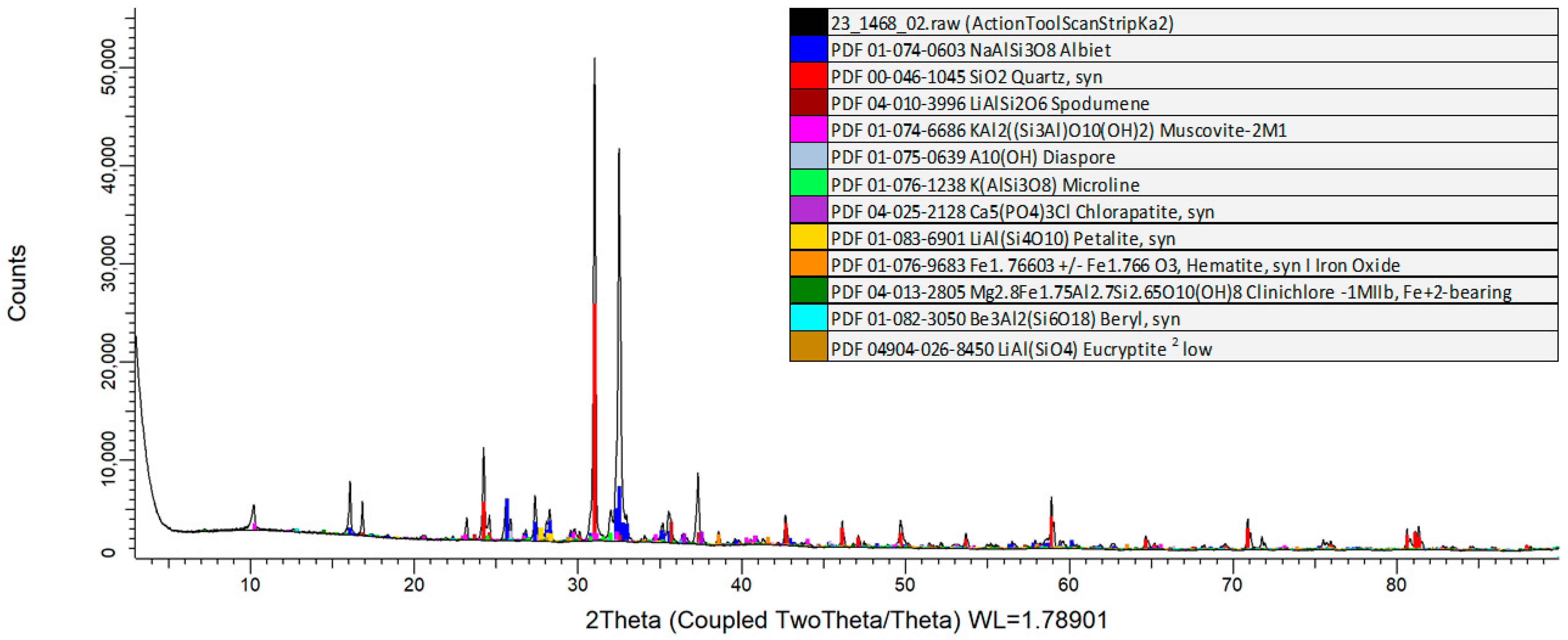
Appendix C. XRD Data for Product and Reject
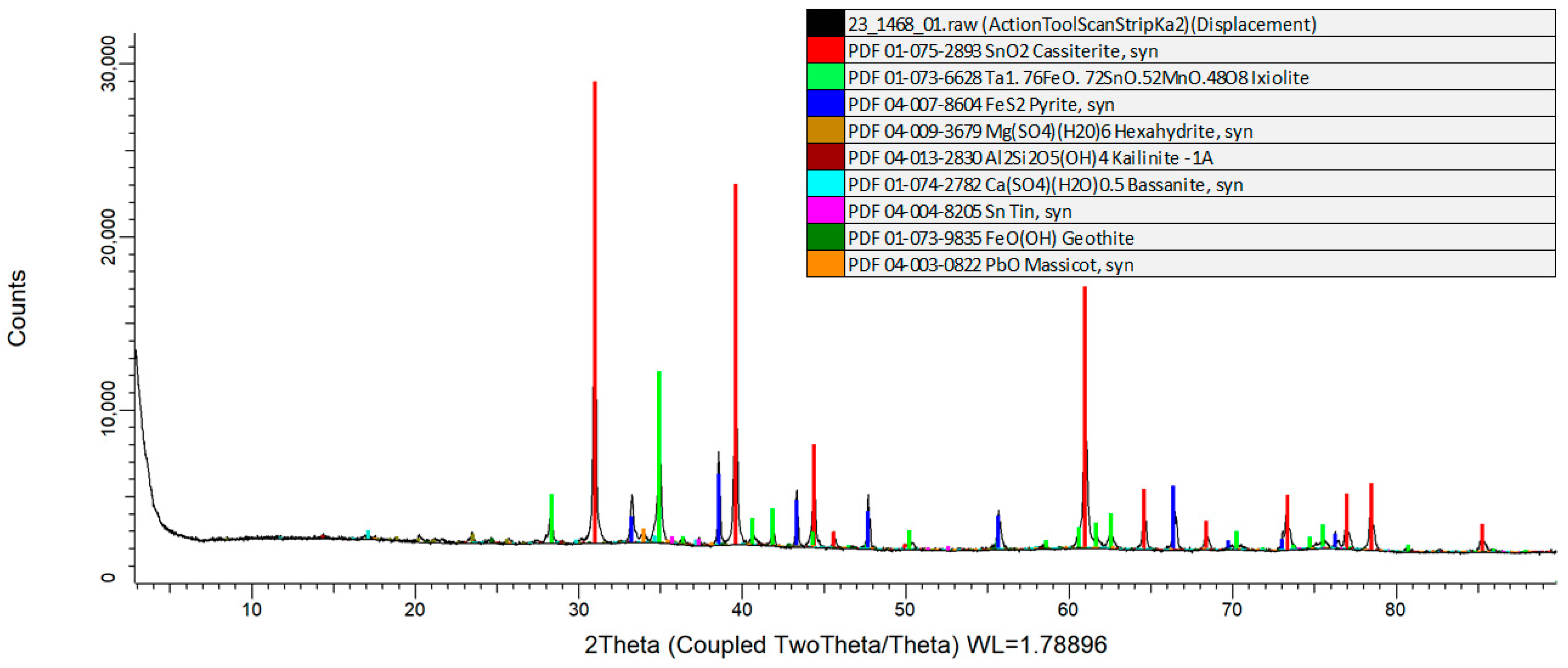
| Crystalline Mineral Phase | Concentration (wt.%) | ICDD Match Probability |
|---|---|---|
| Product Sample: | ||
| Cassiterite, syn (SnO2) | 44 | High |
| Ixiolite (Ta1.76Fe0.72Sn0.52Nb0.52Mn0.48O8) | 22 | High |
| Pyrite, syn (FeS2) | 22 | High |
| Kaolinite-1A (Al2Si2O5(OH)4) | 4 | Low |
| Hexahydrite, syn (Mg(SO4)(H2O)6) | 4 | Low |
| Bassanite, syn (Ca(SO4)(H2O)0.5) | 3 | Low |
| Tin, syn (Sn) | 1 | Low |
| Goethite (FeO(OH)) | 1 | Low |
| Massicot, syn (PbO) | Trace | Low |
| Reject Sample: | ||
| Albite (NaAlSi3O8) | 38 | High |
| Quartz, syn (SiO2) | 29 | High |
| Spodumene (LiAlSi2O6) | 10 | High |
| Muscovite-2M1 (KAl2((Si3Al)O10(OH)2)) | 6 | Medium |
| Microcline (K(AlSi3O8)) | 5 | Medim |
| Chlorapatite, syn (Ca5(PO4)3Cl) | 5 | Low |
| Diaspore (AlO(OH)) | 3 | Low |
| Petalite, syn (LiAl(Si4O10)) | 2 | Low |
| Hematite, syn | Iron Oxide (Fe1.766O3) | 2 | Low |
| Clinochlore-1MIIb, Fe+2-bearing (Mg2.8Fe1.75Al2.7Si2.65O10(OH)8) | 1 | Low |
| Beryl, syn (Be3Al2(Si6O18)) | Trace | Low |
| Eucryptite low (LiAl(SiO4)) | Trace | Low |
References
- Central Coast Consulting. LST Heavy Liquid—Comparison with Other Heavy Liquids. Available online: https://www.chem.com.au/comparison.html (accessed on 15 December 2023).
- Rosenblum, S. A mineral separation procedure using hot Clerici solution. J. Res. U.S. Geol. Survey 1974, 2, 479–481. [Google Scholar]
- Partition Enterprises. Density Tracers. Available online: www.partitionenterprises.com.au/tracers/ (accessed on 15 December 2023).
- Cole, M.J.; Galvin, K.P.; Dickinson, J.E. Maximizing recovery, grade and throughput in a single stage Reflux Flotation Cell. Min. Eng. 2021, 163, 106761. [Google Scholar] [CrossRef]
- Boycott, A.E. Sedimentation of blood corpuscles. Nature 1920, 104, 532. [Google Scholar] [CrossRef]
- Galvin, K.P.; Doroodchi, E.; Callen, A.M.; Lambert, N.; Pratten, S.J. Pilot plant trial of the reflux classifier. Min. Eng. 2002, 15, 19–25. [Google Scholar] [CrossRef]
- Tripathy, S.K.; Bhoja, S.K.; Kumar, C.R.; Suresh, N. A short review on hydraulic classification and its development in mineral industry. Powder Technol. 2015, 270, 205–220. [Google Scholar] [CrossRef]
- Galvin, K.P.; Liu, H. Role of inertial lift in elutriating particles according to their density. Chem. Eng. Sci. 2011, 66, 3687–3691. [Google Scholar] [CrossRef]
- Amariei, D.; Michaud, D.; Paquet, G.; Lindsay, M. The use of the Reflux Classifier for iron ores: Assessment of fine particles recovery at pilot scale. Min. Eng. 2014, 62, 66–73. [Google Scholar] [CrossRef]
- Hunter, D.M.; Zhou, J.; Iveson, S.M.; Galvin, K.P. Gravity separation of ultra-fine iron ore in the REFLUX™ Classifier. Min. Proc. Extr. Metal. C 2016, 125, 126–131. [Google Scholar] [CrossRef]
- Rodrigues, A.F.d.V.; Delboni Junior, H.; Rodrigues, O.M.S.; Zhou, J.; Galvin, K.P. Gravity separation of fine itabirite iron ore using the Reflux Classifier–Part I–Investigation of continuous steady state separations across a wide range of parameters. Min. Eng. 2023, 201, 108187. [Google Scholar] [CrossRef]
- Galvin, K.P.; Zhou, J.; Price, A.J.; Agrwal, P.; Iveson, S.M. Single-stage recovery and concentration of mineral sands using a REFLUX™ Classifier. Min. Eng. 2016, 93, 32–40. [Google Scholar] [CrossRef]
- Galvin, K.P.; Zhou, J.; Sutherland, J.L.; Iveson, S.M. Enhanced recovery of zircon using a REFLUX™ Classifier with an inclined channel spacing of 3 mm. Min. Eng. 2020, 147, 106148. [Google Scholar] [CrossRef]
- Chu, H.; Wang, Y.; Lu, D.; Liu, Z.; Zheng, X. Pre-concentration of fine antimony oxide tailings using an agitated reflux classifier. Powder Technol. 2020, 376, 565–572. [Google Scholar] [CrossRef]
- Galvin, K.P.; Iveson, S.M.; Zhou, J.; Lowes, C.P. Influence of inclined channel spacing on dense mineral partition in a REFLUX™ Classifier. Part 1: Continuous steady state. Min. Eng. 2020, 146, 106112. [Google Scholar] [CrossRef]
- Walton, K.; Zhou, J.; Galvin, K.P. Processing of fine particles using closely spaced inclined channels. Adv. Powder Technol. 2010, 21, 386–391. [Google Scholar] [CrossRef]
- Hunter, D.M.; Iveson, S.M.; Galvin, K.P. The role of viscosity in the density fractionation of particles in a laboratory-scale REFLUX™ Classifier. Fuel 2014, 129, 188–196. [Google Scholar] [CrossRef]
- Galvin, K.P.; Iveson, S.M.; Zhou, J.; Lowes, C.P. Influence of inclined channel spacing on dense mineral partition in a REFLUX™ Classifier. Part 2: Water based fractionation. Min. Eng. 2020, 155, 106442. [Google Scholar] [CrossRef]
- Lowes, C.P.; Zhou, J.; Galvin, K.P. Improved density fractionation of minerals in the REFLUX™ Classifier using LST as a novel fluidising medium. Min. Eng. 2020, 146, 106145. [Google Scholar] [CrossRef]
- Galvin, K.P.; Iveson, S.M.; Hunter, D.M. Deconvolution of fractionation data to deduce consistent washability and partition curves for a mineral separator. Min. Eng. 2018, 125, 94–110. [Google Scholar] [CrossRef]
- Kelly, E.G.; Spottiswood, D.J. Introduction to Mineral Processing; Australian Mineral Foundation: Adelaide, Australia, 1995. [Google Scholar]
- Wills, B.A.; Napier-Munn, T.J. Will’s Mineral Processing Technology, 7th ed.; Butterworth-Heinemann: Oxford, UK, 2006. [Google Scholar]
- Iveson, S.M.; Galvin, K.P. Amplification in the Uncertainty of the Yield and Recovery for a Steady-State Mineral Separator calculated using the Two-Product Formula. ChemRxiv 2023. [CrossRef]
- Available online: www.webmineral.com (accessed on 15 December 2023).


| Sample | Mass Fraction | Balance Yield | Density | Li2O | Fe2O3 | Al2O3 | SiO2 | TiO2 | Mn | S | P | Sn | Ta2O5 | Nb2O5 | Na2O | PbO | CaO | MgO | K2O | Rb | U3O8 | ThO2 | LOI |
|---|---|---|---|---|---|---|---|---|---|---|---|---|---|---|---|---|---|---|---|---|---|---|---|
| (wt.%) | (wt.%) | (RD) | (wt.%) | (wt.%) | (wt.%) | (wt.%) | (wt.%) | (wt.%) | (wt.%) | (wt.%) | (wt.%) | (wt.%) | (wt.%) | (wt.%) | (wt.%) | (wt.%) | (wt.%) | (wt.%) | (wt.%) | (wt.%) | (wt.%) | (wt.%) | |
| Head samples: | |||||||||||||||||||||||
| Feed | 2.8102 | 0.828 | 1.880 | 15.130 | 66.240 | 0.105 | 0.118 | 0.808 | 0.801 | 1.296 | 0.561 | 0.199 | 4.040 | 0.015 | 3.320 | 0.500 | 1.436 | 0.094 | 0.007 | 0.002 | 1.29 | ||
| Product | 0.255 | 16.400 | 1.750 | 4.280 | 0.324 | 1.326 | 12.258 | 0.222 | 34.553 | 13.305 | 4.359 | 0.160 | 0.214 | 1.200 | 0.140 | 0.141 | 0.006 | 0.163 | 0.014 | 7.78 | |||
| Reject | 0.858 | 1.260 | 15.780 | 68.550 | 0.098 | 0.062 | 0.283 | 0.827 | 0.065 | 0.068 | 0.027 | 4.250 | 0.004 | 3.320 | 0.530 | 1.467 | 0.094 | 0.002 | 0.001 | 0.98 | |||
| Yield (wt.%) | 4.0 | 5.0 | 4.1 | 4.6 | 3.6 | 3.1 | 4.4 | 4.4 | 4.3 | 3.6 | 3.7 | 4.0 | 5.1 | 5.2 | 0.00 | 7.7 | 2.3 | −0.8 | 3.1 | 4.5 | 4.6 | ||
| Recovery (%) | 1.5 | 35.7 | 0.5 | 0.2 | 9.6 | 49.8 | 66.5 | 1.2 | 95.2 | 88.3 | 87.0 | 0.2 | 74.7 | 0.00 | 2.2 | 0.2 | −0.1 | 69.5 | 31.5 | 27.5 | |||
| Upgrade (-) | 0.3 | 8.7 | 0.1 | 0.1 | 3.1 | 11.2 | 15.2 | 0.3 | 26.7 | 23.7 | 21.9 | 0.0 | 14.3 | 0.4 | 0.3 | 0.1 | 0.1 | 22.3 | 6.9 | 6.03 | |||
| Yield Error Amplification, AY (-) | 39.0 | 4.3 | 32.9 | 40.6 | 21.2 | 3.0 | 2.2 | 43.6 | 1.5 | 1.6 | 1.6 | 27.2 | 1.9 | Error | 23.6 | 65.5 | 190.7 | 2.1 | 5.0 | 5.9 | |||
| Recovery Error Amplification, AR (-) | 40.4 | 2.9 | 34.3 | 42.0 | 19.8 | 1.6 | 0.8 | 45.0 | 0.1 | 0.2 | 0.2 | 28.6 | 0.5 | Error | 25.0 | 66.9 | 189.3 | 0.7 | 3.6 | 4.5 | |||
| +0.045 mm wet-screened samples: | |||||||||||||||||||||||
| Feed | 93.1 | 2.8102 | 0.777 | 1.81 | 15.11 | 66.62 | 0.104 | 0.103 | 0.761 | 0.792 | 1.257 | 0.527 | 0.176 | 4.11 | 0.011 | 3.27 | 0.50 | 1.416 | 0.091 | 0.008 | 0.003 | 1.22 | |
| Product | 93.8 | 5.4846 | 0.327 | 18.16 | 2.11 | 5.28 | 0.338 | 1.205 | 11.534 | 0.266 | 32.182 | 12.486 | 4.017 | 0.19 | 0.200 | 1.35 | 0.17 | 0.153 | 0.006 | 0.132 | 0.012 | 8.65 | |
| Reject | 86.1 | 2.7609 | 0.829 | 1.08 | 15.64 | 69.56 | 0.096 | 0.054 | 0.236 | 0.801 | 0.048 | 0.045 | 0.019 | 4.33 | 0.004 | 3.29 | 0.49 | 1.430 | 0.096 | 0.002 | 0.001 | 0.86 | |
| Yield (wt.%) | 4.1 | 10.4 | 4.3 | 3.9 | 4.6 | 3.3 | 4.3 | 4.6 | 1.7 | 3.8 | 3.9 | 3.9 | 5.3 | 3.6 | 1.0 | −3.1 | 1.1 | 4.9 | 4.8 | 10.5 | 4.6 | ||
| Recovery (%) | 4.4 | 42.9 | 0.5 | 0.4 | 10.7 | 49.8 | 70.4 | 0.6 | 96.3 | 91.8 | 89.6 | 0.2 | 64.9 | 0.4 | −1.1 | 0.1 | 0.3 | 80.6 | 49.1 | 32.8 | |||
| Upgrade (-) | 0.4 | 10.0 | 0.1 | 0.1 | 3.3 | 11.7 | 15.2 | 0.3 | 25.6 | 23.7 | 22.8 | 0.0 | 18.2 | 0.4 | 0.3 | 0.1 | 0.1 | 16.8 | 4.7 | 7.1 | |||
| Yield Error Amplification, AY (-) | 21.1 | 3.5 | 40.3 | 32.0 | 18.4 | 3.0 | 2.0 | 124.5 | 1.5 | 1.5 | 1.6 | 26.4 | 2.2 | 231.2 | 70.7 | 143.0 | 29.3 | 1.8 | 3.3 | 4.8 | |||
| Recovery Error Amplification, AR (-) | 22.5 | 2.1 | 41.7 | 33.5 | 17.0 | 1.6 | 0.6 | 125.9 | 0.1 | 0.1 | 0.2 | 27.8 | 0.8 | 232.6 | 69.3 | 144.5 | 30.7 | 0.4 | 1.9 | 3.4 | |||
| −0.045 mm wet-screened samples: | |||||||||||||||||||||||
| Feed | 6.9 | 0.776 | 3.78 | 15.12 | 57.66 | 0.189 | 0.311 | 0.911 | 0.988 | 3.658 | 1.793 | 0.584 | 3.74 | 0.049 | 4.10 | 0.73 | 1.399 | 0.082 | 0.031 | 0.005 | 1.71 | ||
| Product | 6.2 | 0.014 | 4.63 | 0.31 | 1.21 | 0.260 | 1.944 | 1.810 | 0.023 | 50.691 | 18.271 | 5.339 | 0.05 | 0.385 | 0.47 | 0.03 | 0.080 | 0.003 | 0.341 | 0.025 | 1.36 | ||
| Reject | 13.9 | 0.880 | 3.71 | 17.06 | 59.63 | 0.192 | 0.193 | 0.632 | 1.112 | 0.812 | 0.607 | 0.216 | 3.79 | 0.033 | 4.46 | 0.91 | 1.752 | 0.096 | 0.016 | 0.004 | 1.84 | ||
| Yield (wt.%) | 6.0 | 12.0 | 7.6 | 11.6 | 3.4 | −4.4 | 6.7 | 23.7 | 11.4 | 5.7 | 6.7 | 7.2 | 1.3 | 4.5 | 9.0 | 20.5 | 21.1 | 15.5 | 4.4 | 2.0 | 27.1 | ||
| Recovery (%) | 0.2 | 9.3 | 0.2 | 0.1 | −6.1 | 42.1 | 47.1 | 0.3 | 79.1 | 68.4 | 65.7 | 0.02 | 35.7 | 1.0 | 0.8 | 1.2 | 0.6 | 49.2 | 10.7 | 21.5 | |||
| Upgrade (-) | 0.0 | 1.2 | 0.0 | 0.0 | 1.4 | 6.3 | 2.0 | 0.0 | 13.9 | 10.2 | 9.1 | 0.01 | 7.9 | 0.1 | 0.0 | 0.1 | 0.0 | 11.1 | 5.5 | 0.8 | |||
| Yield Error Amplification, AY (-) | 10.6 | 76.4 | 11.0 | 41.4 | 89.1 | 3.7 | 4.6 | 11.3 | 1.8 | 2.1 | 2.2 | 105.8 | 4.3 | 16.1 | 5.7 | 5.6 | 8.0 | 3.0 | 15.9 | 18.6 | |||
| Recovery Error Amplification, AR (-) | 12.0 | 75.0 | 12.4 | 42.8 | 90.5 | 2.3 | 3.2 | 12.7 | 0.4 | 0.7 | 0.8 | 107.2 | 2.9 | 17.5 | 7.1 | 7.0 | 9.5 | 1.6 | 14.5 | 20.0 | |||
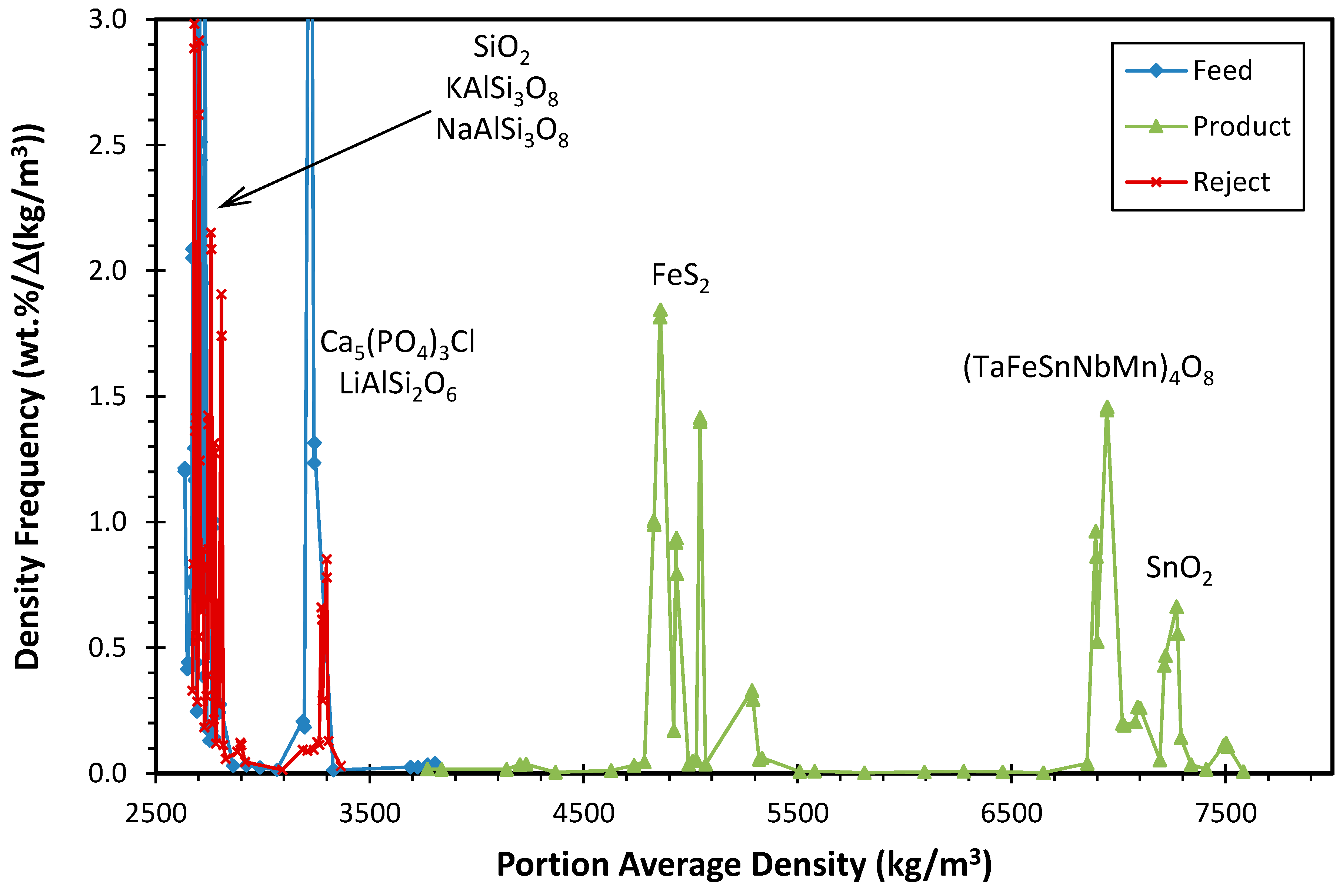
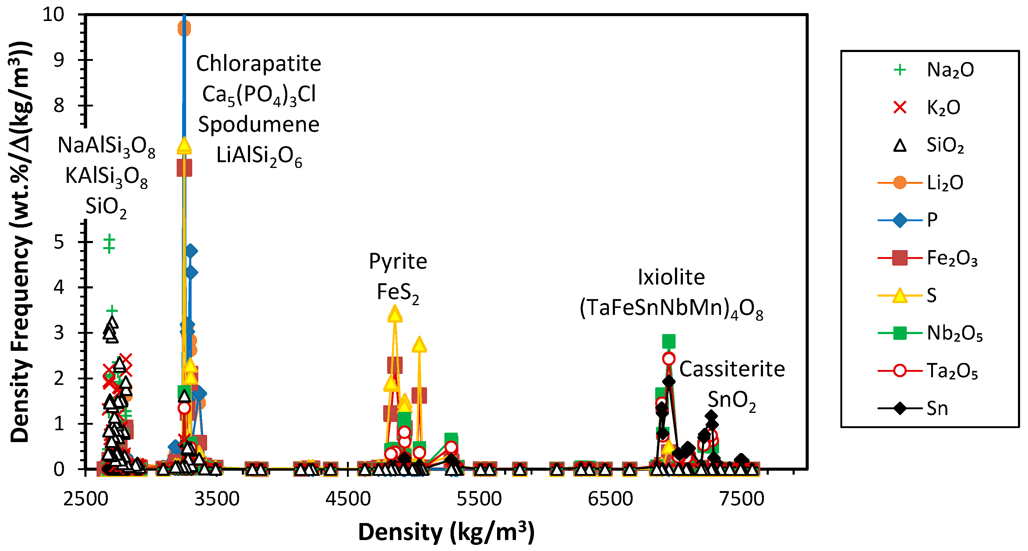
| XRF Label | Likely Actual Mineral (Based on XRD) | Peak Densities in Figure 11 (kg/m3) | Average Density, rav,i (kg/m3) | Literature Density (kg/m3) | Literature Density Source |
|---|---|---|---|---|---|
| Sn | Cassiterite SnO2 | 7270, 6947, 6893 | 6936 UF Product | 6800–7100 | [21] |
| Ta2O5 Nb2O5 | Ixiolite (TaFeSnNbMn)4O8 | Ta 6947, 3253 Nb 6947, 6893, 4931, 3253 | Ta 6559 Nb 6387 UF Product | 6940–7230 | [23] |
| Fe2O3 S | Pyrite FeS2 | 5044, 4859, 3298, 3253 | Fe 3783 S 4272 | 5000 | [21] |
| P | Chlorapatite Ca5(PO4)3Cl | 3253 | OF Reject 3239 | 3100–3200 | [23] |
| Li2O | Spodumene LiAlSi2O6 | 3253, 2807 | OF Reject 3191 | 3100–3200 | [21] |
| SiO2 | Quartz SiO2 | 2759, 2703 | OF Reject 2794 | 2650–2660 | [21] |
| K2O | Microcline KAlSi3O8 | 2807, 2749, 2680 | OF Reject 2770 | 2560 | [23] |
| Na2O | Albite NaAlSi3O8 | 2745, 2681 | OF Reject 2743 | 2600–2700 | [21] |
Disclaimer/Publisher’s Note: The statements, opinions and data contained in all publications are solely those of the individual author(s) and contributor(s) and not of MDPI and/or the editor(s). MDPI and/or the editor(s) disclaim responsibility for any injury to people or property resulting from any ideas, methods, instructions or products referred to in the content. |
© 2024 by the authors. Licensee MDPI, Basel, Switzerland. This article is an open access article distributed under the terms and conditions of the Creative Commons Attribution (CC BY) license (https://creativecommons.org/licenses/by/4.0/).
Share and Cite
Iveson, S.M.; Boonzaier, N.; Galvin, K.P. Beneficiation of High-Density Tantalum Ore in the REFLUX™ Concentrating Classifier Analysed Using Batch Fractionation Assay and Density Data. Minerals 2024, 14, 197. https://doi.org/10.3390/min14020197
Iveson SM, Boonzaier N, Galvin KP. Beneficiation of High-Density Tantalum Ore in the REFLUX™ Concentrating Classifier Analysed Using Batch Fractionation Assay and Density Data. Minerals. 2024; 14(2):197. https://doi.org/10.3390/min14020197
Chicago/Turabian StyleIveson, Simon M., Nicolas Boonzaier, and Kevin P. Galvin. 2024. "Beneficiation of High-Density Tantalum Ore in the REFLUX™ Concentrating Classifier Analysed Using Batch Fractionation Assay and Density Data" Minerals 14, no. 2: 197. https://doi.org/10.3390/min14020197
APA StyleIveson, S. M., Boonzaier, N., & Galvin, K. P. (2024). Beneficiation of High-Density Tantalum Ore in the REFLUX™ Concentrating Classifier Analysed Using Batch Fractionation Assay and Density Data. Minerals, 14(2), 197. https://doi.org/10.3390/min14020197