Abstract
Quartz is an important mineral in many metal deposits and can provide important indications about the deposit's origin through its chemical composition. However, traditional low-dimensional analysis methods are ineffective in utilizing quartz's chemical composition to reveal the deposit's origin type. In this study, 1140 quartz samples from eight geological environments were collected, and three machine learning (ML) models—random forest, eXtremely Greedy tree Boosting (XGBoost), and light gradient boosting machine (LightGBM) were used to classify quartz deposits. The application of the Shapley Additive Explanation (SHAP) algorithm and Spearman correlation analysis is utilized to interpret the predictive results of the model and analyze feature correlations, aiming to enhance the credibility of the classification results and discover underlying patterns. Finally, a visualization method based on XGBoost and t-SNE was proposed. By calculating SHAP values, the key geochemical indicators that differentiate each type of quartz deposit were determined. Furthermore, the impact of varying concentrations of different trace elements on the identification of quartz deposits was analyzed. This study demonstrated the effectiveness of using machine-learning algorithms based on trace elements to classify quartz and provided new insights into the relationships between trace elements and quartz genesis, as well as the effects of different trace element combinations and concentrations on quartz identification.
1. Introduction
Quartz is an extremely important mineral resource that is widely distributed in volcanic, plutonic, metamorphic, diagenetic, and metallogenic environments [1,2]. Quartz is an important mineral in many metal deposits, and its chemical composition can provide important indications about the source of the deposit. The trace element concentrations of quartz can reflect the physicochemical conditions during quartz growth and the regional geological evolution process [3,4,5]. Analyzing the trace elements of quartz can help identify the genetic environment of quartz and further explore the exploration potential of the region [6,7,8,9]. The Ti-Al/50-10Ge ternary diagram can be used to classify quartz from granites, pegmatites, and rhyolites [10]. Quartz from epithermal, orogenic, and porphyry (Cu-Mo-Au) deposits can be discriminated against using the Ti-Al binary diagram [11]. Two-dimensional identification diagrams are a mature technique in the field of mineralogy for describing the physical and chemical properties of ores. This method can visualize the trend and pattern of mineral deposits, identify key mineralogical and geochemical features, and help understand their deposits and exploitation potential. Subsequent studies have shown that this method has significant limitations, making it difficult to consider the role of various trace elements in the study [12,13,14,15]. As a result, the results may be inaccurate. In terms of quartz genesis discrimination, the limitations of binary and ternary diagrams in representing high-dimensional information also restrict their application in many scenarios [16]. For example, in the quartz data studied by [17], most of the C-type, D-type, and E-type quartz from porphyry deposits fall outside the area of porphyry deposits defined by the Ti-Al diagram of [11]. Trace element data for granitic quartz studied by [18] were determined to fall outside the granite range of the Ti-Al-Ge ternary diagram of [10].
In recent times, the progress in artificial intelligence has resulted in an increasing prevalence of machine learning techniques in geological research, particularly in the field of tectonic environment identification [19,20,21,22]. Research indicates that machine-learning algorithms exhibit good performance in feature analysis of rock samples from various tectonic environments [23,24]. However, these algorithms have limitations in recognizing ore deposits, including challenges in visualizing classification results and interpreting the models [25]. Typically, the classification results are usually in the form of numbers or labels, which do not intuitively reflect the origin of the deposit [16]. Consequently, there is a need to develop visualization methods to overcome this challenge. In addition, the lack of interpretability in machine learning restricts the usability of ML models in general scientific tasks, such as understanding hidden causal relationships, obtaining actionable insights, and generating new scientific hypotheses [26]. The remedy for this issue lies in interpretable machine learning. Interpretable machine learning refers to the ability of machine-learning models to explain their predictions or decisions in an understandable and transparent manner [27]. In recent years, interpretable machine learning has gained popularity in research fields such as healthcare, materials science, economics, and chemistry [26,28,29,30]. In the field of ore deposit discrimination, the lack of emphasis on model interpretability in previous methods has turned the models into black boxes, posing challenges for researchers. Providing explanations for models can help geologists understand the decision-making process and important features and discover new geological knowledge. This aids in enhancing the credibility and accuracy of the models, allowing for better application in geological research and mineral exploration.
In this study, machine learning and quartz geochemical data were utilized to distinguish quartz samples from different deposits. Random forest [31], XGBoost, and LightGBM-based quartz classifiers were designed to distinguish quartz samples from eight types of ore deposits, including epithermal, greisen, Carlin, porphyry, pegmatite, skarn, orogenic, and granite. All three methods were successfully applied to classify tectonic environments of rock samples [20,22,23,24,32,33]. We employ the Shapley Additive Explanations (SHAP) [34] technique to interpret the quartz classification model. This technique utilizes game theory to provide explanations for machine-learning predictions [35]. This method has been widely applied for interpreting machine-learning models in various domains, such as accident detection [36], prediction of medical compound activity [37,38], and structural fault prediction [38]. Regarding the issue of data imbalance in the compiled quartz geochemical data, the Synthetic Minority Over-sampling Technique (SMOTE) [39] was introduced to perform data augmentation on the dataset. This technique was used to address the problem of insufficient samples in the minority class by creating synthetic samples that are similar to the original ones. In addition, Spearman's correlation was calculated to analyze the correlation between trace elements in quartz samples from different origins. Finally, a binary visualization scheme based on XGBoost and t-Distributed Stochastic Neighbor Embedding (t-SNE) [40,41,42] was presented, which allowed for the two-dimensional visualization of the quartz samples from different deposits to facilitate the intuitive presentation of the classification results. We use accuracy, recall, confusion matrix, and learning curves as evaluation metrics for the quartz classifiers.
Our study demonstrates that the quartz classifiers perform well in multiple evaluation metrics, with the XGBoost-based classifier being the most effective. This confirms that machine-learning models can accurately classify quartz samples from different deposits, providing a reliable method for provenance identification. The binary visualization scheme based on XGBoost and t-SNE facilitates the intuitive and accurate identification of the origin of quartz samples. Additionally, by applying SHAP to interpret the quartz classification models, we enhance the acceptability and trustworthiness of the prediction results and facilitate the discovery of underlying patterns. The analysis of feature correlations reveals significant associations among certain trace elements in quartz samples from different tectonic backgrounds. For instance, there is a positive correlation between Al and Li, Al, and Na, as well as Al and K. In epithermal quartz samples, there is a negative correlation between Ge and P.
2. Compiled Data
The current study employs a dataset consisting of quartz trace element information obtained from eight different deposits sourced from thirty-one regions worldwide. The use of quartz geochemical data from a diverse range of global deposits increases the generalizability of the model being proposed. Detailed data sources can be found in the references listed in Table 1.

Table 1.
Composition and source of the collected dataset.
The trace element analysis of the quartz samples was performed using ambient laser ablation inductively coupled plasma mass spectrometry (LA-ICP-MS). The geographic locations of quartz samples from eight different deposits are shown in Figure 1. The trace element data were gathered from various deposits, including porphyry, pegmatite, granite, skarn, epithermal, carlin, greisen, and orogenic deposits. The study focuses on eight selected trace elements—Al, Ti, Li, Ge, Fe, Na, K, and P, to characterize the training samples. The eight selected trace elements are crucial microelements in quartz, commonly found in quartz samples, and have been previously identified as significant indicators of different deposit types [10,11,41,42]. The dataset was filtered to exclude samples that did not contain all eight elements, resulting in 1140 remaining quartz samples, comprising porphyry (n = 193), epithermal (n = 167), greisen (n = 84), carlin (n = 121), pegmatite (n = 34), skarn (n = 433), granite (n = 43), and orogenic (n = 64) deposits. Figure 2 illustrates the compilation of trace element information for quartz from various deposits. Quartz encompasses a range of trace element distributions, and its constructional environment can be differentiated through the analysis of its trace element composition (Figure 2). The trace element Al demonstrates a higher degree of abundance in quartz sourced from various deposits, while the distribution range of P is comparatively limited within quartz samples (Figure 2).
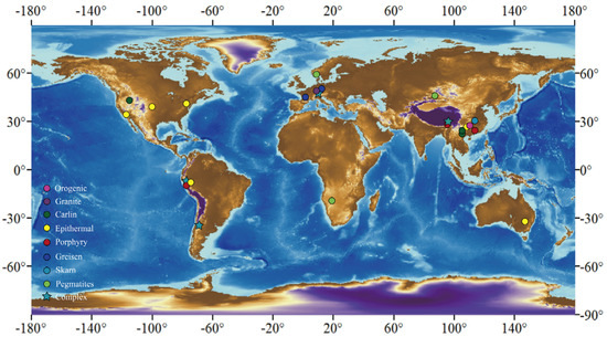
Figure 1.
Map of the global distribution of quartz samples. 'Complex' indicates the inclusion of multiple types of quartz.
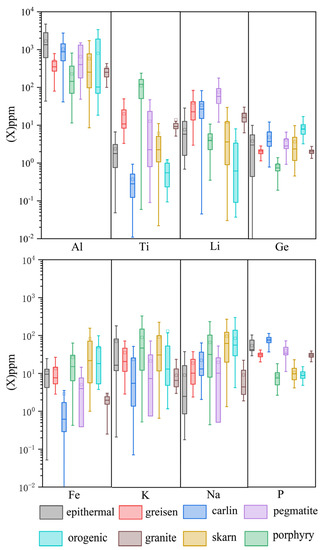
Figure 2.
Map of the trace element content of different types of quartz. The height of the colored bars represents the range of quartiles. The black borders and white dots represent the mean value, while the horizontal black line within each colored bar represents the median. The “whiskers” of each box indicate the extreme values that fall within 1.5 times the interquartile range outside the edges of the bars.
3. Methods
The workflow consists of three steps (Figure 3). Firstly, a preprocessing was executed, which comprised normalizing and transforming the selected dataset using Gaussian distribution. The data were partitioned into training and testing subsets in 8:2 proportion. In order to address the issue of data imbalance, data augmentation is performed to expand the dataset. Data augmentation allows for more widespread distribution of minority class samples in the feature space, thereby enhancing the model’s learning capability towards the minority class. In this study, the SMOTE algorithm is chosen as the method to implement data augmentation. In the second step, three classifiers were developed using three machine-learning algorithms, and the model parameters were optimized through grid search methodology, resulting in the development of a high-quality quartz classifier. The performance of the three quartz classifiers was compared based on evaluation metrics. A feature importance analysis of the trace elements present in the quartz samples was conducted using SHAP values. Finally, a two-dimensional discriminant map was generated to visually differentiate quartz originating from varying deposits through the construction of decision boundaries based on machine-learning algorithms.
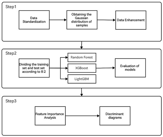
Figure 3.
Operational flow chart of the operation of the research method. Step 1: Data preprocessing and data augmentation. Step 2: Dataset partitioning and training of three classifiers. Step 3: Feature importance analysis and visualization.
3.1. Data Preprocessing
The process of data preprocessing is a critical step in improving the quality of the data. By normalizing, transforming, and augmenting the dataset, the accuracy and efficiency of subsequent classification are enhanced. This is particularly important in the context of machine learning, as the quality of the input data has a direct impact on the performance of the model. In supervised multi-label classification, the training set is used for training the classification model, and the test set is used to evaluate the trained classification model. The quartz dataset was divided into a training set and a test set in the ratio of 8:2. The function of the training set is to train the classifier, and the function of the test set is to verify the classification effect of the classifier on the new data. In order to better solve the problem of quartz classification, we standardize the data. Through standardization, different characteristic variables can have the same scale, in order to eliminate the difference between features, accelerate the convergence speed, and improve the accuracy of classification [60]. In addition, the Gaussian transformation is carried out on the quartz dataset to alleviate the influence of data distribution tilt and make the original dense interval as scattered as possible. According to the data sample distribution described in Figure 4. It can be seen that there must be data imbalance in quartz datasets, which may affect the final quartz classification results [61,62]. Therefore, we use SMOTE algorithm to alleviate the imbalance of datasets. Figure 5 illustrates the ten-fold cross-validation curves for the three methods before and after the dataset undergoes SMOTE processing. Ten-fold cross-validation is widely used as it helps to reduce the uncertainty in the selection of the validation set [63,64]. It can be observed that, through the application of SMOTE, there is a significant improvement in the model performance, indicating that SMOTE effectively mitigates the issue of data imbalance.
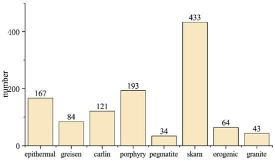
Figure 4.
Distribution of different quartz species in datasets.
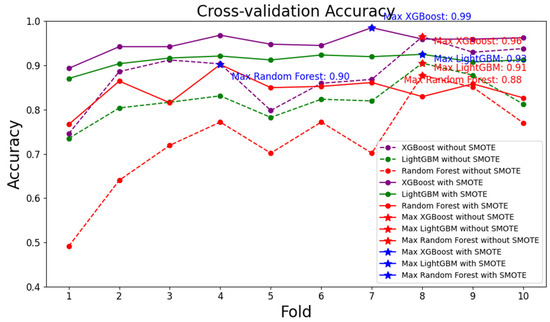
Figure 5.
Ten-fold cross-validation curves for the three methods before and after SMOTE Processing of the dataset.
3.2. Building Classifiers
Random Forest [31] is a type of supervised machine-learning algorithm that consists of an ensemble of multiple decision trees. The method utilizes bootstrapping techniques to randomly select training samples from the dataset, leading to the creation of diverse decision trees and training subsets. Due to its accuracy, versatility, and simplicity, Random Forest has gained widespread utilization across various fields. Additionally, its capability to handle nonlinear relationships between variables and its efficiency in the analysis of diverse datasets further add to its appeal.
XGBoost [65] is an optimized and distributed gradient-boosting library that allows for the scalable and efficient training of machine-learning models. As an integrated learning method, XGBoost combines the predictions of multiple weak models to improve overall prediction results. It has demonstrated exceptional performance in handling large datasets. XGBoost has gained widespread popularity in various data analysis tasks, in part due to its ability to handle missing values in real data, obviating the need for elaborate preprocessing steps. The algorithm is based on gradient-boosting decision trees, where decision trees are constructed sequentially and assigned weights, which play a crucial role in XGBoost. These weights are assigned to all independent variables and fed into the decision tree, with the weights of the variables that are incorrectly predicted by the tree being increased and fed into subsequent decision trees. The final prediction is the result of the integration of these individual predictions, resulting in robust and accurate outcomes.
LightGBM [66] is a gradient-boosting framework that is based on the widely used decision tree algorithm. This framework is characterized by its fast speed, distributed nature, and high performance. It uses a unique approach to growing decision trees, where it grows by leaves and selects the leaf with the maximum incremental value. This approach leads to several advantages, including reduced memory usage, decreased cost of parallel learning, and a lower computational cost associated with calculating the gain per split in the decision tree. These features make LightGBM a highly efficient and appealing choice for various data analysis tasks.
The optimization of parameters is a crucial step in improving the performance of a classification model. It entails determining the optimal settings for the input variables by exploring a range of possible values. This process is typically accomplished through the use of grid search and K-fold cross-validation. In grid search, various combinations of parameter values are evaluated, and the best combination is selected based on the minimizing of the loss function on the training set. The "early stop" method, as proposed by [67], can be employed to expedite the tuning process and identify the optimal combination of parameters efficiently.
Recall, F1-score, and accuracy were chosen as evaluation metrics for multiple quartz classifiers. Recall denotes how many of the samples predicted to be positive are true positive samples. Precision denotes how many of the positive samples in the sample are predicted to be correct. F1-score can be interpreted as a weighted average of recall and accuracy. Furthermore, two evaluation metrics, namely confusion matrices and learning rate curves, are introduced for evaluating classifiers. A confusion matrix provides a comprehensive representation of the prediction results, where it categorizes the number of correct and incorrect predictions and summarizes them [68]. The learning curve, on the other hand, depicts the alteration of the model's performance scores on the training and validation datasets as the size of the training set increases [69]. The learning curve can serve as a diagnostic tool to detect overfitting or underfitting issues in the model.
3.3. Feature Importance Analysis
Feature importance analysis aims to quantify the relative importance of each feature in making predictions by a model [70]. By conducting feature importance analysis, one can gain a deeper understanding of the data distribution and enhance the interpretability of the classification model. The results of the analysis can be used to improve the prediction model. In this study, the SHAP method, which is a game-theoretic-based approach for explaining the output of machine-learning models and enhancing their interpretability, was utilized for the feature importance analysis. The fundamental principle of the SHAP method is that the effect of individual features on the target variable is influenced by both the features themselves and the complete set of features. To calculate the impact of each feature, the SHAP method leverages combinations of various features. The average absolute value of the impact of a set of features on the target variable can be used as an indicator of their relative significance. It is worth noting that the results produced by the SHAP method are model agnostic and do not depend on the particular model utilized.
4. Results
4.1. Tuning Parameters
Parameter selection represents a critical step in the development of machine-learning models, as it significantly impacts model performance, generalization capabilities, and computational efficiency, thus ensuring better alignment with specific datasets and problem domains. Grid search, through a systematic exploration of the defined parameter combinations, enables the evaluation of all feasible parameter values, ultimately leading to the identification of the optimal parameter configuration. Furthermore, cross-validation provides an effective means to evaluate model performance and mitigate the risks associated with overfitting. In this study, grid search and cross-validation techniques were chosen to optimize the parameters. Detailed information regarding the parameters, their respective ranges, and the optimal values for XGBoost, LightGBM, and Random Forest can be found in Table 2.
Table 2.
Parameter ranges and selected parameter values for the three models.
4.2. Output of Classifier Models
The three classifiers were trained on the pre-processed and data-enhanced dataset, and the model parameters were optimized through a combination of grid search and cross-validation, aimed at achieving optimal results. To visually assess the prediction performance of the models, they were evaluated on the test set using metrics such as precision, recall, F1-score, confusion matrix, and learning curve, respectively.
Learning curves are an important tool for evaluating models. The x-axis of learning curves represents the size of the training set. The y-axis represents the model score, which is generally defined as accuracy, and a higher score indicates better performance. Learning curves are composed of two curves, the training score curve and the cross-validation score curve on the validation set. Figure 6 shows the learning curves of three classifiers. The difference between the training score curve and the cross-validation score curve is relatively small in the three learning curves, indicating that there is no overfitting or underfitting in the three classifiers (Figure 6). The score of the learning curve for the quartz classifier based on the random forest is relatively low, indicating a relatively poor classification performance (Figure 6a).
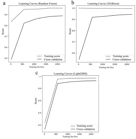
Figure 6.
Learning curves of the three classifiers. (a) Random Forest. (b) XGBoost. (c) LightGBM.
The three classifiers use the same test set. The average prediction accuracy of Random Forest on the test set for eight deposits of quartz was 0.89. XGBoost had a relatively high average prediction accuracy, which can reach 0.95. The prediction accuracy of LightGBM was 0.93. In order to better understand the recognition effect of each classifier on different types of samples, the accuracy, recall, and F1-score of the classifier for the eight deposits were calculated. Figure 7 depicts the prediction accuracy, recall, and F1-score of the three classifiers for eight deposits of quartz. As shown in Figure 7, the overall performance of the random forest classifier is inferior compared to the other two classifiers. The recall and prediction accuracy of the quartz classifier based on the random forest for the different classes in the test set vary greatly, which further highlights the inefficiency of the random forest in terms of prediction accuracy (Figure 7c). The classifier’s recognition of quartz samples from the greisen deposit is poor, with the prediction accuracy of the random forest being only 0.63 (Figure 7c). In contrast, the recognition of quartz samples from the epithermal and carlin deposits is more favorable, with XGBoost having the best performance and achieving 100% recognition (Figure 7b).
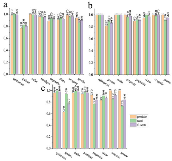
Figure 7.
Precision, recall, and F-score of different classifiers on the test set. (a) LightGBM. (b) XGBoost. (c) Random Forest.
To further analyze the performance of the three classifiers, we utilized confusion matrices. By considering the confusion matrices from the training set, test set, and ten-fold cross-validation, a more comprehensive evaluation of model performance was provided. Combining the results from the three confusion matrices, it can be observed that the random forest classifier performs worse than the other two classifiers, while XGBoost exhibits the best performance (Figure 8). As shown in Figure 8, quartz samples from epithermal, carlin, orogenic, and granite deposits demonstrate good identification performance, indicating that quartz from these types of deposits possesses distinctive trace element distributions. However, these three classifiers struggle to effectively differentiate quartz from greisen deposits and tend to misclassify it as quartz from pegmatite deposits. Similarly, there is a certain probability that quartz from pegmatite deposits is incorrectly classified as quartz from greisen deposits. The overlapping distributions of Al, Ti, Li, Fe, K, Na, and P trace elements in quartz from greisen and pegmatite deposits, as illustrated in Figure 2, further indicate the presence of similarities in their trace element distributions. This suggests that quartz from greisen and pegmatite deposits may exhibit similar trace element distributions.
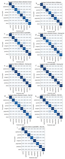
Figure 8.
Average Confusion Matrices Obtained by Three Models through 10-Fold Cross-Validation and Confusion Matrices Obtained on the Training Set and Test Set. (a) Random Forest (10-Fold CV), (b) XGBoost (10-Fold CV), (c) LightGBM (10-Fold CV), (d) Random Forest (Training Set), (e) XGBoost (Training Set), (f) LightGBM (Training Set), (g) Random Forest (Test Set), (h) XGBoost (Test Set), (i) LightGBM (Test Set).
5. Discussion
5.1. Feature Importance Analysis
This study presents an investigation of feature importance overlay bar charts for the Quartz multiclass problem, utilizing three different classifiers: Random Forest, XGBoost, and LightGBM. The feature importance overlay bar chart visually displays the relative importance of each input variable in the classification model (Figure 9). The aim of this analysis is to provide insights into the performance of each classifier in identifying significant input variables and their respective contributions to the classification task. In Figure 9, the features are arranged in descending order of importance based on their mean SHAP values. A higher mean SHAP value indicates greater feature importance. In order to enhance the reliability of the feature analysis conclusions, mean SHAP values of the features were calculated using three machine-learning algorithms. Through three feature importance analyses, it was found that among the eight features, P, Ti, Li, Ge, and Al have a high contribution to the identification of quartz in eight tectonic settings. This finding is consistent with previous related studies [10,11,41]. P and Ti are more important than other trace elements, indicating a significant difference in the distribution of P and Ti in quartz among the eight tectonic settings. P and Ti make a significant contribution to distinguishing quartz from skarn, carlin, and greisen deposits, while they have a smaller contribution to identifying quartz from pegmatite deposits. The mean SHAP value of Li in quartz from pegmatite deposits is relatively high, indicating a unique Li element distribution in quartz from pegmatite deposits. The mean SHAP value of Ge in quartz from orogenic deposits is also relatively high, indicating a distinct Ge element distribution in quartz from orogenic deposits. Fe and Ti have a higher contribution to distinguishing quartz from granite deposits. P has a higher contribution to identifying quartz from epithermal and Carlin deposits compared to other elements. The results suggest that the distribution of certain trace elements, such as P, Ti, Li, Ge, and Al, in quartz varies significantly among different tectonic settings. This information can provide important insights into the geological processes that led to the formation of these deposits.
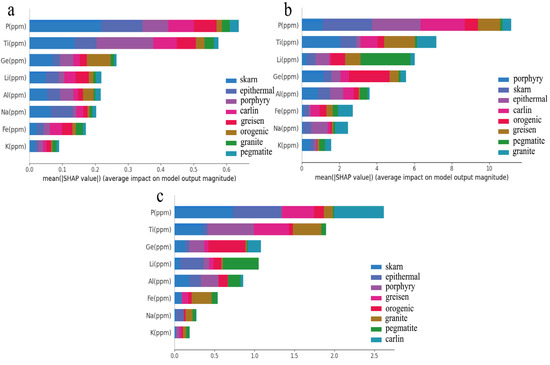
Figure 9.
Stacked bar plot of feature importance for the quartz multi-class problem, comparing (a) random forest classifier, (b) XGBoost classifier, and (c) LightGBM classifier. The bars of different colors in the plot represent different categories of quartz.
When using machine-learning models, features have a significant impact on the prediction results. Not all features are necessary for prediction, and removing redundant features can improve model performance and reduce complexity. Based on the results shown in Figure 9, it is evident that the feature importance of K and Na is significantly lower than that of other features. Therefore, we chose K and Na as variables to investigate the impact of feature selection on the quartz classification model. The results are depicted in Figure 10. Based on Figure 10, we can conclude that the selection of K and Na as features has a minimal influence on the final results of XGBoost. This demonstrates the robustness of the quartz classification model based on XGBoost. As shown in Figure 10, retaining Na and K as features is beneficial for the model's predictive performance, albeit not playing a crucial role. Consequently, we ultimately decided to retain K and Na as features.
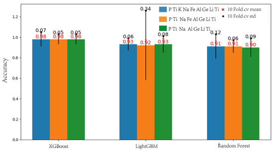
Figure 10.
Ten-fold cross-validation accuracy values of three algorithms on a dataset with different feature compositions. The red asterisks represent the mean of the ten-fold cross-validation accuracy, while the black dots represent the standard deviation of the ten-fold cross-validation accuracy.
The SHAP summary plot of the tectonic environments ranks the features in a top-down manner based on the sum of SHAP values across all individuals. Additionally, the plot illustrates the impact of the concentration of each element on the output of the classifier. The red and blue colors in the plot indicate high and low concentrations of the corresponding element for each individual, respectively. Given the good performance of the XGBoost classifier in identifying quartz, its SHAP summary plot is used as an example for analysis (Figure 11). Ti makes the greatest contribution to the discrimination of quartz from the greisen deposit (Figure 11a). In identifying quartz from epithermal deposits, high P values make the greatest contribution, while high Al values also have a certain contribution (Figure 11b). Low Ti values make the greatest contribution to the distinction of quartz in Carlin deposits, while high Al values also have a certain contribution (Figure 11c). Carlin-type gold deposits are classified as low-temperature deposits, and according to the TitaniQ geothermometer [5], they exhibit lower Ti concentrations. Furthermore, during the formation process of quartz in Carlin-type gold deposits, there exist acidic hydrothermal fluids enriched with Al ions, which enhance the absorption of Al ions by quartz crystals [71]. In the case of quartz discrimination in porphyry deposits (Figure 11d), a significant contribution is attributed to high Ti values. This is because porphyry deposits are classified as high-temperature ore deposits, and according to the TitaniQ geothermometer [5], they exhibit elevated concentrations of Ti. Discrimination of quartz in pegmatite deposits relies on high Li values (Figure 11e). This may be due to the fact that lithium content in quartz is a good indicator for predicting lithium mineralization, and there is quartz from Borborema pegmatite in the dataset, and lithium mineralization occurs in the deposit where the quartz of Borborema pegmatite is located [72]. Low P and low Ti values make a significant contribution to the discrimination of quartz in skarn deposits (Figure 11f). High Ge values, partially low Li values, and partially low P values make a significant contribution to the distinction of quartz in orogenic deposits (Figure 11g). This could be attributed to the relatively common substitution of Ge4+ for Si4+ in quartz within certain orogenic gold deposits. In distinguishing quartz in granite deposits, partially high Ti values make the greatest contribution and partially low Fe values determine the distinction of quartz in a small number of granite deposits (Figure 11h). The results presented in Figure 11 provide evidence for the distinct geochemical characteristics of quartz in different types of ore deposits, effectively explaining the variations observed in the models.
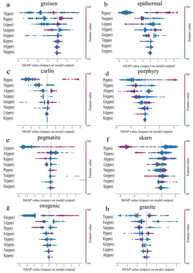
Figure 11.
A summary plot of SHAP values obtained from XGBoost for various deposits of quartz. (a) greisen. (b) epithermal. (c) carlin. (d) porphyry. (e) pegmatite. (f) skarn. (g) orogenic. (h) granite. Each point in the figure represents a sample, and the color of each point represents the concentration of elements (red = high, blue = low).
Spearman correlation is a non-parametric alternative to Pearson correlation that is more effective in handling non-linear, non-normally distributed data, and outliers. Calculating Spearman correlation coefficients between trace elements in quartz from different deposits helps uncover the relationships between these trace elements (Figure 12). Positive values in the figure indicate a positive correlation, while negative values indicate a negative correlation. In Figure 12, a strong positive correlation between Al and Li is observed in quartz. The correlation between Al and Li concentrations in quartz is documented in the literature, often attributed to the presence of trivalent Al leading to positive charge defects [73]. For most quartz samples from different ore deposits, there is no apparent correlation between Al and Ti (Figure 12a,b,c,f,g,h). This suggests that the substitution of Ti and Al for silicon ions occurs independently and may not influence each other. Similarly, Ti does not exhibit a significant correlation with other trace elements in quartz from most ore deposits (Figure 12a,b,c,f,g,h). This may be because Ti primarily occurs in the tetra-valent state and does not require charge compensation from interstitial cations. In most deposits, there is no significant correlation observed between Al and P, as well as between Ti and Ge in quartz (Figure 12a–h). This suggests that the substitution of Si4+ by Ti4+ and Ge4+ or by Al3+ and P5+ does not dominate in quartz from any deposit type. In epithermal, porphyry, and granite quartz, there is no significant correlation between Al concentration and Ge concentration, and there is no significant correlation among other elements (Fe, Na, Al, and K) (Figure 12a,d,h), which aligns with similar conclusions found in the literature [17]. In addition, in Figure 12, we also observed a positive correlation between Al and (Li, Na, and K) in the hydrothermal quartz from epithermal, orogenic gold, and porphyry deposits, as well as in quartz from granite deposits. However, the correlation between Na and Al is less pronounced (Figure 12a,d,g). This can be attributed to the fact that the Li+ concentration in quartz from these types of deposits is too low to balance the positive charge defects caused by Al3+ and other trivalent cations doping in the Si lattice. This requires compensation from other cations such as K and Na, with Li+ and K+ primarily serving as charge compensators for Al3+. In quartz from pegmatites, there is a strong positive correlation between Al, Fe, Ti, Li, Na, and K (Figure 12e). This is likely attributed to the occurrence of a single substitution of Ti4+ for Si4+ and compensatory substitutions primarily involving Al3+ and Fe3+ in pegmatitic quartz. However, neither of these substitution mechanisms dominates in abundance. As depicted in Figure 12, quartz from various ore deposits does not exhibit a strong positive correlation between P and Al or Fe. This suggests that the dual substitution of Al3+ and P5+ for Si4+ is not commonly observed in quartz. In skarn and orogenic quartz, a positive correlation is observed between Ge and Al, as well as between Ge and Li (Figure 12f,g). This positive correlation can be explained by the competitive occurrence of a single substitution of Ge4+ for Si4+ and a compensatory substitution of Al3+ for Si4+. Based on the observations above, it can be noted that despite variations in the concentrations of trace elements in most mineral deposits, there is still a general consistency in their relationships. This suggests the existence of underlying geochemical processes that control the distribution and incorporation of these trace elements into quartz, which are not strongly related to specific deposit types. These processes may involve charge compensation during hydrothermal infiltration, substitution mechanisms, and competition between elements.
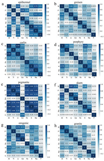
Figure 12.
A Spearman correlation heatmap of trace elements in quartz from various deposits. (a) epithermal. (b) greisen. (c) carlin. (d) porphyry. (e) pegmatite. (f) skarn. (g) orogenic. (h) granite.
5.2. Discriminant Diagram Based on Machine Learning
The binary or ternary plots used to differentiate quartz based on partial sample features are ineffective due to the insufficient feature information available. Dimensionality reduction is a valuable technique for reducing high-dimensional feature data to a lower-dimensional space, which can be used to describe and visualize the distribution of data samples. The t-distributed Stochastic Neighbor Embedding (t-SNE) algorithm is widely used for the dimensionality reduction visualization of various data due to its excellent dimensionality reduction visualization effect [40]. In this study, we propose a visualization method for a quartz classifier based on t-SNE and XGBoost (Figure 13). This process involves using t-SNE to reduce the high-dimensional feature data of quartz samples to a two-dimensional representation, followed by training an XGBoost-based classifier using this reduced data. To construct decision boundaries, a large number of equally spaced coordinates are selected on the two-dimensional plane, which is then classified using the trained classifier. Finally, the reduced quartz data are projected onto the two-dimensional plane for visualization. This approach enables us to effectively visualize the distribution of quartz samples and their classification results.
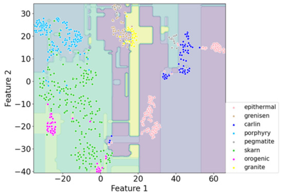
Figure 13.
A decision plane drawn using XGBoost and t-SNE.
6. Conclusions
In this study, quartz classifiers were developed based on three machine-learning algorithms: random forest, XGBoost, and LightGBM. The Shapley Additive exPlanations algorithm was applied to explain the quartz classifiers and analyze feature importance. Spearman correlation coefficients were also calculated to determine the correlations between trace elements. Additionally, the results were visualized as a two-dimensional plane using XGBoost and t-SNE to further demonstrate the effectiveness of machine-learning-based quartz classification. It was found that good performance in multiple evaluation metrics, including recall, accuracy, confusion matrix, and learning curve, was achieved by these three classifiers. In the dataset, the machine-learning-based method outperformed traditional quartz genesis classification models. The Shapley Additive exPlanations algorithm helped to better analyze the hidden relationships between trace elements and quartz formation environments. Through feature importance analysis, the ranking of influential trace elements was found to vary in different deposits. Notably, the contribution of P and Ti in distinguishing certain quartz deposits highlights the importance of these elements in the mineralization process. This study identifies the key geochemical indicators in quartz that can be used to distinguish various types of ore deposits, such as Ti in greisen and porphyry deposits, P in Carlin, skarn and epithermal deposits, Ge in orogenic deposits, and Li in greisen and skarn deposits. These trace elements can serve as useful indicators for identifying the specific type of ore deposit present in a given quartz sample. Furthermore, we conducted a detailed analysis of the impact of varying concentrations of trace elements on the identification of quartz deposits. This allowed us to determine the influence of different combinations and concentrations of trace elements on quartz identification, as well as the trends in identification results with changes in trace element content. The analysis of Spearman correlation coefficients between trace elements in quartz from various deposits revealed significant findings. A strong positive correlation was observed between Al and Li concentrations, indicating the influence of trivalent Al and positive charge effects. In various types of quartz, the substitution of Ti and Al appears to occur independently, as there is no significant correlation observed between them. In hydrothermal quartz and granite quartz, a stronger positive correlation was found between Al and elements such as Li, Na, and K. This can be attributed to low Li+ concentrations that require compensation from other cations. In skarn and orogenic ore deposits, a positive correlation is observed between Ge and Al, as well as between Ge and Li, suggesting a competitive occurrence of a single substitution of Ge4+ for Si4+ and compensatory substitutions involving Al3+ and Li+ for Si4+. The findings provided new insights into the relationships between trace elements and quartz genesis, as well as the effects of different trace element combinations and concentrations on quartz identification. It is believed that this study can contribute to the development of new methods for identifying quartz in different deposits.
Author Contributions
Conceptualization, Y.-Y.N.; writing, G.-D.Z.; review and editing, Y.-Y.N. and S.-B.L.; formal analysis, L.R., G.-D.Z. and X.-H.Z. All authors have read and agreed to the published version of the manuscript.
Funding
This work was supported by the National Natural Science Foundation of China [grant numbers 62172373, 61872325]; the Fundamental Research Funds for the Central Universities, China [grant number 2652022204].
Data Availability Statement
Data are available upon request from the Zenodo website (https://zenodo.org/record/8003079). Accessed on 1 August 2023.
Conflicts of Interest
The authors declare that they have no known competing financial interests or personal relationships that could have appeared to influence the work reported in this paper.
References
- Mao, W.; Rusk, B.; Yang, F.C.; Zhang, M.J. Physical and Chemical Evolution of the Dabaoshan Porphyry Mo Deposit, South China: Insights from Fluid Inclusions, Cathodoluminescence, and Trace Elements in Quartz. Econ. Geol. 2017, 112, 889–918. [Google Scholar] [CrossRef]
- Maydagan, L.; Fanchini, M.; Rusk, B.; Lentz, D.R.; McFarlane, C.; Impiccini, A.; Rios, F.J.; Rey, R. Porphyry to Epithermal Transition in the Altar Cu-(Au-Mo) Deposit, Argentina, Studied by Cathodoluminescence, LA-ICP-MS, and Fluid Inclusion Analysis. Econ. Geol. 2015, 110, 889–923. [Google Scholar] [CrossRef]
- Thomas, J.B.; Watson, E.B.; Spear, F.S.; Shemella, P.T.; Nayak, S.K.; Lanzirotti, A. TitaniQ under pressure: The effect of pressure and temperature on the solubility of Ti in quartz. Contrib. Mineral. Petrol. 2010, 160, 743–759. [Google Scholar] [CrossRef]
- Allan, M.M.; Yardley, B.W.D. Tracking meteoric infiltration into a magmatic-hydrothermal system: A cathodoluminescence, oxygen isotope and trace element study of quartz from Mt. Leyshon, Australia. Chem. Geol. 2007, 240, 343–360. [Google Scholar] [CrossRef]
- Wark, D.A.; Watson, E.B. TitaniQ: A titanium-in-quartz geothermometer. Contrib. Mineral. Petrol. 2006, 152, 743–754. [Google Scholar] [CrossRef]
- Kronz, A.; van den Kerkhof, A.M.; Muller, A. Analysis of low element concentrations in quartz by electron microprobe. In Quartz: Deposits, Mineralogy and Analytics; Springer: Berlin/Heidelberg, Germany, 2012; pp. 191–217. [Google Scholar] [CrossRef]
- Shah, S.A.; Shao, Y.J.; Zhang, Y.; Zhao, H.T.; Zhao, L.J. Texture and Trace Element Geochemistry of Quartz: A Review. Minerals 2022, 12, 1042. [Google Scholar] [CrossRef]
- Breiter, K.; Durisova, J.; Dosbaba, M. Quartz chemistry—A step to understanding magmatic-hydrothermal processes in ore-bearing granites: Cinovec/Zinnwald Sn-W-Li deposit, Central Europe. Ore Geol. Rev. 2017, 90, 25–35. [Google Scholar] [CrossRef]
- Götze, J. Chemistry, textures and physical properties of quartz—Geological interpretation and technical application. Mineral. Mag. 2009, 73, 645–671. [Google Scholar] [CrossRef]
- Schrön, W.; Schmädicke, E.; Thomas, R.; Schmidt, W. Geochemische Untersuchungen an Pegmatitquarzen. Z. Geol. Wiss. 1988, 16, 229–244. [Google Scholar]
- Rusk, B.J.Q.D. Cathodoluminescent textures and trace elements in hydrothermal quartz. In Quartz: Deposits, Mineralogy and Analytics; Springer: Berlin/Heidelberg, Germany, 2012; pp. 307–329. [Google Scholar] [CrossRef]
- Feng, Y.Z.; Zhang, Y.; Xie, Y.L.; Shao, Y.J.; Tan, H.J.; Li, H.B.; Lai, C.K. Ore-forming mechanism and physicochemical evolution of Gutaishan Au deposit, South China: Perspective from quartz geochemistry and fluid inclusions. Ore Geol. Rev. 2020, 119, 12. [Google Scholar] [CrossRef]
- Landtwing, M.R.; Pettke, T. Relationships between SEM-cathodoluminescence response and trace-element composition of hydrothermal vein quartz. Am. Miner. 2005, 90, 122–131. [Google Scholar] [CrossRef]
- Wang, P.; Glover, L. A tectonics test of the most commonly used geochemical discriminant diagrams and patterns. Earth-Sci. Rev. 1992, 33, 111–131. [Google Scholar] [CrossRef]
- Kempe, U.; Götze, J.; Dombon, E.; Monecke, T.; Poutivtsev, M.J.Q.D. Quartz regeneration and its use as a repository of genetic information. In Quartz: Deposits, Mineralogy and Analytics; Springer: Berlin/Heidelberg, Germany, 2012; pp. 331–355. [Google Scholar] [CrossRef]
- Wang, Y.; Qiu, K.F.; Müller, A.; Hou, Z.L.; Zhu, Z.H.; Yu, H.C. Machine Learning Prediction of Quartz Forming-Environments. J. Geophys. Res. Solid Earth 2021, 126, e2021JB021925. [Google Scholar] [CrossRef]
- Rottier, B.; Casanova, V. Trace element composition of quartz from porphyry systems: A tracer of the mineralizing fluid evolution. Miner. Depos. 2021, 56, 843–862. [Google Scholar] [CrossRef]
- Peterkova, T.; Dolejs, D. Magmatic-hydrothermal transition of Mo-W-mineralized granite-pegmatite-greisen system recorded by trace elements in quartz: Krupka district, Eastern Krusne hory/Erzgebirge. Chem. Geol. 2019, 523, 179–202. [Google Scholar] [CrossRef]
- Li, Y.E.; O’Malley, D.; Beroza, G.; Curtis, A.; Johnson, P. Machine Learning Developments and Applications in Solid-Earth Geosciences: Fad or Future? J. Geophys. Res. Solid Earth 2023, 128, 7. [Google Scholar] [CrossRef]
- Ueki, K.; Hino, H.; Kuwatani, T. Geochemical Discrimination and Characteristics of Magmatic Tectonic Settings: A Machine-Learning-Based Approach. Geochem. Geophys. Geosyst. 2018, 19, 1327–1347. [Google Scholar] [CrossRef]
- Petrelli, M.; Perugini, D. Solving petrological problems through machine learning: The study case of tectonic discrimination using geochemical and isotopic data. Contrib. Mineral. Petrol. 2016, 171, 15. [Google Scholar] [CrossRef]
- Doucet, L.S.; Tetley, M.G.; Li, Z.-X.; Liu, Y.; Gamaleldien, H. Geochemical fingerprinting of continental and oceanic basalts: A machine learning approach. Earth Sci. Rev. 2022, 233, 104192. [Google Scholar] [CrossRef]
- Zhang, P.; Zhang, Z.J.; Yang, J.; Cheng, Q.M. Machine Learning Prediction of Ore Deposit Genetic Type Using Magnetite Geochemistry. Nat. Resour. Res. 2023, 32, 99–116. [Google Scholar] [CrossRef]
- Saha, R.; Upadhyay, D.; Mishra, B. Discriminating Tectonic Setting of Igneous Rocks Using Biotite Major Element chemistry—A Machine Learning Approach. Geochem. Geophys. Geosyst. 2021, 22, 29. [Google Scholar] [CrossRef]
- Zhou, T.; Cai, Y.W.; An, M.G.; Zhou, F.; Zhi, C.L.; Sun, X.C.; Tamer, M. Visual Interpretation of Machine Learning: Genetical Classification of Apatite from Various Ore Sources. Minerals 2023, 13, 13. [Google Scholar] [CrossRef]
- Zhong, X.T.; Gallagher, B.; Liu, S.S.; Kailkhura, B.; Hiszpanski, A.; Han, T.Y.J. Explainable machine learning in materials science. NPJ Comput. Mater. 2022, 8, 19. [Google Scholar] [CrossRef]
- Lisboa, P.J.G.; Saralajew, S.; Vellido, A.; Fernandez-Domenech, R.; Villmann, T. The coming of age of interpretable and explainable machine-learning models. Neurocomputing 2023, 535, 25–39. [Google Scholar] [CrossRef]
- Selvaratnam, B.; Oliynyk, A.O.; Mar, A. Interpretable Machine Learning in Solid-State Chemistry, with Applications to Perovskites, Spinels, and Rare-Earth Intermetallics: Finding Descriptors Using Decision Trees. Inorg. Chem. 2023, 62, 10865–10875. [Google Scholar] [CrossRef] [PubMed]
- Bussmann, N.; Giudici, P.; Marinelli, D.; Papenbrock, J. Explainable Machine Learning in Credit Risk Management. Comput. Econ. 2021, 57, 203–216. [Google Scholar] [CrossRef]
- Ahmad, M.A.; Eckert, C.; Teredesai, A.; Soc, I.C. Interpretable Machine Learning in Healthcare. In Proceedings of the 6th IEEE International Conference on Healthcare Informatics (ICHI), New York, NY, USA, 4–7 June 2018; p. 447. [Google Scholar]
- Breiman, L.J.M.L. Random forests. Mach. Learn. 2001, 45, 5–32. [Google Scholar] [CrossRef]
- Li, X.M.; Zhang, Y.X.; Li, Z.K.; Zhao, X.F.; Zuo, R.G.; Xiao, F.; Zheng, Y. Discrimination of Pb-Zn deposit types using sphalerite geochemistry: New insights from machine learning algorithm. Geosci. Front. 2023, 14, 20. [Google Scholar] [CrossRef]
- Qin, B.; Huang, F.; Huang, S.C.; Python, A.; Chen, Y.F.; ZhangZhou, J. Machine Learning Investigation of Clinopyroxene Compositions to Evaluate and Predict Mantle Metasomatism Worldwide. J. Geophys. Res. Solid Earth 2022, 127, 15. [Google Scholar] [CrossRef]
- Lundberg, S.M.; Erion, G.G.; Lee, S.I. Consistent individualized feature attribution for tree ensembles. arXiv 2018, arXiv:1802.03888. [Google Scholar] [CrossRef]
- Lundberg, S.M.; Nair, B.; Vavilala, M.S.; Horibe, M.; Eisses, M.J.; Adams, T.; Liston, D.E.; Low, D.K.W.; Newman, S.F.; Kim, J.; et al. Explainable machine-learning predictions for the prevention of hypoxaemia during surgery. Nat. Biomed. Eng 2018, 2, 749–760. [Google Scholar] [CrossRef] [PubMed]
- Parsa, A.B.; Movahedi, A.; Taghipour, H.; Derrible, S.; Mohammadian, A. Toward safer highways, application of XGBoost and SHAP for real-time accident detection and feature analysis. Accid. Anal. Prev. 2020, 136, 8. [Google Scholar] [CrossRef]
- Rodriguez-Perez, R.; Bajorath, J. Interpretation of machine-learning models using shapley values: Application to compound potency and multi-target activity predictions. J. Comput. Aided Mol. Des. 2020, 34, 1013–1026. [Google Scholar] [CrossRef] [PubMed]
- Mangalathu, S.; Hwang, S.H.; Jeon, J.S. Failure mode and effects analysis of RC members based on machine-learning-based SHapley Additive exPlanations (SHAP) approach. Eng. Struct. 2020, 219, 10. [Google Scholar] [CrossRef]
- Chawla, N.V.; Bowyer, K.W.; Hall, L.O.; Kegelmeyer, W.P. SMOTE: Synthetic minority over-sampling technique. J. Artif. Intell. Res. 2002, 16, 321–357. [Google Scholar] [CrossRef]
- Van der Maaten, L.; Hinton, G. Visualizing Data using t-SNE. J. Mach. Learn. Res. 2008, 9, 2579–2605. [Google Scholar]
- Wang, Y.; Qiu, K.F.; Hou, Z.L.; Yu, H.C. Quartz Ti/Ge-P discrimination diagram: A machine learning based approach for deposit classification. Acta Petrol. Sin. 2022, 38, 281–290. [Google Scholar] [CrossRef]
- Götze, T.; Ramseyer, K. Trace Element Characteristics, Luminescence Properties and Real Structure of Quartz. In Quartz: Deposits, Mineralogy and Analytics; Götze, J., Möckel, R., Eds.; Springer: Berlin/Heidelberg, Germany, 2012; pp. 265–285. [Google Scholar]
- Breiter, K.; Svojtka, M.; Ackerman, L.; Svecova, K. Trace element composition of quartz from the Variscan Altenberg-Teplice caldera (Krusne hory/Erzgebirge Mts, Czech Republic/Germany): Insights into the volcano-plutonic complex evolution. Chem. Geol. 2012, 326, 36–50. [Google Scholar] [CrossRef]
- Breiter, K.; Badanina, E.; Durisova, J.; Dosbaba, M.; Syritso, L. Chemistry of quartz—A new insight into the origin of the Orlovka Ta-Li deposit, Eastern Transbaikalia, Russia. Lithos 2019, 348, 13. [Google Scholar] [CrossRef]
- Monnier, L.; Lach, P.; Salvi, S.; Melleton, J.; Bailly, L.; Beziat, D.; Monnier, Y.; Gouy, S. Quartz trace-element composition by LA-ICP-MS as proxy for granite differentiation, hydrothermal episodes, and related mineralization: The Beauvoir Granite (Echassieres district), France. Lithos 2018, 320, 355–377. [Google Scholar] [CrossRef]
- Pacak, K.; Zacharias, J.; Strnad, L. Trace-element chemistry of barren and ore-bearing quartz of selected Au, Au-Ag and Sb-Au deposits from the Bohemian Massif. J. Geosci. 2019, 64, 19–35. [Google Scholar] [CrossRef]
- Müller, A.; Herklotz, G.; Giegling, H. Chemistry of quartz related to the Zinnwald/Cinovec Sn-W-Li greisen-type deposit, Eastern Erzgebirge, Germany. J. Geochem. Explor. 2018, 190, 357–373. [Google Scholar] [CrossRef]
- Li, J.W.; Hu, R.Z.; Xiao, J.F.; Zhuo, Y.Z.; Yan, J.; Oyebamiji, A. Genesis of gold and antimony deposits in the Youjiang metallogenic province, SW China: Evidence from in situ oxygen isotopic and trace element compositions of quartz. Ore Geol. Rev. 2020, 116, 16. [Google Scholar] [CrossRef]
- Yan, J.; Mavrogenes, J.A.; Liu, S.; Coulson, I.M. Fluid properties and origins of the Lannigou Carlin-type gold deposit, SW China: Evidence from SHRIMP oxygen isotopes and LA-ICP-MS trace element compositions of hydrothermal quartz. J. Geochem. Explor. 2020, 215, 14. [Google Scholar] [CrossRef]
- Tanner, D.; Henley, R.W.; Mavrogenes, J.A.; Holden, P. Combining in situ isotopic, trace element and textural analyses of quartz from four magmatic-hydrothermal ore deposits. Contrib. Mineral. Petrol. 2013, 166, 1119–1142. [Google Scholar] [CrossRef]
- Feng, K. Refined Metallogenic Processes and Fluid Evolutions of Gold Deposits in the Penglai-Qixia Belt, Jiaodong. Ph.D. Thesis, University of Chinese Academy of Sciences, Beijing, China, 2020. [Google Scholar]
- Wolff, W. Microstructures and Trace Element Signatures of Orogenic Quartz Veins in the Klondike District, Yukon Territory, Canada; University of British Columbia Library: Vancouver, BC, Canada, 2012. [Google Scholar] [CrossRef]
- Beurlen, H.; Muller, A.; Silva, D.; da Silva, M.R.R. Petrogenetic significance of LA-ICP-MS trace-element data on quartz from the Borborema Pegmatite Province, northeast Brazil. Mineral. Mag. 2011, 75, 2703–2719. [Google Scholar] [CrossRef]
- Tang, H.; Zhang, H. Characteristics of Trace Elements in Quartz from No. 3 Pegmatite, Koktokay area, Xinjiang Autonomous Region, China and implication for Magmatic-Hydrothermal Evolution. Acta Mineral. Sin. 2018, 38, 15–24. [Google Scholar]
- Götze, J.; Plotze, M.; Trautmann, T. Structure and luminescence characteristics of quartz from pegmatites. Am. Miner. 2005, 90, 13–21. [Google Scholar] [CrossRef]
- Mao, W.; Zhong, H.; Zhu, W.G.; Lin, X.G.; Zhao, X.Y. Magmatic-hydrothermal evolution of the Yuanzhuding porphyry Cu-Mo deposit, South China: Insights from mica and quartz geochemistry. Ore Geol. Rev. 2018, 101, 765–784. [Google Scholar] [CrossRef]
- Xue, Q.W.; Wang, R.; Liu, S.Y.; Shi, W.X.; Tong, X.S.; Li, Y.Y.; Sun, F. Significance of chlorite hyperspectral and geochemical characteristics in exploration: A case study of the giant Qulong porphyry Cu-Mo deposit in collisional orogen, Southern Tibet. Ore Geol. Rev. 2021, 134, 104156. [Google Scholar] [CrossRef]
- Zhang, Y.; Cheng, J.M.; Tian, J.; Pan, J.; Sun, S.Q.; Zhang, L.J.; Zhang, S.T.; Chu, G.B.; Zhao, Y.J.; Lai, C. Texture and trace element geochemistry of quartz in skarn system: Perspective from Jiguanzui Cu-Au skarn deposit, Eastern China. Ore Geol. Rev. 2019, 109, 535–544. [Google Scholar] [CrossRef]
- Zhao, X.Y.; Zheng, Y.C.; Yang, Z.S.; Hu, Y. Formation and evolution of multistage ore-forming fluids in the Miocene Bangpu porphyry-skarn deposit, Southern Tibet: Insights from LA-ICP-MS trace elements of quartz and fluid inclusions. J. Asian Earth Sci. 2020, 204, 20. [Google Scholar] [CrossRef]
- Shanker, M.; Hu, M.Y.; Hung, M.S. Effect of data standardization on neural network training. Omega-Int. J. Manag. Sci. 1996, 24, 385–397. [Google Scholar] [CrossRef]
- AlShboul, R.; Thabtah, F.; Abdelhamid, N.; Al-Diabat, M. A visualization cybersecurity method based on features’ dissimilarity. Comput. Secur. 2018, 77, 289–303. [Google Scholar] [CrossRef]
- Thabtah, F.; Hammoud, S.; Kamalov, F.; Gonsalves, A.J.I.S. Data imbalance in classification: Experimental evaluation. Inf. Sci. 2020, 513, 429–441. [Google Scholar] [CrossRef]
- Vakharia, V.; Shah, M.L.; Nair, P.; Borade, H.; Sahlot, P.; Wankhede, V. Estimation of Lithium-ion Battery Discharge Capacity by Integrating Optimized Explainable-AI and Stacked LSTM Model. Batteries 2023, 9, 125. [Google Scholar] [CrossRef]
- Wang, X.Y.; Zhang, W.Y.; Zhang, W.D.; Ai, Y.B. A Machine Learning Method for Predicting Corrosion Weight Gain of Uranium and Uranium Alloys. Materials 2023, 16, 631. [Google Scholar] [CrossRef]
- Chen, T.; Guestrin, C. Xgboost: A scalable tree boosting system. In Proceedings of the 22nd ACM SIGKDD International Conference on Knowledge Discovery and Data Mining, San Francisco, CA, USA, 13–17 August 2016; pp. 785–794. [Google Scholar]
- Ke, G.L.; Meng, Q.; Finley, T.; Wang, T.F.; Chen, W.; Ma, W.D.; Ye, Q.W.; Liu, T.Y. LightGBM: A Highly Efficient Gradient Boosting Decision Tree. In Proceedings of the 31st Annual Conference on Neural Information Processing Systems (NIPS), Long Beach, CA, USA, 4–9 December 2017. [Google Scholar]
- Prechelt, L. Automatic early stopping using cross validation: Quantifying the criteria. Neural Netw. 1998, 11, 761–767. [Google Scholar] [CrossRef] [PubMed]
- Krstinic, D.; Seric, L.; Slapnicar, I. Comments on “MLCM: Multi-Label Confusion Matrix”. IEEE Access 2023, 11, 40692–40697. [Google Scholar] [CrossRef]
- Perlich, C. IBM Research Report: Learning Curves in Machine Learning; IBM: Armonk, NY, USA, 2010. [Google Scholar]
- Kumar, I.E.; Venkatasubramanian, S.; Scheidegger, C.; Friedler, S.A. Problems with Shapley-value-based explanations as feature importance measures. In Proceedings of the International Conference on Machine Learning (ICML), Online, 13–18 July 2020. [Google Scholar]
- Rusk, B.G.; Lowers, H.A.; Reed, M.H. Trace elements in hydrothermal quartz: Relationships to cathodoluminescent textures and insights into vein formation. Geology 2008, 36, 547–550. [Google Scholar] [CrossRef]
- Beurlen, H.; Thomas, R.; da Silva, M.R.R.; Muller, A.; Rhede, D.; Soares, D.R. Perspectives for Li- and Ta-Mineralization in the Borborema Pegmatite Province, NE-Brazil: A review. J. S. Am. Earth Sci. 2014, 56, 110–127. [Google Scholar] [CrossRef]
- Götze, J.; Pan, Y.M.; Müller, A. Mineralogy and mineral chemistry of quartz: A review. Mineral. Mag. 2021, 85, 639–664. [Google Scholar] [CrossRef]


Disclaimer/Publisher’s Note: The statements, opinions and data contained in all publications are solely those of the individual author(s) and contributor(s) and not of MDPI and/or the editor(s). MDPI and/or the editor(s) disclaim responsibility for any injury to people or property resulting from any ideas, methods, instructions or products referred to in the content. |
© 2023 by the authors. Licensee MDPI, Basel, Switzerland. This article is an open access article distributed under the terms and conditions of the Creative Commons Attribution (CC BY) license (https://creativecommons.org/licenses/by/4.0/).