3D Multicomponent Self-Potential Inversion: Theory and Application to the Exploration of Seafloor Massive Sulfide Deposits on Mid-Ocean Ridges

Abstract

The marine self-potential (SP) method is currently playing an increasing role in the exploration and resource evaluation of seafloor massive sulfide (SMS) deposits. SP surveys are conducted using autonomous underwater vehicles (AUV), which yield multicomponent electric field datasets. By comparing with the single-component electrical field data used to date, the inversion of these multicomponent data is expected to provide a more accurate description of the 3D structure of SMS deposits beneath the seafloor (like gradiometry in gravity surveys). We introduce an inversion algorithm specifically adapted to multicomponent SP data. A synthetic model demonstrates that the inversion of multicomponent datasets allows us to better recover the amplitude of the current density and the morphology of the ore bodies compared to using a single component of the electrical field. Next, we apply our approach to a multicomponent SP dataset collected during the DY58 oceanic cruise at the Yuhuang hydrothermal field on the Southwest Indian Ridge. Subsequently, we reconstruct the three-dimensional (3D) geometry of the SMS deposits beneath the seafloor. The AUV-based SP system with the collection of multicomponent SP data inversion appears to be a powerful tool in the exploration and evaluation of seafloor sulfide resource and, in the future, could be used in concert with induced polarization data.

1. Introduction

Seafloor massive sulfide (SMS) deposits are rich in metals such as copper, zinc, silver, and gold, which are regarded as important seafloor mineral resources for humankind [1]. These deposits can be explored and evaluated with geophysical methods. Electromagnetic methods have been broadly applied to SMS deposits. They include the magnetic method, the transient electromagnetic method, the controlled-source electromagnetic method, the direct current resistivity method, and the self-potential method [2,3,4,5,6,7,8]. The self-potential method is a passive method requiring simple equipment, including a voltmeter and a set of non-polarizing electrodes [9]. It can be easily mounted on an AUV. In recent years, the SP method has been the focus of intensive research in the context of the SMS-deposit exploration [10,11,12,13]. Meanwhile, SP can be conducted with active electromagnetic methods such as the transient electromagnetic method and/or galvanometric and induced polarization techniques [14,15,16].

SMS deposits associated with active and inactive hydrothermal systems are the setting of distinct redox reactions [17] responsible for negative self-potential anomalies just above the seafloor. Inactive hydrothermal fields characterized by the absence of water column geochemical anomalies are more mature (older) than active hydrothermal fields [18]. A silica cap is usually formed above these deposits which is, in turn, beneficial regarding the additional accumulation of sulfides leading at the end to the formation of massive sulfide deposits [19].

The use of non-polarizing (e.g., Ag/AgCl) electrodes to map the distribution of the natural electric field near the seafloor is called the marine SP method [9,20]. On shore, a reference electrode is usually located far away from the ore body, where the electric potential vanished asymptotically to zero. The potential difference between this reference electrode and the scanning electrode is generally negative over sulfide deposits [21]. For marine self-potential surveys, it is far easier to measure the potential difference between a pair of electrodes, i.e., a component of the electrical field obtained according to $E=-\nabla \phi$, where φ denotes the electrical potential (the potential difference divided by the corresponding distance between the two electrodes). Therefore, the collected data are a collection of electric field components’ time series (the analogy can be drawn to gradiometry in airborne gravity surveys [22]).

The towed marine SP surveys were mostly carried out in the early exploration phase [23,24,25]. The SP system was mounted on a deep-tow camera or transient electromagnetic systems. These types of measurements could only obtain the horizontal or the vertical component of the electrical field. These data were initially used to identify the location of the ore body and not to determine its 3D morphology [23,24,25]. The obvious disadvantage of the towed measurements is that the relative position of a pair of electrodes cannot be guaranteed to be constant (see discussion in [26]). At the same time, the cable moving in the Earth’s magnetic field may generate significant levels of noise [10], therefore reducing the signal-to-noise ratio of the recorded SP data. Recently, we took advantage of the rapid development of investigation equipment, for instance, AUV, Remotely Operate Vehicle (ROV), and Human-Occupied Vehicle (HOV). These new pieces of equipment have been used for SMS-deposit surveys [27,28,29]. Several Ag/AgCl electrodes could be mounted on AUVs in different directions, allowing for large-scale self-potential surveys [10,13], and multicomponent self-potential data could be obtained.

In order to obtain the spatial distribution of an ore body below the seafloor, the collected SP data need to be inverted. Patella (1997) [30] proposed a cross-correlation imaging method to obtain the locations of the causative sources of self-potential anomalies below the ground surface. However, the proposed method was only applicable to the case of monopolar charge aggregation. That being said, self-potential anomalies caused by redox reactions such as SMS deposits are usually dipolar in nature [31]. Revil et al. (2001) [32] extended the probability density tomography to the dipole source case, which was successfully applied to ore deposits. For instance, Kawada et al. (2018) [11] used this method at the Izena hydrothermal field of the mid–Okinawa Trough. Biswas and Sharma (2017) [33] proposed a simulated annealing algorithm for the interpretation of natural electric field data from a complex, thick slab-like model. Based on the finite element method for forward simulation, Jardani et al. (2008) [34] obtained the distribution of source current density and thus determined the flow state of the subsurface fluid by performing 3D inversion of natural potential data. They presented various deterministic and stochastic approaches useable for the SP inverse problem, sometimes based on the analogy with electroencephalographic (EEG) signals. Mendonca (2007) [35] used Green’s function to simplify the geoelectric model while considering the effects of the surrounding rock conductivity, redox potential gradient, and the conductivity of the ore body on the SP signal and finally obtained the source current density distribution by charge conservation constrained inversion. Their approach was successfully applied in the detection of a gold deposit in Peru (the Yanacocha case study).

Zhu et al. (2016) [36] used the least-squares method to invert multiple sources. Miller et al. (2018) [37] obtained the distributions of the hydrothermal fluid flow under the Tongariro volcano in New Zealand by 3D SP inversion. Zhu et al. (2020) [7] inverted the horizontal component electric field to obtain the structure of the ore body, and the 3D inversion of data was initially applied to evaluate a sulfide resource. That being said, using only a single component of the electric field is insufficient for recovering the direction and magnitude of the current density associated with the occurrence of SMS deposits below the seafloor. As depicted in Figure 1, using both the horizontal component (Ex) and vertical component (Ez) of the electric field is expected to improve the 3D characterization of SMS deposits.

In this paper, the inversion algorithm of multicomponent self-potential data is first described in detail. Our algorithm was developed thanks to the open-source framework SimPEG [38,39]. A synthetic model was performed to demonstrate that the inversion of multicomponent data yields a source model that better mimics the true shape of SMS deposits compared with the result obtain with a single component, as performed so far. Finally, the multicomponent self-potential data collected at the Yuhuang hydrothermal field (Southwest Indian Ridge) during the China DY58 cruise were inverted. The spatial distribution of the associated SMS deposits of the Yuhuang hydrothermal field was imaged in 3D.

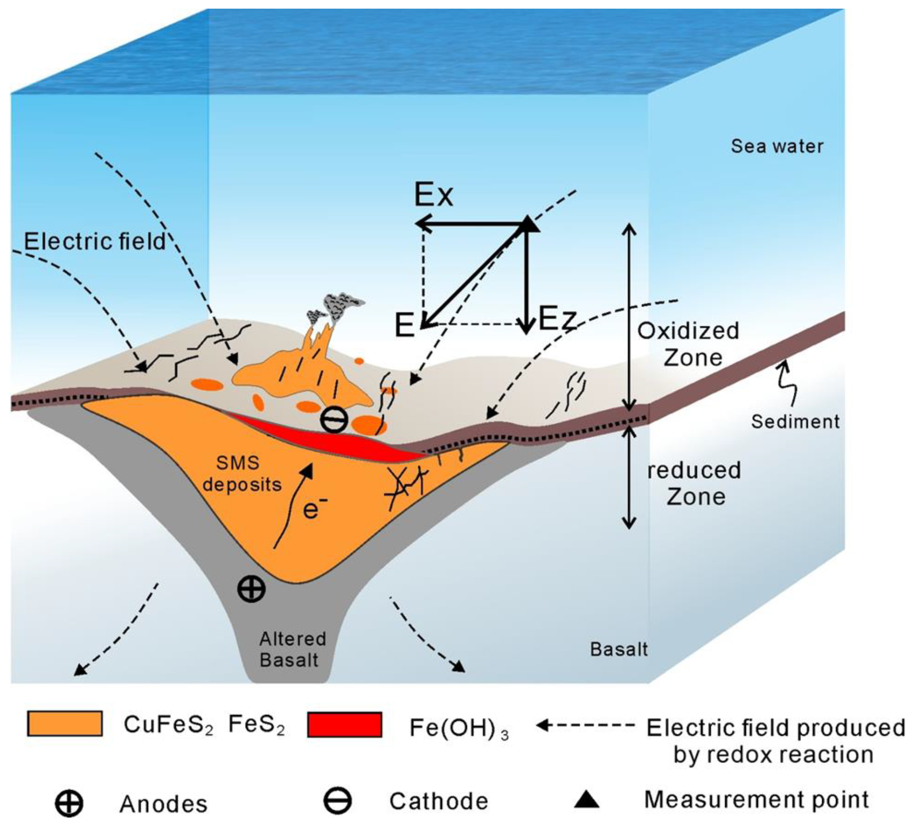
2. The Causative Source of Negative SP Anomalies above the Seafloor

We first discuss the occurrence of source current density associated with marine SMS deposits. The occurrence of a source current density associated with an ore deposit requires the presence of electron donors and electron acceptors, as well as an electronic conductor facilitating electron transport over long distances [9]. In the case of ore body corrosion, electrons are directly provided by the ore body, moving from the bottom of the ore body to the shallower part. Figure 1 provides a sketch of the redox reaction associated with an ore body. SMS deposits are rich in pyrite (FeS₂), chalcopyrite (CuFeS₂), and sphalerite (ZnS). When chalcopyrite and pyrite come into contact, chalcopyrite undergoes easier oxidation than pyrite. Consequently, chalcopyrite decomposes first, with the S (−2) in chalcopyrite being oxidized to S (0), thereby releasing Fe²⁺ and Cu²⁺ (reaction Equation (1) below). Until chalcopyrite is completely oxidized, pyrite begins to be oxidized: it releases SO₄²⁻ and Fe²⁺ (reaction Equation (2) below). The ions released by the reaction further react with the oxygen at the diving surface by flow, diffusion, and electromigration. The oxidation reaction on the surface of the deep ore body can be summarized by the following reaction equations:

$${\mathrm{CuFeS}}_2\iff {\mathrm{Cu}}^{2+}+{\mathrm{Fe}}^{2+}+\mathrm{S}+4{\mathrm{e}}^{-},$$

(1)

$${\mathrm{FeS}}_2+8{\mathrm{H}}_2\mathrm{O}\iff {\mathrm{Fe}}^{2+}+2{\mathrm{SO}}_4^{2-}{+14\mathrm{e}}^{-}{+16\mathrm{H}}^{+},$$

(2)

The half-reaction in the shallow part of the seafloor is as follows:

$$14{\mathrm{e}}^{-}+3.5{\mathrm{O}}_2+14{\mathrm{H}}^{+}\iff 7{\mathrm{H}}_2\mathrm{O},$$

(3)

$${\mathrm{Fe}}^{2+}{+\mathrm{O}}_2{+4\mathrm{H}}^{+}\iff 4{\mathrm{Fe}}^{3+}+2{\mathrm{H}}_2\mathrm{O},$$

(4)

$$4{\mathrm{Fe}}^{3+}+12{\mathrm{H}}_2\mathrm{O}\iff 4{\mathrm{Fe}\left(\mathrm{OH}\right)}_3{+12\mathrm{H}}^{+}.$$

(5)

Sato and Mooney (1960) [21] explained that the electrons are provided by other oxidation reactions, such as microbial catalysis [40,41]. In fact, the corrosion of the ore body and the oxidation reaction of other substances may exist at the same time [9], and both of them can be available to act as the anode. As a consequence, electric field anomalies are usually observed above the SMS deposits (Figure 1).

3. Forward and Inversion Methods of SP Method

3.1. Governing Equations for the Self-Potential Anomalies

The total current density, $J$, contains the conduction current density and the source current density [42],

$$J=\sigma \mathbf{E}+J_s,$$

(6)

where $\sigma$ (in S/m) denotes the conductivity below the seafloor, $E$ (V/m) denotes the quasi-static electric field, and $J_s$ (A/m²) denotes the source current density below the seafloor. The conservation of charge in the low-frequency limit of the Maxwell equations yields $\nabla \cdot j=0$ and $\mathbf{E}=-\nabla \phi$, so Equation (6) can be written as

$$\nabla \cdot \sigma \nabla \phi =\nabla \cdot J_s=q_v,$$

(7)

where $\phi$ (V) denotes the potential field, and $q_v$ (A/m³) denotes the charge density per unit volume. Moreover, Equation (7) is the govern equation of self-potential forward modeling. We discretize Equation (7) by using the finite volume method and obtain the discrete equation (see [43] for details),

$$Ku=\underset{K}{\underbrace{(\mathrm{diag}(v)D{M}_{\sigma }^{f-1}{D}^T\mathrm{diag}(v))}}\underset{u}{\underbrace{\phi }}=q_v=q_s,$$

(8)

where $K$ is the linear operator between the current density and the electrical field (kernel), $v$ is the volume of the cell, $u$ is the calculated potential filed at the cell center, $M_{\sigma }^{f-1}$ is inner product matrix (see [44] for more details), $D$ is the divergence matrix, and $q_s$ is the source term.

As we know, only a limited amount of self-potential data can be collected above the seafloor during the SP survey. Therefore, the number of observed data, ${\phi }_d$, is significantly smaller than the computational data, $\phi$, defined at the cell centers. An $N\times 3M$ interpretation matrix, $P_i$, that interpolates the field data from the computational point to the measured points is introduced. As we mentioned earlier, we used a pair of electrodes to collect potential different data above the seafloor; thus, the potential different ${\phi }_{12}$ between the electrodes can be obtained using the interpretation matrix $P=P_1-P_2$ composed of the element “±1” in each row. Finally, Equation (8) can be written as follows [45]:

$${\phi }_d=P{K}^{-1}{q}_S=P{K}^{-1}s,$$

(9)

where $s=[J_{sx}\hspace{0.17em}{J}_{sy}\hspace{0.17em}{J}_{sz}]$ describes the source term; here, $J_{sx}$, $J_{sy}$, and $J_{sz}$ represent the surface current density in the different face. Since the redox potential changes with the depth below the seafloor, the SMS deposits are regarded as the source of an electrical current density (primary source). From Equation (9), it is clear that the self-potential data, ${\phi }_d$, are related to the conductivity contrast (secondary source, the $3M\times 3M$ matrix $K$ is related to the conductivity). Therefore, it is desirable to conduct active source electromagnetic surveys to obtain the conductivity distribution below the seafloor and then carry out self-potential inversion. Indeed, combined TEM and SP data have the ability to separate primary and secondary (ghosts) source current densities in SP tomography to better image SMS deposits. This was demonstrated at the TAG Hydrothermal Mound by [16]. When the conductivity distribution below the seafloor is not known, it can be considered uniform. In this case, the calculation of the Jacobian matrix, $J$, is only related to the source current density in the model, and the process of generating the electric field by the source current density can be regarded as a linear system, and the sensitivity matrix only needs to be calculated once in the inversion, so we explicitly computed the sensitivity matrix by using the adjoint problem in this paper.

3.2. Jacobian Matrix

Combining the definition of the Jacobian matrix, $J$, with the governing equation, Equation (9), of the SP method, we obtain the Jacobian matrix as follows:

$$J=\frac{\partial {\phi }_d}{\partial s}={\left(\begin{array}{ccc}\frac{\partial {\phi }_1}{\partial s_1}& \cdot \cdot \cdot & \frac{\partial {\phi }_1}{\partial s_M}\\ ⋮& \ddots & ⋮\\ \frac{\partial {\phi }_N}{\partial s_1}& \cdots & \frac{\partial {\phi }_N}{\partial s_M}\end{array}\right)}_{N\times M}=\frac{\partial }{\partial s}(P{K}^{-1}s)=P{K}^{-1}.$$

(10)

Since the matrix $K$ is a large dense matrix, the inverse of matrix $K^{-1}$ is difficult to compute. Thus, the Jacobian matrix is not usually calculated according to Equation (10). Directly, we can solve the adjoint problem to explicitly calculate the transpose of the sensitivity matrix, $J^T=K^{-T}{P}^T$ [46]. The following shows how we can calculate the sensitivity matrix by solving the adjoint forward problem.

The matrix K is positive definite symmetric, so we have $K^{-T}=K^{-1}$. Then, the matrix $J^T$ can be expressed as

$$J^T=K^{-1}{P}^T.$$

(11)

The interpretation matrix, $P^T$, can be written as

$$P^T=(I_1,I_2,I_3,\dots ,I_N),$$

(12)

where the element “±1” is in the vector $I_N$; the location of element “1” and “−1” denotes the location of two different electrodes. Therefore, solving Equation (11) is equivalent to solving the adjoin forward equation N times,

$$K{x}_n=I_n\hspace{1em}n=1,2,\dots ,\mathrm{N}.$$

(13)

Thus, all the solutions to Equation (11) consist of $J^T=(x_1,x_2,x_3,\dots ,x_N)$.

3.3. Multicomponent SP Data Inversion

The goal of the SP inversion is to recover the current density distribution below the seafloor. To reach this goal, an objective (cost) function, $\varphi (m)$, is defined as follows:

$$\varphi \left(m\right)={\varphi }_d(m)+\beta {\varphi }_m(m)={\Vert W_d(d_{obs}-d_{pre})\Vert }_2^2+\beta {\Vert W_m(m-m_{ref})\Vert }_2^2,$$

(14)

where the regularization parameter, $\beta$, is used to balance the data misfit term (first term) and model constraint term (second term), and the optimal value of the regularization parameter is determined using the L-curve criterion (see [34,47] for details). $W_d$ is a diagonal matrix whose elements is $1/{\epsilon }_i$ (${\epsilon }_i$ denotes the standard deviation of the ith datum); $d_{obs}$ and $d_{pre}$ are the observed and predicted data, respectively; $W_m$ is the model weighting matrix; and $m$ and $m_{ref}$ represent the inversion model and the reference model, respectively. The self-potential inversion, similar in essence to other potential field techniques, such as the gravity and magnetic methods, looks to retrieve a model vector of causative current sources; the sources located close to the observation points have a lager contribution to the inversion. In order to mitigate this spurious effect, the deep or long-distance anomalies, the Jacobian matrix is normalized in such a way that the weight of the deep sources is increased. (For the construction of the depth weighting matrix, please refer to [48]). The inversion problem is a linear problem; the solution $m_{opt}$ corresponds to the minimum of the cost function (13) [9].

4. Synthetic Model Test

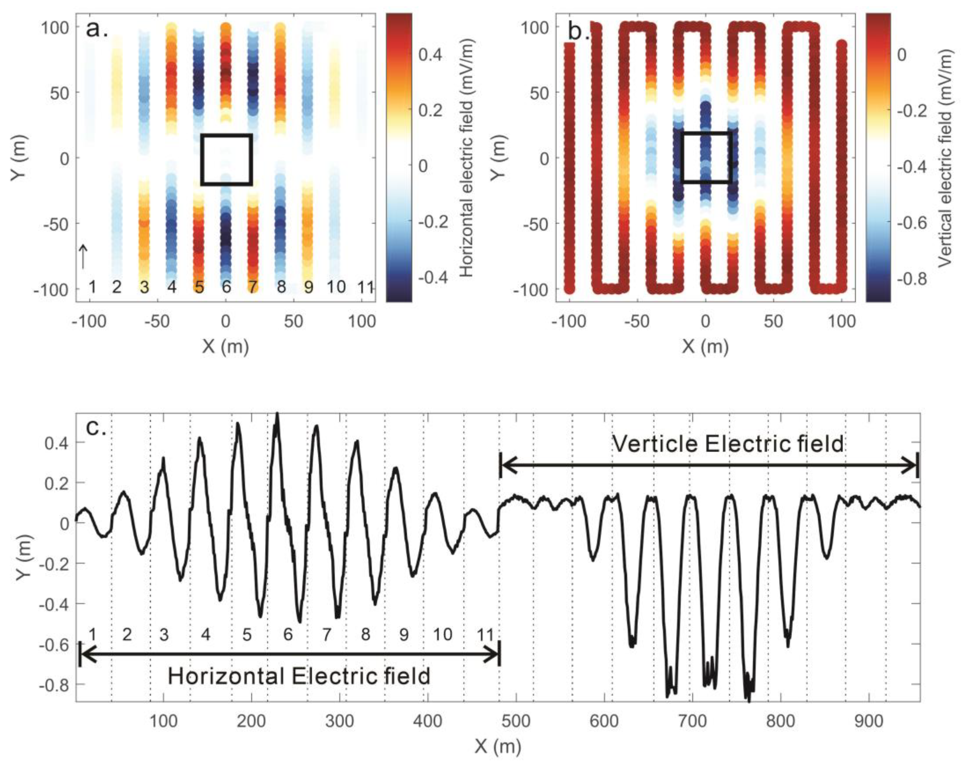
4.1. The Characteristics of Different Electric Field Components

To demonstrate the advantages of the inversion of multicomponent electric field data, we designed a simple 3D current density model (Figure 2). The mesh of the synthetic forward model shown in Figure 2 is discretized by blocks 5 × 5 × 5 m in the source volume, and the outer padding cells have an increasing width out to the boundaries of the source. The total number of meshes is 98 × 98 × 45 = 432,180. Typical SMS deposits have a shape that is similar to that shown in Figure 1 [49]. Therefore, to mimic such a shape, we use an overturned trapezoidal prism. The trapezoidal prism source volume is positioned at the center of the domain, and the vertical source current density value is set to −10 mA/m² to represent a realistic value associated with an SMS deposit. (The negative sign indicates that the direction of the current is downward, as discussed in Section 2, above.) The SMS deposit has a thickness of 40 m, extending from a depth of z = 30 m to z = −10 m. At the top, it has a maximum radius of 80 m, which gradually tapers down to a radius of 20 m at the bottom. Above the ore body, there is a cover layer with a thickness of 20 m. The source current density of the seawater and the surrounding rock below the seafloor was set to 0 mA/m².

The measurement points were set at a fixed height (30 m) above the seafloor, and the self-potential survey line is characterized by an S-shape. The distribution of the receivers is shown in Figure 2. The distance between the adjacent sampling points is 5 m. In the simulation, the horizontal and vertical component data are collected using two pairs of electrodes, and the distance of the electrode pairs is 5 m. Electrode #1 (front) and Electrode #2 (back) were used for horizontal component observation, and Electrode #3 (bottom) and Electrode #4 (up) were used for vertical observation, with the observation data arranged as a one-dimensional matrix. The observed data in Equation (2) are written as $d_{obs}={[d_{obs}^h,d_{obs}^v]}^T$, the horizontal component SP dada are $d_{obs}^h$, and the vertical component SP dada are $d_{obs}^v$. The forward responses of the different components are shown in Figure 3. The direction of the source current is downward in the ore body, and the resulting anomalous electric field is shown in Figure 1. The direction of the resulting electric field is vertical, pointing downward above the ore body, and the direction of the electric field is inclined downward around the ore body. Thus, the horizontal component of the total electric field will be reversed along the survey line, which is 0 mA/m² above the ore body (Figure 3a). The direction of the vertical component of the total electric field is always downward, so the value is the largest above the ore body, and away from the ore body, the value becomes smaller. Compared with the horizontal electric field, $d_{obs}^h$, the vertical component electric field, $d_{obs}^v$, can be used to directly delineate the boundary of the ore body.

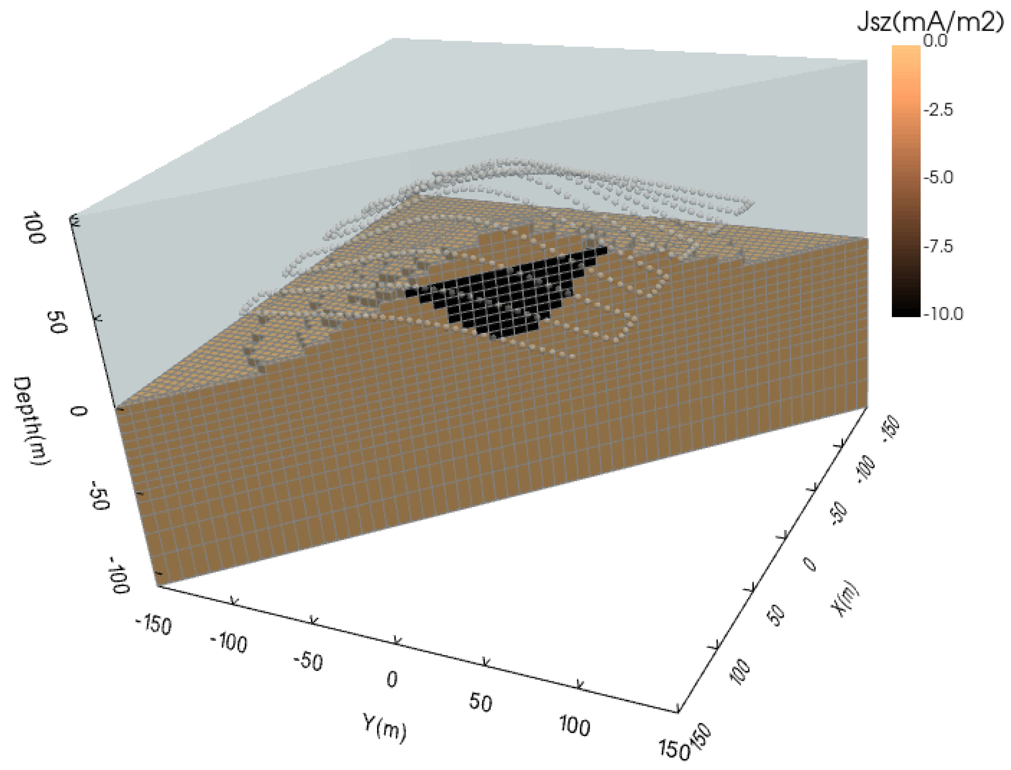
4.2. Single-Component versus Multicomponent Electric Field Results

The single-component electric field (horizontal component data) and multicomponent electric field (horizontal and vertical component data) were used to perform SP inversion. The purpose was to investigate whether the inversion results of multicomponent data can be used to obtain a more accurate spatial distribution of SMS deposits?

In the SP inversion, the regularization parameter, $\beta$, was chosen using the classical cooling strategy [50]. The value $\beta$ is equal to the estimated ratio of the largest eigenvalue of $J^{T}J$ and ${W_m}^T{W}_m$ multiply a scalar factor, to weight the relative contributions of the data misfit term and the model constraint term. In this case, the initial value of the scalar factor is set to 10 to ensure that the value of β is large enough at the beginning so that the model term dominates the data misfit term in the objection function (14). Then, we reduce the value of β until a small misfit is found [51]. The termination condition is RMS equal to 1 (here, RMS is defined as $\sqrt{\raisebox{1ex}{${\varphi }_d(m)$}\!\left/ \!\raisebox{-1ex}{$N$}\right.}$, dimensionless), or the maximum number of iterations (15) is reached.

Here, we present the inversion results for both the single-component data (Figure 4a) and multicomponent data (Figure 4b). A comparison between the two reveals that the inversion results for the multicomponent data exhibit a more focused distribution of current density, closely resembling the morphology of the ore body. Histograms of the inverted current density are shown in Figure 4c (single-component data) and Figure 4d (multicomponent data). It is evident from these histograms that the anomalies obtained via the inversion of the multicomponent data are closer to the true model (−10 mA/m²). Furthermore, the predicted data obtained from both inversions show a good fit with the observed electric field values (Figure 4e,f). Consequently, the inversion results based on the synthetic 3D model show that the inversion of multicomponent data can better recover the structure of SMS deposits.

4.3. Comparing the Computation Times and Memory for the Different Inversion

Both SP inversions were implemented on the PC computer equipped with an Intel Core i7-7820HQ 2.90 GHz CPU.

Table 1. Comparison of the different types of data used for the SP inversion.

Data for Inversion	Number of Data	Mesh	Time (min)	Memory (MB)	Iterations
Ex	479	90 × 90 × 43	12.19	561	10
Ex + Ez	958	90 × 90 × 43	17.23	615	10

illustrates a comparison of the time and memory usage for the different inversions. Both inversions used the same mesh, but the multicomponent data consisted of twice as many data points as the single-component data. Although the memory usage was similar for both cases, the inversion for the multicomponent data took longer to complete.

5. Field Data Application

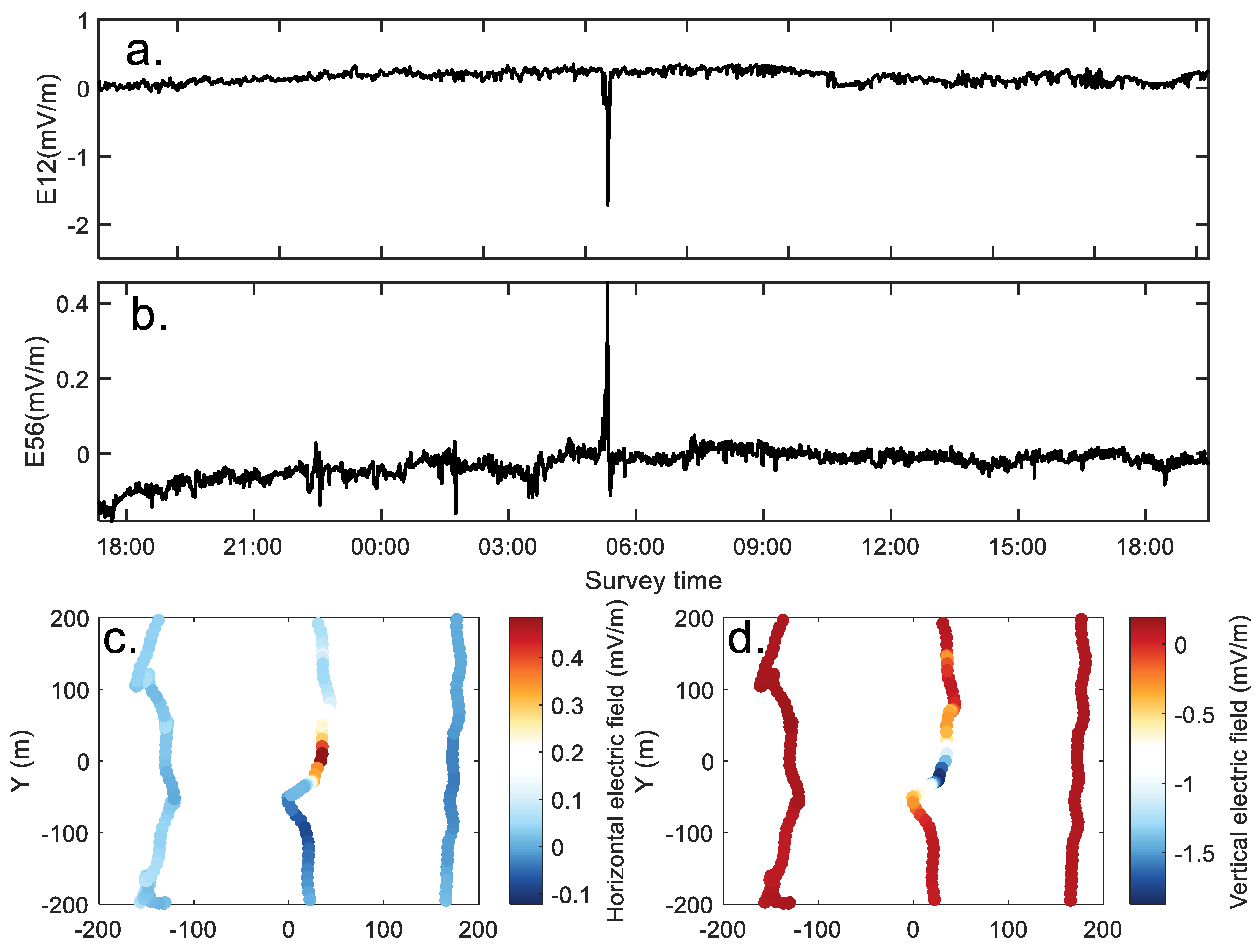
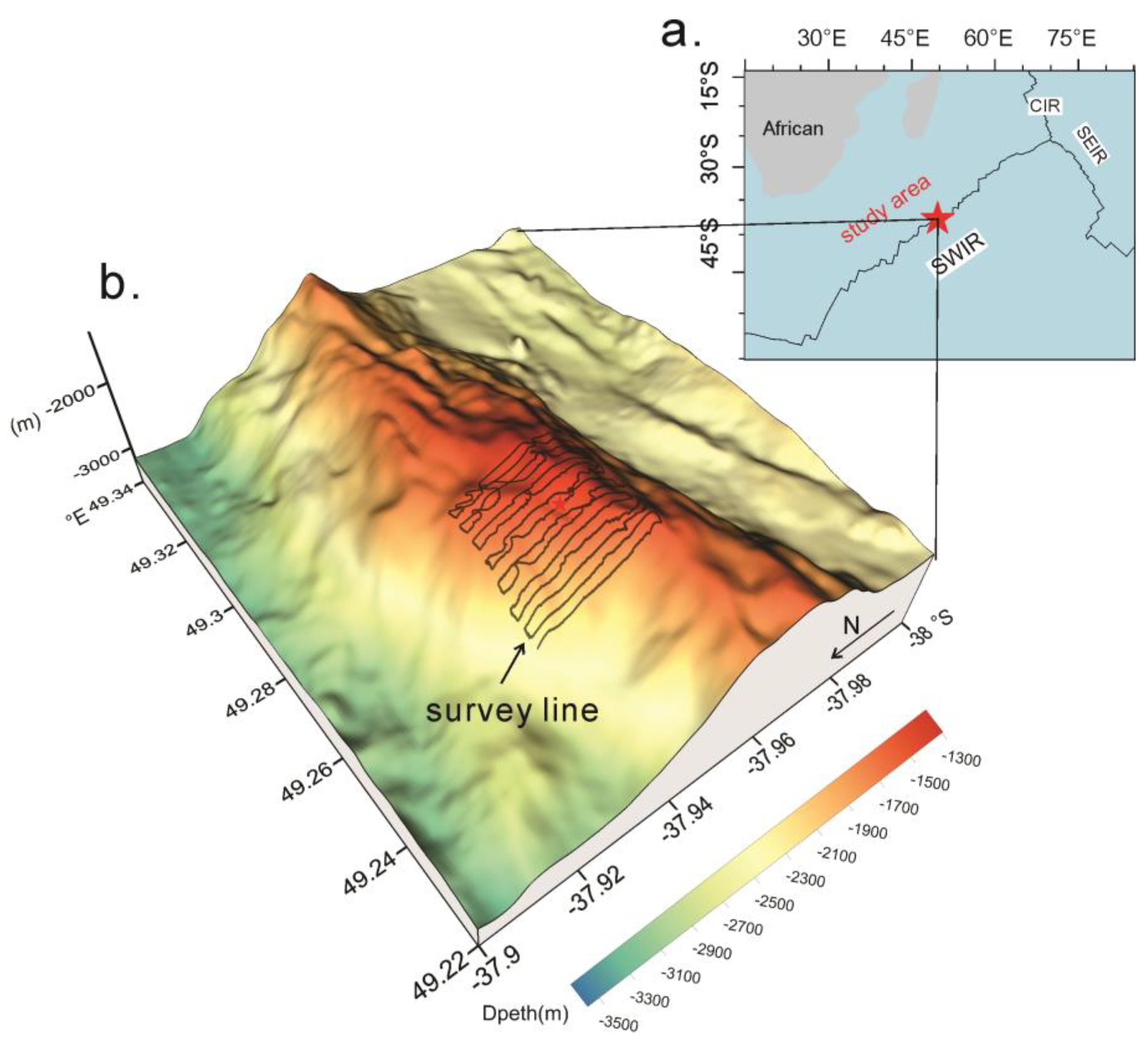
5.1. Data Acquisition

We now recount how we applied our methodology to a real case study. For this purpose, we used the multicomponent electric field collected at Yuhuang hydrothermal field on Southwest Indian ridge during the Research DY58 cruise in 2020. Six Ag/AgCl non-polarized electrodes were mounted on the Qianlong II AUV (Figure 5a). The speed of the AUV was 0.5–1.0 m/s, and the AUV was maintained at an average altitude of ~50 m above the seafloor.

The recorded SP survey line is reported in Figure 5b. Three pairs of non-polarized electrodes (channels 1–6) were used to measure the potential differences: ${\phi }_{12}(={\phi }_1-{\phi }_2)$, ${\phi }_{34}(={\phi }_3-{\phi }_4)$, and ${\phi }_{56}(={\phi }_5-{\phi }_6)$. The position of the electrodes is shown in Figure 6. From the potential differences and the distance between the electrodes, we determined the electric field, E, along the measurement survey. Two horizontal components (E₃₄, E₅₆) and one vertical component electric field (E₁₂) were simultaneously collected, and their combination can be used to assess the electrical field in regard to both amplitude and direction. The distance of Electrodes #1 and #2 is 1 m, the distance of Electrode #3 and #4 is 3.5 m (first horizontal component), and E₅₆ (the second horizontal component) is characterized by a spacing of 1.2 m. Compared to Electrodes #3 and #4, which collected the data E₃₄, the electrode dipole consisting of Electrodes #5 and #6 is located far away from the body of the AUV itself; therefore, the signal-to-noise ratio of the electric field E₅₆ is higher than it is for the other components. At the same time, the E₃₄ and E₅₆ are both part of the horizontal electric field. Therefore, the data processing and analysis in horizontal and vertical directions were focused on the horizontal electric field E₅₆ (Figure 7c) and vertical E₁₂ (Figure 7d).

5.2. Data Processing

The data from the attitude sensors on the AUV showed that the attitude of the AUV was relatively stable above the seafloor during the SP survey, with the pitch angle roughly within ±10° and the angle of cross roll controlled within ±3° [13]. The source of noise in horizontal component data E₅₆ and vertical component data E₁₂ is different. The noise in the data E₅₆ comes from the drift and variable temperature. For the data E₁₂, the distance of Electrodes #1 and #2 is short (approximately 1 m), and they are closer to the propellers, so the noise of the vertical component is mainly from the AUV propellers’ rotation. Su et al. [13] showed the denoising flow of horizontal component data E₅₆; here, we first used the same procedure to process the vertical component data E₁₂. Then, the corrected vertical component data eliminated the noise introduced by the motor rotation. The corrected and filtered vertical component (E₁₂) and corrected horizontal component (E₅₆) electric field data displayed in Figure 7a,b were obtained, and the consistent anomalous appeared in the horizontal and vertical components’ data at ~GMT 6:00 (where the maximum value of the horizontal component reaches 0.5 mV/m and the maximum value of the vertical component is about −1.8 mV/m. We matched the data with the ultra-short baseline (USBL) data on the AUV, and the 2D horizontal and vertical electric field data used to invert are shown in Figure 7c,d. As for the inversion of multicomponent data in the synthetic model test, the different components were rearranged (i.e., the horizontal component is in the first place, and the vertical component follows behind).

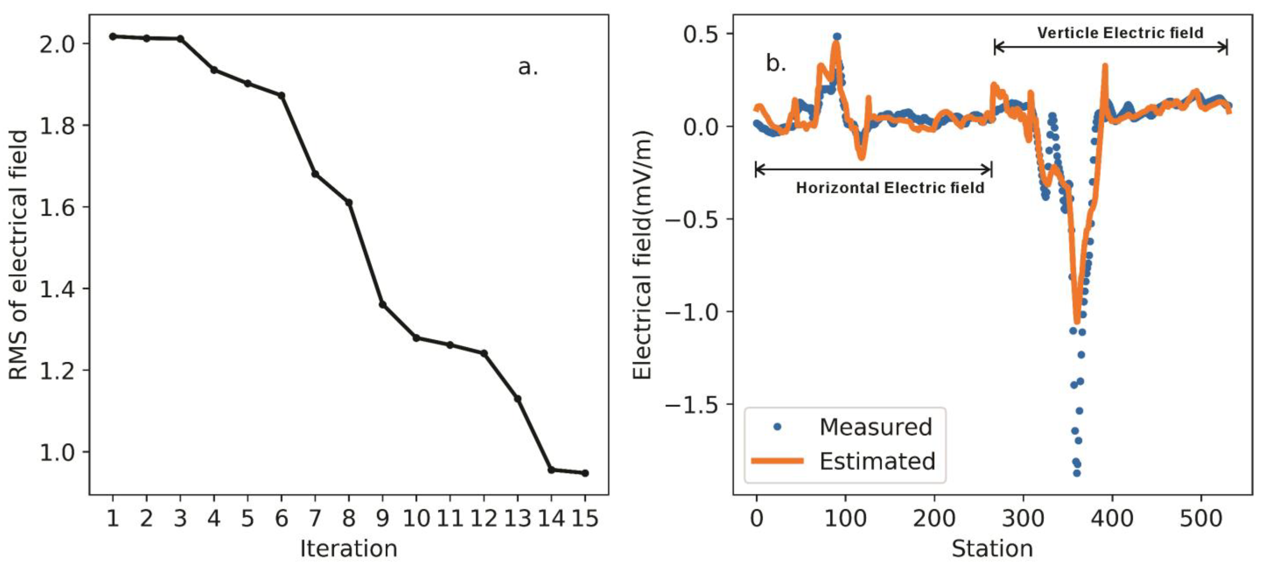
5.3. Inversion Results of Multicomponent Data

The 3D inversion of the horizontal and vertical electric field data was performed to obtain the geometry of SMS deposits at the Yuhuang hydrothermal field. A value of 0.1 S/m was chosen as the conductivity of the surrounding rocks below the seafloor based on measurements of laboratory rocks’ electrical properties [7]. The in situ conductivity of the seawater was measured by CTD sensors (average conductivity at 3.2 S/m during the survey). The seawater and base rock below the seafloor were dissected with a 3D tensor mesh. In the core area of the SP anomaly, the fine mesh has a cell size of 10 × 10 × 5 m, and the outer padding cells have an increasing width that extends out to the boundaries of the model. There are 532 observations data in the inversion. The observation noise is set to be 5% and the maximum number of iterations is 15 (Figure 8a). The measured electric field and the predicted electric field are shown in Figure 8b. We note that the measured electric field is well reproduced by the inverted source current density distribution.

The inverted 3D current density is shown in Figure 9a. Three compact negative-current sources that are associated with ore bodies below the seafloor were recovered. The largest current anomaly extends 80 m below the seafloor, which shows to be about 100 m long in the north–south direction and 100 m long in the east–west direction, and it corresponds well with the previous geological survey (Figure 9b). The fine geometry of the ore was mapped, and we provide key elements for resource evaluation.

6. Conclusions

Usually, the inversion of self-potential data near the seafloor for the localization and source current density inversion is performed with the measurement of a single component of the electrical field. A synthetic model test was first used to quantify how the inversion results of multicomponent data can better recover the distribution and amplitude of the source current density caused by ore bodies. Then, our 3D inversion approach was applied to a multicomponent self-potential dataset collected at the Yuhuang hydrothermal field during the Research DY58 oceanic cruise. We obtained the spatial distribution of ore bodies by inverting for the source current density distribution. The advantage of the AUV-based self-potential method is that it overcomes the influence of the seafloor currents in order to stabilize the position of the electrodes along a smooth path. In addition, the simultaneous acquisition of multicomponent self-potential data represents an advantage since this additional information can effectively be used to better image ore bodies.

The AUV-based SP method and 3D inversion of multicomponent data are expected to play an important role in the future exploration and resource evaluation of SMS deposits. However, current collection methods of SP data have drawbacks. The electrodes are too close to the propeller of the AUV, and the collected signals are subject to electromagnetic interference from the AUV, so we need to make sure that the electrodes are far away from the AUV to further improve the signal-to-noise ratio of the data. Such an approach will also be valuable in collected induced-polarization data that could be used in concert with SP data in order to improve SMS-deposit imaging.

References

1. Hannington, M.; Jamieson, J.; Monecke, T.; Petersen, S.; Beaulieu, S. The abundance of seafloor massive sulfide deposits. Geology 2011, 39, 1155–1158. [Google Scholar] [CrossRef]
2. Müller, H.; Schwalenberg, K.; Reeck, K.; Barckhausen, U.; Schwarz-Schampera, U.; Hilgenfeldt, C.; von Dobeneck, T. Mapping seafloor massive sulfides with the Golden Eye frequency-domain EM profiler. First Break 2018, 36, 61–67. [Google Scholar] [CrossRef]
3. Ishizu, K.; Goto, T.; Ohta, Y.; Kasaya, T.; Iwamoto, H.; Vachiratienchai, C.; Siripunvaraporn, W.; Tsuji, T.; Kumagai, H.; Koike, K. Internal structure of a seafloor massive sulfide deposit by electrical resistivity tomography, Okinawa Trough. Geophys. Res. Lett. 2019, 46, 11025–11034. [Google Scholar] [CrossRef]
4. Galley, C.; Lelièvre, P.; Haroon, A.; Graber, S.; Jamieson, J.; Szitkar, F.; Yeo, I.; Farquharson, C.; Petersen, S.; Evans, R. Magnetic and Gravity Surface Geometry Inverse Modeling of the TAG Active Mound. J. Geophys. Res. Solid Earth 2021, 126, e22228. [Google Scholar] [CrossRef]
5. Haroon, A.; Hölz, S.; Gehrmann, R.A.S.; Attias, E.; Jegen, M.; Minshull, T.A.; Murton, B.J. Marine dipole-dipole controlled source electromagnetic and coincident-loop transient electromagnetic experiments to detect seafloor massive sulphides: Effects of three-dimensional bathymetry. Geophys. J. Int. 2018, 215, 2156–2171. [Google Scholar] [CrossRef]
6. Gehrmann, R.; North, L.J.; Graber, S.; Szitkar, F.; Petersen, S.; Minshull, T.; Murton, B. Marine mineral exploration with controlled source electromagnetics at the TAG hydrothermal field, 26° N Mid-Atlantic Ridge. Geophys. Res. Lett. 2019, 46, 5808–5816. [Google Scholar] [CrossRef]
7. Zhu, Z.; Tao, C.; Shen, J.; Revil, A.; Deng, X.; Liao, S.; Zhou, J.; Wang, W.; Nie, Z.; Yu, J. Self-potential tomography of a deep-sea polymetallic sulfide deposit on Southwest Indian Ridge. J. Geophys. Res. Solid Earth 2020, 125, e2020JB019738. [Google Scholar] [CrossRef]
8. Ishizu, K.; Siripunvaraporn, W.; Goto, T.-N.; Koike, K.; Kasaya, T.; Iwamoto, H. A cost-effective three-dimensional marine controlled-source electromagnetic survey: Exploring seafloor massive sulfides. Geophysics 2022, 87, E219–E241. [Google Scholar] [CrossRef]
9. Revil, A.; Jardani, A. The Self-Potential Method: Theory and Applications in Environmental Geosciences; Cambridge University Press: Cambridge, UK, 2013. [Google Scholar]
10. Constable, S.; Kowalczyk, P.; Bloomer, S. Measuring marine self-potential using an autonomous underwater vehicle. Geophys. J. Int. 2018, 215, 49–60. [Google Scholar] [CrossRef]
11. Kawada, Y.; Kasaya, T. Self-potential mapping using an autonomous underwater vehicle for the Sunrise deposit, Izu-Ogasawara arc, southern Japan. Earth Planets Space 2018, 70, 142. [Google Scholar] [CrossRef]
12. Szitkar, F.; Hölz, S.; Tarits, P.; Petersen, S. Deep-Sea Electric and Magnetic Surveys Over Active and Inactive Basalt-Hosted Hydrothermal Sites of the TAG Segment (26°, MAR): An Optimal Combination for Seafloor Massive Sulfide Exploration. J. Geophys. Res. Solid Earth 2021, 126, e2021JB022082. [Google Scholar] [CrossRef]
13. Su, Z.; Tao, C.; Shen, J.; Revil, A.; Zhu, Z.; Deng, X.; Nie, Z.; Li, Q.; Liu, L.; Wu, T. 3D self-potential tomography of seafloor massive sulfide deposits using an autonomous underwater vehicle. Geophysics 2022, 87, B255–B267. [Google Scholar] [CrossRef]
14. Revil, A.; Karaoulis, M.; Srivastava, S.; Byrdina, S. Thermoelectric self-potential and resistivity data localize the burning front of underground coal fires. Geophysics 2013, 78, B259–B273. [Google Scholar] [CrossRef]
15. Kasaya, T.; Iwamoto, H.; Kawada, Y.; Hyakudome, T.J.T. Marine DC resistivity and self-potential survey in the hydrothermal deposit areas using multiple AUVs and ASV. TAO Terr. Atmos. Ocean. Sci. 2020, 31, 579–588. [Google Scholar] [CrossRef]
16. Su, Z.; Tao, C.; Zhu, Z.; Revil, A.; Shen, J.; Nie, Z.; Li, Q.; Deng, X.; Zhou, J.; Liu, L. Joint Interpretation of Marine Self-Potential and Transient Electromagnetic Survey for Seafloor Massive Sulfide (SMS) Deposits: Application at TAG Hydrothermal Mound, Mid-Atlantic Ridge. J. Geophys. Res. Solid Earth 2022, 127, e2022JB024496. [Google Scholar] [CrossRef]
17. Yamamoto, M.; Nakamura, R.; Takai, K. Deep-sea hydrothermal fields as natural power plants. ChemElectroChem 2018, 5, 2162–2166. [Google Scholar] [CrossRef]
18. Petersen, S.; Krätschell, A.; Augustin, N.; Jamieson, J.; Hein, J.R.; Hannington, M.D.J.M.P. News from the seabed—Geological characteristics and resource potential of deep-sea mineral resources. Mar. Policy 2016, 70, 175–187. [Google Scholar] [CrossRef]
19. Murton, B.J.; Lehrmann, B.; Dutrieux, A.M.; Martins, S.; de la Iglesia, A.G.; Stobbs, I.J.; Barriga, F.J.; Bialas, J.; Dannowski, A.; Vardy, M.E. Geological fate of seafloor massive sulphides at the TAG hydrothermal field (Mid-Atlantic Ridge). Ore Geol. Rev. 2019, 107, 903–925. [Google Scholar] [CrossRef]
20. Nyquist, J.E.; Corry, C.E. Self-potential: The ugly duckling of environmental geophysics. Lead. Edge 2002, 21, 446–451. [Google Scholar] [CrossRef]
21. Sato, M.; Mooney, H.M. The electrochemical mechanism of sulfide self-potentials. Geophysics 1960, 25, 226–249. [Google Scholar] [CrossRef]
22. Jekeli, C. A review of gravity gradiometer survey system data analyses. Geophysics 1993, 58, 508–514. [Google Scholar] [CrossRef]
23. Corwin, R.F.; Hoover, D.B. The self-potential method in geothermal exploration. Geophysics 1979, 44, 226–245. [Google Scholar] [CrossRef]
24. Kawada, Y.; Kasaya, T. Marine self-potential survey for exploring seafloor hydrothermal ore deposits. Sci. Rep. 2017, 7, 13552. [Google Scholar] [CrossRef] [PubMed]
25. Sudarikov, S.M.; Roumiantsev, A.B. Structure of hydrothermal plumes at the Logatchev vent field, 14°45′ N, Mid-Atlantic Ridge: Evidence from geochemical and geophysical data. J. Volcanol. Geotherm. Res. 2000, 101, 245–252. [Google Scholar] [CrossRef]
26. Zhu, Z.; Shen, J.; Tao, C.; Deng, X.; Wu, T.; Nie, Z.; Wang, W.; Su, Z. Autonomous-underwater-vehicle-based marine multicomponent self-potential method: Observation scheme and navigational correction. Geosci. Instrum. Methods Data Syst. 2021, 10, 35–43. [Google Scholar] [CrossRef]
27. MacGregor, L.; Kowalczyk, P.; Galley, C.; Weitemeyer, K.; Bloomer, S.; Phillips, N.; Proctor, A. Characterization of Seafloor Mineral Deposits Using Multiphysics Datasets Acquired from an AUV. First Break 2021, 39, 63–69. [Google Scholar] [CrossRef]
28. Okamoto, A.; Seta, T.; Sasano, M.; Inoue, S.; Ura, T. Visual and Autonomous Survey of Hydrothermal Vents Using a Hovering-Type AUV: Launching Hobalin Into the Western Offshore of Kumejima Island. Geochem. Geophys. Geosyst. 2019, 20, 6234–6243. [Google Scholar] [CrossRef]
29. García, M.; Dowdeswell, J.A.; Noormets, R.; Hogan, K.; Evans, J.; Cofaigh, C.Ó.; Larter, R.D. Geomorphic and shallow-acoustic investigation of an Antarctic Peninsula fjord system using high-resolution ROV and shipboard geophysical observations: Ice dynamics and behaviour since the Last Glacial Maximum. Quat. Sci. Rev. 2016, 153, 122–138. [Google Scholar] [CrossRef]
30. Patella, D. Self-potential global tomography including topographic effects. Geophys. Prospect. 1997, 45, 843–863. [Google Scholar] [CrossRef]
31. Chou, Y. Spatial distribution of spontaneous potential of metallic orebody and its application. Geophys. Geochem. Explor. 1985, 9, 268–273. (In Chinese) [Google Scholar]
32. Revil, A.; Ehouarne, L.; Thyreault, E. Tomography of self-potential anomalies of electrochemical nature. Geophys. Res. Lett. 2001, 28, 4363–4366. [Google Scholar] [CrossRef]
33. Biswas, A.; Sharma, S.P. Interpretation of self-potential anomaly over 2-D inclined thick sheet structures and analysis of uncertainty using very fast simulated annealing global optimization. Acta Geod. Geophys. 2017, 52, 439–455. [Google Scholar] [CrossRef]
34. Jardani, A.; Revil, A.; Bolève, A.; Dupont, J.P. Three-dimensional inversion of self-potential data used to constrain the pattern of groundwater flow in geothermal fields. J. Geophys. Res. Solid Earth 2008, 113, B9. [Google Scholar] [CrossRef]
35. Mendonça, C.A. Forward and inverse self-potential modeling in mineral exploration. Geophysics 2007, 73, F33–F43. [Google Scholar] [CrossRef]
36. Zhu, X.; Cui, Y.; Chen, Z. Inversion for self-potential sources based on the least squares regularization. Prog. Geophys. 2016, 31, 2313. (In Chinese) [Google Scholar]
37. Miller, C.A.; Kang, S.; Fournier, D.; Hill, G. Distribution of vapor and condensate in a hydrothermal system: Insights from self-potential inversion at Mount Tongariro, New Zealand. Geophys. Res. Lett. 2018, 45, 8190–8198. [Google Scholar] [CrossRef]
38. Cockett, R.; Kang, S.; Heagy, L.J.; Pidlisecky, A.; Oldenburg, D.W. SimPEG: An open source framework for simulation and gradient based parameter estimation in geophysical applications. Comput. Geosci. 2015, 85, 142–154. [Google Scholar] [CrossRef]
39. Heagy, L.J.; Cockett, R.; Kang, S.; Rosenkjaer, G.K.; Oldenburg, D.W. A framework for simulation and inversion in electromagnetics. Comput. Geosci. 2017, 107, 1–19. [Google Scholar] [CrossRef]
40. Revil, A.; Vaudelet, P.; Su, Z.; Chen, R. Induced Polarization as a Tool to Assess Mineral Deposits: A Review. Minerals 2022, 12, 571. [Google Scholar] [CrossRef]
41. Revil, A.; Su, Z.; Zhu, Z.; Maineult, A. Self-Potential as a Tool to Monitor Redox Reactions at an Ore Body: A Sandbox Experiment. Minerals 2023, 13, 716. [Google Scholar] [CrossRef]
42. Sill, W.R. Self-potential modeling from primary flows. Geophysics 1983, 48, 76–86. [Google Scholar] [CrossRef]
43. Cockett, R.; Heagy, L.J.; Oldenburg, D.W. Pixels and their neighbors: Finite volume. Lead. Edge 2016, 35, 703–706. [Google Scholar] [CrossRef]
44. Haber, E. Computational Methods in Geophysical Electromagnetics; Mathematics in Industry; Society for Industrial and Applied Mathematics: Philadelphia, PA, USA, 2014. [Google Scholar]
45. Minsley, B.J.; Sogade, J.; Morgan, F.D. Three-dimensional source inversion of self-potential data. J. Geophys. Res. 2007, 112, B2. [Google Scholar] [CrossRef]
46. Liu, Y.; Yin, C.; Qiu, C.; Hui, Z.; Zhang, B.; Ren, X.; Weng, A. 3-D inversion of transient EM data with topography using unstructured tetrahedral grids. Geophys. J. Int. 2019, 217, 301–318. [Google Scholar] [CrossRef]
47. Hansen, P.C.; O’Leary, D.P. The Use of the L-Curve in the Regularization of Discrete Ill-Posed Problems. SIAM J. Sci. Comput. 1993, 14, 1487–1503. (In English) [Google Scholar] [CrossRef]
48. Spinelli, L. Analyse Spatiale de L’activité Electrique Cérébrale: Nouveaux Développements. Ph.D. Thesis, Université Joseph-Fourier-Grenoble I, Grenoble, France, 1999. [Google Scholar]
49. Hannington, M.D.; Galley, A.G.; Herzig, P.M.; Petersen, S. Comparison of the TAG mound and stockwork complex with Cyprus-type massive sulfide deposits. Oceanogr. Lit. Rev. 1998, 158, 1557–1558. [Google Scholar]
50. Nocedal, J.; Wright, S.J. Numerical Optimization; Springer: Berlin/Heidelberg, Germany, 1999. [Google Scholar]
51. Oldenburg, D.W.; Li, Y.J.N.-S.G. Inversion for applied geophysics: A tutorial. Near-Surf. Geophys. 2005, 89–150. [Google Scholar]
Figure 1. Sketch of the geo-battery model associated with a massive ore body at a hydrothermal field. The redox reactions occur at the surface of the ore body, and the distribution of the gradient of the redox potential drives the flow of charge carriers inside the ore body, so electrical field anomalies are established that are associated with this current density (modified from [7,9,21]).
Minerals 13 01098 g001
Figure 2. Three-dimensional current density model, where the gray dots indicate the location of the survey line, and the black trapezoidal prism anomalies indicate the ore body (the magnitude of current density of ore body is −10 mA/m2, the minus sign means the natural current flow downward, and the background value is set to 0 mV/m2).
Minerals 13 01098 g002
Figure 3. The characteristics of synthetical horizontal and vertical components’ electric field. (a) Two-dimensional map (a slice at depth of 0 m) of horizontal component electric field distribution; the black rectangle indicates the location of the ore body. The black arrow indicates the direction of the survey line, and the number indicates the survey line. (b) Two-dimensional plane map of vertical component electric field. (c) One-dimensional multicomponent electric field data used for self-potential inversion.
Minerals 13 01098 g003
Figure 4. The 3D inversion results of the synthetic model and the fitting curve between the predicted data and the observed data. (a) Inversion results of single-component data; the white trapezoid represents the boundary of the ore body. (b) Inversion results of multicomponent data. (c) The density distribution histogram was obtained by single-component self-potential data inversion (orange line represents true current density; blue line represents inverted current density). (d) The density distribution histogram obtained by single-component self-potential data inversion (orange line represents true current density; blue line represents inverted current density). (e) Measured electric field versus the estimated electric field for the last iteration when convergence is reached. (f) Measured electric field versus the estimated electric field for the last iteration when convergence is reached.
Minerals 13 01098 g004
Figure 5. Bathymetry and AUV-based self-potential survey lines of Yuhuang hydrothermal field: (a) Bathymetry of Yuhuang hydrothermal area obtained by ship-borne multi-beam and (b) self-potential survey lines (red dots indicate the location of the Yuhuang hydrothermal field).
Minerals 13 01098 g005
Figure 6. Schematic diagram of AUV-based self-potential system. The numbers on the AUV show the locations of six Ag/AgCl electrodes. Electrodes #1 and #2 were used to measure the vertical electric field E12, Electrodes #3 and #4 were used to measure the horizontal electric field E34, and Electrodes #5 and #6 were used to measure the horizontal electric field E56. The CTD sensor mounted on the AUV was used to measure in the situ conductivity and temperature of seawater along the survey.
Minerals 13 01098 g006
Figure 7. Corrected vertical and horizontal component electric field data. (a) Vertical component data E12 after filtering and collection. (b) Horizontal component data E56 after filtering and collection. (c) Two-dimensional distribution of horizontal component data E56 and (d) 2D distribution of vertical component data E12.
Minerals 13 01098 g007
Figure 8. Convergence of the inversion algorithm and fitted data of multicomponent SP inversion. (a) The RMS of the data misfit versus the number of iterations used to minimize the cost function. (b) Fitting curve of estimated data (the orange line) for the last iteration and measured data (the blue dots).
Minerals 13 01098 g008
Figure 9. Inversion result of the multicomponent SP data. (a) The red-colored volumes denote the inverted negative-source current densities. In turn, these anomalies represent the polymetallic sulfide deposits. (b) Geometry of polymetallic sulfide ore bodies on the seafloor (current densities in the range from −0.5 mA/m2 to −0.15 mA/m2). The gray surface underlines the position of the seafloor.
Minerals 13 01098 g009