Article

Low-Dimensional Multi-Trace Impedance Inversion in Sparse Space with Elastic Half Norm Constraint

1
National Key Laboratory of Deep Oil and Gas, China University of Petroleum (East China), Qingdao 266580, China
2
China National Offshore Oil Corporation (CNOOC) Limited Tianjin Branch, Tianjin 300450, China
3
Changqing Geophysical Department, BGP Inc., China National Petroleum Corporation, Xi’an 710021, China
*
Author to whom correspondence should be addressed.
Minerals 2023, 13(7), 972; https://doi.org/10.3390/min13070972
Submission received: 25 May 2023 / Revised: 18 July 2023 / Accepted: 20 July 2023 / Published: 22 July 2023

Abstract

:
Recently, multi-trace impedance inversion has attracted great interest in seismic exploration because it improves the horizontal continuity and fidelity of the inversion results by exploiting the lateral structure information of the strata. However, computational inefficiency affects its practical application. Furthermore, in terms of vertical constraints on the model parameters, it only considers smooth features while ignoring sharp discontinuity features. This leads to yielding an over-smooth solution that does not accurately reflect the distribution of underground rock. To deal with the above situations, we first develop a low-dimensional multi-trace impedance inversion (LMII) framework. Inspired by compressed sensing, this framework utilizes low-dimensional measurements in sparse space containing the maximum information of the signal to construct the objective function for multi-trace inversion, which can significantly reduce the size of the inversion problem and improve the inverse efficiency. Then, we introduce the elastic half (EH) norm as a vertical constraint on the model parameters in the LMII framework and formulate a novel constrained LMII model for impedance inversion. Because the introduced EH norm takes into account both the smoothness and blockiness of rock impedance, the constrained LMII model can effectively raise the inversion accuracy of complex strata. Finally, an efficient alternating multiplier iteration algorithm is derived based on the variable splitting technique to optimize the constrained LMII model. The performance of the developed approaches is tested using synthetic and practical data, and the results prove their feasibility and superiority.

1. Introduction

Impedance is a critical parameter to describe the properties of underground rock, and its accurate estimation is essential for mineral zone prediction and deposit characterization [1,2,3]. In mineral exploration, seismic inversion is a major tool to obtain the impedance of subsurface rocks. Affected by the band-limited nature of seismic data, incomplete data coverage, and noise interference, seismic inversion is usually ill-conditioned. Generally, it is difficult to obtain a stable and unique impedance profile [4,5]. To overcome the ill-conditions of impedance inversion and obtain reliable inversion results, regularized inversion techniques that introduce additional prior information have been extensively studied by exploration geophysicists.
Currently, the regularized inversion methods available for impedance prediction can be divided into two main categories: Type one is Tikhonov regularization inversion. This kind of method employs the L2 norm [6,7] or Gaussian prior distribution [8] to constrain the solution and force it to satisfy the smoothness condition. Unfortunately, these methods can blur sharp impedance edges and produce over-smooth solutions [9,10], which is detrimental to fine reservoir characterization. Another type is sparsity regularized inversion. This type of approach constrains the solution by using sparse norms or long-tailed distributions, imposing it to exhibit blocky features. Typical sparse regularization for impedance inversion includes total-variation regularization [11,12,13,14], L0 norm [15], L1 norm [16,17], L1-2 norm [18,19], Lp (0 < p < 1) norm [20], and Cauchy distribution [21,22]. Although sparse regularization preserves important edge information, it is inadequate for describing the prior information of rock impedance. The reason is that subsurface strata usually contain edge discontinuities that separate two smooth regions [9,10], while sparse regularization can only identify a single sharp property and cannot effectively characterize the smooth structures of stratigraphy. Similar to sparse regularization, Tikhonov regularization is also unable to model both smooth and sharp features of subsurface strata. Therefore, the regularized inversion methods mentioned above are ineffective in obtaining unbiased impedance estimation [14,23]. Additionally, these methods perform a trace-by-trace inversion, which ignores the lateral coherence between seismic traces [24,25,26,27,28].
Recently, several multi-trace impedance inversion (MII) methods were developed to eliminate the lateral instability problem caused by trace-by-trace inversion. Hamid and Pidlisecky present a laterally constrained MII algorithm [24], which constructs a constraint term in the horizontal direction using a second-order derivative operator to improve the lateral continuity of the inverted impedance. Karimi discusses the limitations of the MII method in the presence of tilted layers [29]. Hamid and Pidlisecky integrate seismic dip information into the impedance inversion and develop an MII method with structural constraints [26]. This method rotates the derivative operator by employing dip information to force the inversion results to honor the local structure, which enhances the adaptability of the MII method to high-steep layers. Yin et al. propose a cross-correlation-driven MII method that uses cross-correlation to describe the structural characteristics of stratigraphic reflections and raises the stability of impedance inversion [30]. Zhang et al. extract the local structural direction using the structure tensor and design a structure-oriented regularization method for impedance inversion [31]. Although the above MII techniques have made important contributions to improving the spatial continuity and stability of inversion results, there are still two critical issues to be addressed. One is the efficiency issue. The above MII approaches need to expand the forward operator via the Kronecker product to construct the objective function. Since the size of the forward operator is exponentially related to the number of traces and sampling points, the inverse problem has a large scale when both are enormous. Solving the large-scale inverse problem is so time-consuming that the MII method is challenged in practical application. Another one is the accuracy issue. The above MII approaches all construct the constraint terms with the L2 norm, which implies these methods only consider the smoothness and ignore the sharp discontinuity features in terms of vertical constraints on the model parameters. Thus, these methods cannot produce an optimal solution that accurately reflects the impedance distribution.
To address the above issues as much as possible, we propose a low-dimensional multi-trace impedance inversion (LMII) method with elastic half (EH) norm constraints in this paper. Specifically, we first develop a novel LMII inversion framework. Enlightened by compressed sensing [32,33], this framework uses low-dimensional measurements in a sparse domain containing the maximum information of the signal to construct the objective function for multi-trace inversion, which can effectively reduce the size of the inversion problem and improve the inversion efficiency. Subsequently, we introduce the sum of L1/2 norm and L2 norm, called EH norm [34], as a vertical constraint on the model parameters in the LMII framework to obtain an unbiased impedance estimation. As a combination of sparse regularization and Tikhonov regularization, the EH norm is able to characterize both blocky and smooth features of underground rock. Therefore, the LMII model constrained by the EH norm can effectively raise the inversion accuracy compared with the traditional MII method that only considers smoothness. Then, based on the variable splitting technique [35,36], we derive an efficient alternating multiplier iteration algorithm to optimize the constrained LMII problem. Finally, the effectiveness and superiority of the developed methods are verified by synthetic and field data.

2. Methodology

2.1. MII Method

According to the Robinson convolution model [37], seismic records can be represented as a convolution of source wavelet and reflection coefficient series:
s = w r + n ,
where s M denotes the seismic record, w M denotes the source wavelet, r M denotes the reflection coefficient series, and n M denotes the noise. Reformulating Equation (1) as matrix-vector product yields:
s = W r + n ,
where W M × M is the circular matrix formed by source wavelet time-shifting. Under the small reflection coefficient hypothesis [37], the following linearized relationship exists between the subsurface impedance and reflection coefficient:
r ( t ) = 1 2 ln ( z ¯ ( t + 1 ) z ¯ ( t ) ) = 1 2 ( ln ( z ¯ ( t + 1 ) ) ln ( z ¯ ( t ) ) ) ,
where z ¯ denotes impedance and t represents time. By arranging the reflection coefficients along the time axis, one obtains:
r = 1 2 D z ,
where D is the first-order derivative operator in the time direction and z represents the natural logarithm of the stratigraphic impedance. Combining Equations (2) and (4) produces the following forward problem
s = 1 2 W D z + n = G z + n .
In the multi-trace case, Equation (5) can be expanded to the following form
[ s 1 s 2 s N ] S = [ G 1 0 0 0 0 G 2 0 0 0 0 0 0 0 0 G N ] G [ z 1 z 2 z N ] Z + [ n 1 n 2 n N ] N .
To obtain the subsurface impedance, a common method is to formulate a least-square optimization problem:
Z * = arg min Z 1 2 S G Z 2 2 ,
where Z * denotes the optimal estimation of natural logarithmic impedance Z . Due to the ill-conditioning feature of G and the presence of noise, Equation (7) is often ill-posed. Thus, Equation (7) needs to introduce prior information through regularization terms to obtain a stable and reliable solution. In the conventional MII method [24], lateral structure as well as reference model constraints are inserted to improve the inversion accuracy. Specifically, the objective function of the conventional MII method can be expressed as
Z * = arg min Z 1 2 S G Z 2 2 + λ Z r e f Z 2 2 + μ C Z 2 2 , = arg min Z 1 2 S ¯ G ¯ Z 2 2
where S ¯ = [ S 2 λ Z r e f 0 ] 3 M N , G ¯ = [ G 2 λ I 2 μ C ] 3 M N × M N , Z r e f is the low-frequency reference model constructed from geological knowledge or well log, I is the identity matrix, C is the second-order difference operator in the spatial direction, λ and μ are the weight factors. Equation (8) has an analytical solution, that is:
Z * = ( G ¯ T G ¯ ) 1 G ¯ T S ¯ ,
where G ¯ T represents the transpose of G ¯ . Equation (9) involves the inverse operation of large-scale matrices and using it directly for impedance inversion is very time-consuming. Alternatively, the conjugate gradient method [38], which does not involve an inverse matrix, is usually adopted to solve Z * . However, it still suffers from computational inefficiency due to the limitation of matrix scale. In order to address this issue, a novel LMII framework is developed in this paper.

2.2. LMII Framework

Given an orthogonal transform matrix Φ , whose columns are orthogonal atoms { φ i } i = 1 M , any M-dimensional discrete signal can be represented as a linear combination of these atoms:
x = i = 1 M φ i α i = Φ α ,
where α i = φ i , x is the projection coefficient of signal x on the i-th atom and , denotes the Euclidean inner product operator. Compressive sensing [32,33] proved that, if the projection α is sparse, then K  ( K M ) non-adaptive measurements of α observed by a measurement matrix satisfying certain conditions are sufficient to accurately recover x . Mathematically, the above K-dimensional measurements can be expressed as:
f = Ψ α ,
where f K is the low-dimensional measurement and Ψ K × M is the measurement matrix. Theoretically, the condition to be satisfied by the measurement matrix can be described by the restricted isometry (RIP) property [39] as follows:
( 1 δ K ) α 2 2 Ψ α 2 2 ( 1 + δ K ) α 2 2 ,
where δ k [ 0 , 1 ] is the isometry constant of Ψ . Essentially, δ k quantitatively describes the preservation for the information contained in the original signal by low-dimensional measurements. δ K = 0 indicates complete preservation, while δ K = 1 indicates no preservation. To recover the signal exactly, δ K needs to be as small as possible, which means that the subsets of K columns of Ψ are close to a set of standard orthogonal basis [40].
Inspired by the above idea, we develop a novel LMII framework in sparse space. Concretely, by employing orthogonal transform to convert the multi-trace inversion objective function from the spatio-temporal domain to sparse space, one can obtain:
Z * = arg min Z 1 2 S F 1 G Z 2 2 + λ Z r e f F 2 Z 2 2 + μ C Z 2 2 ,
where F 1 = k r o n ( I N × N , Φ 1 ) , F 2 = k r o n ( I N × N , Φ 2 ) , k r o n ( , ) denotes the Kronecker product operator, Φ 1 and Φ 2 denote the employed sparse transform, and S = F 1 S and Z r e f = F 2 Z r e f denote projections of the seismic profile and the low-frequency reference model in sparse space, respectively. Afterwards, the measurement matrix is designed according to the RIP property and the low-dimensional measurement is performed in the sparse space to obtain the following LMII framework:
Z * = arg min Z 1 2 S ^ M 1 F 1 G Z 2 2 + λ Z ^ r e f M 2 F 2 Z 2 2 + μ C Z 2 2 = arg min Z 1 2 S ˜ G ˜ Z 2 2
where Μ 1 = k r o n ( I N × N , Ψ 1 ) , Μ 2 = k r o n ( I N × N , Ψ 2 ) , Ψ 1 , and Ψ 2 denote the designed measurement matrix and S ^ = M 1 S and Z ^ r e f = M 2 Z r e f represent the low-dimensional measurements of seismic profile and low-frequency reference model in the sparse space, S ˜ = [ S ^ 2 λ Z ^ r e f 0 ] ( κ 1 + κ 2 + 1 ) M N , G ˜ = [ Μ 1 F 1 G 2 λ M 2 F 2 2 μ C ] ( κ 1 + κ 2 + 1 ) M N × M N , κ 1 , κ 2 ( 0 , 1 ] denote the measurement ratios of seismic profile and reference model, respectively. Since both κ 1 and κ 2 are less than 1, the scale of the LMII problem is significantly smaller than that of the traditional MII problem. Obviously, this provides a reliable guarantee for the efficient inversion of rock impedance.

2.3. Constrained LMII Model via EH Norm

Although the developed LMII framework effectively improves solution efficiency, it still has limitations in accuracy (the conventional MII method also has this problem). Concretely, in terms of vertical constraints on the model parameters, this method only considers smooth features and ignores sharp discontinuity features, which leads to its solution being too smooth to accurately reflect the distribution of underground rock. To address this issue, we introduce the EH norm [34] in the LMII framework as a vertical constraint on the model parameters and formulate a constrained LMII model for impedance inversion. Since the introduced EH norm takes into account both the smoothness and blockiness of the rock impedance, the constrained LMII model can raise the inversion accuracy of complex stratigraphy. Formulaically, the constrained LMII model can be written as:
Z * = arg min Z 1 2 S ˜ G ˜ Z 2 2 + μ C Z 2 2 + γ B Z 1 / 2 1 / 2 + β B Z 2 2 ,
where S = [ S ^ 2 λ Z ^ r e f ] , G = [ Μ 1 F 1 G 2 λ M 2 F 2 ] , B = k r o n ( I N × N , D ) , 1 / 2 1 / 2 denotes the L1/2 norm and γ and β are weighting factors. Equation (15) can be equivalently converted into the following optimization problem:
Z * = arg min Z 1 2 S G Z 2 2 + μ A Z 2 2 + γ B Z 1 / 2 1 / 2 ,
where A = C + β / μ B . To optimize Equation (16), we derive an efficient alternating multiplier iteration algorithm based on variable splitting technique. Specifically, with the aid of the variable splitting technique [35,36], the following constrained minimization problem is generated by introducing an auxiliary variable T = B Z into Equation (16)
( Z * , T * ) = arg min Z , T 1 2 S G Z 2 2 + μ A Z 2 2 + γ T 1 / 2 1 / 2   s . t .   T = B Z .
Equation (17) can be minimized in an unconstrained manner by formulating it as an augmented Lagrangian function. To be specific, its augmented Lagrangian function is:
( Z , T , c ) = min Z , T , c 1 2 S G Z 2 2 + μ A Z 2 2 + γ T 1 / 2 1 / 2 + B Z T , c + ς 2 B Z T 2 2 ,
where c is a Lagrangian multiplier and ς is a non-negative parameter that controls the convergence rate of the algorithm. The minimizer of Equation (18) is the saddle point of function ( Z , T , c ) , which can be computed by the following iterative steps:
Z ( k + 1 ) = arg min Z ( Z , T ( k ) , u ( k ) ) = arg min Z 1 2 S G Z 2 2 + μ A Z 2 2 + ς 2 B Z T ( k ) + u ( k ) 2 2 ,
T ( k + 1 ) = arg min T ( Z ( k + 1 ) , T , u ( k ) ) = arg min T γ T 1 / 2 1 / 2 + ς 2 B Z ( k + 1 ) T + u ( k ) 2 2 ,
u ( k + 1 ) = u ( k ) + B Z ( k + 1 ) T ( k + 1 ) ,
where u = c / ς is the scaled Lagrangian multiplier and k denotes the iteration index. Equation (19) is a quadratic equation whose solution can be obtained by first order necessary conditions. Specifically, letting its derivative of variable Z be zero yields
G T ( S G Z ) + 2 μ A T A Z + ς B T ( B Z T ( k ) + u ( k ) ) = 0 .
By simplifying Equation (22), the optimal solution of Equation (19) can be obtained:
Z ( k + 1 ) = ( G T G + 2 μ A T A + ς B T B ) 1 ( G T S + ς B T ( T ( k ) u ( k ) ) ) .
Equation (20) is a typical L1/2 norm optimization problem [41], whose solution can be computed by the following half-threshold function:
T ( k + 1 ) = λ ( B Z ( k + 1 ) + u ( k ) ) ,
where
λ ( x ) = { f λ ( x i ) ,   | x i | > 3 2 3 4 λ 2 3 0 ,   otherwise ,
f λ ( x i ) = 2 x i 3 ( 1 + cos ( 2 π 3 2 φ λ ( x i ) 3 ) ) ,
φ λ ( x i ) = arccos ( λ 8 ( | x i | 3 ) 3 / 2 ) ,
where λ = γ / ς . Updating the variables Z , T , u by Equations (21), (23), and (24) until the change of objective function is below the threshold level, we attain the optimal natural logarithmic impedance Z * . Note that the computational bottleneck of Equation (23) is the matrix inversion. Similar to solving Equation (9), this equation also needs to be solved by the simple and efficient conjugate gradient algorithm. Finally, perform the following exponential operation:
z ¯ = exp ( Z * ) ,
and the final predicted rock impedance can be obtained.

3. Examples

In this section, we implement two experiments (one synthetic and one field) to evaluate the feasibility and effectiveness of our presented methods. For our methods, it is a critical task to select appropriate sparse transforms and measurement matrices. In all examples, we employ the discrete Hartley transform (DHT) [42] as a tool for domain conversion because it can concentrate signal energy in the low-frequency part of the spectrum (see Figure 1). Meanwhile, we employ a binary matrix with orthogonal rows as the measurement matrix, which greatly avoids the loss of information contained in the original signal and can effectively maintain the accuracy of impedance inversion. For comparison, the conventional MII method is used as a benchmark. To be fair, the parameters of comparison methods are carefully tuned several times to yield optimal inversion results in each case.

3.1. Synthetic Example

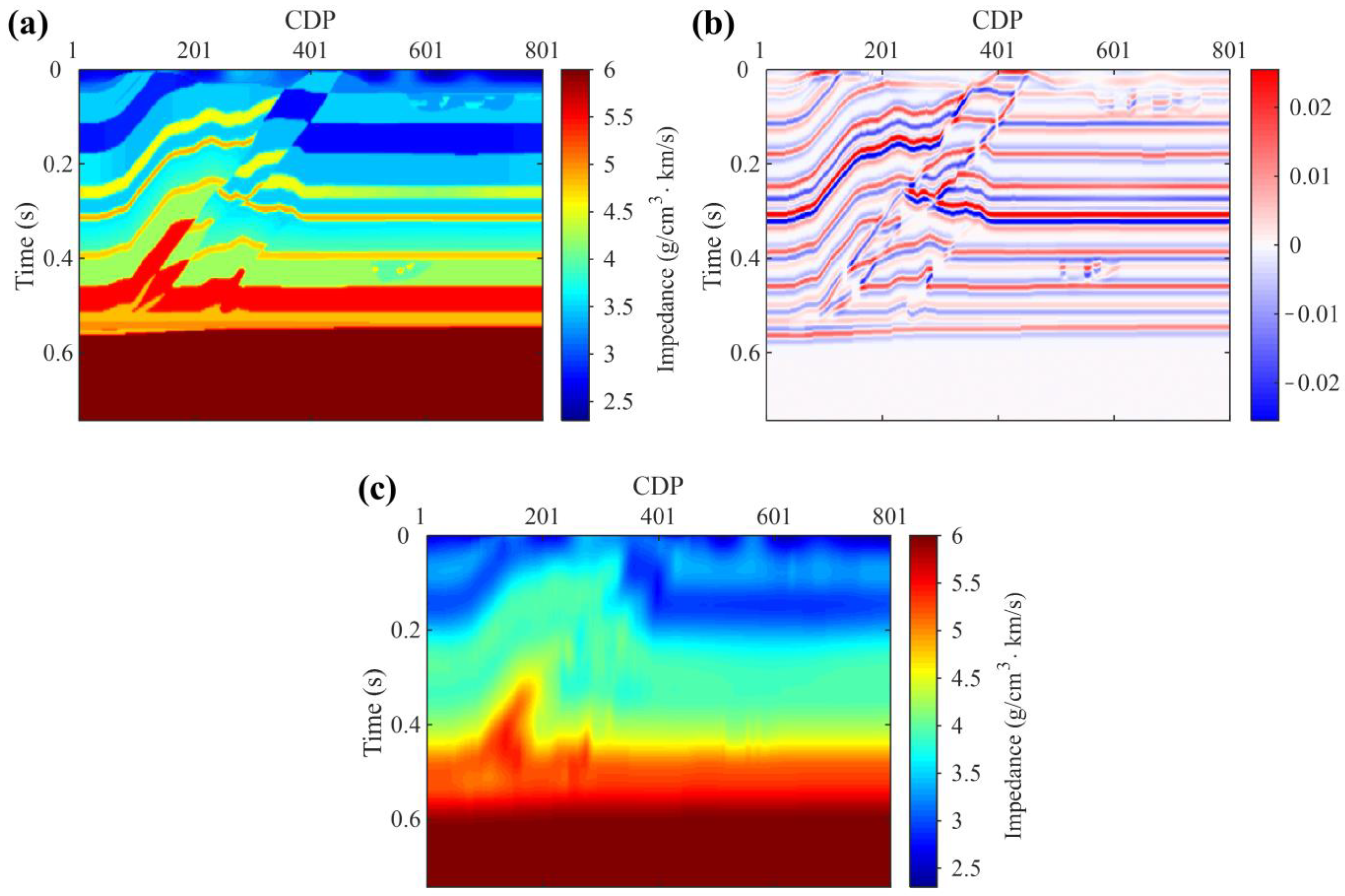
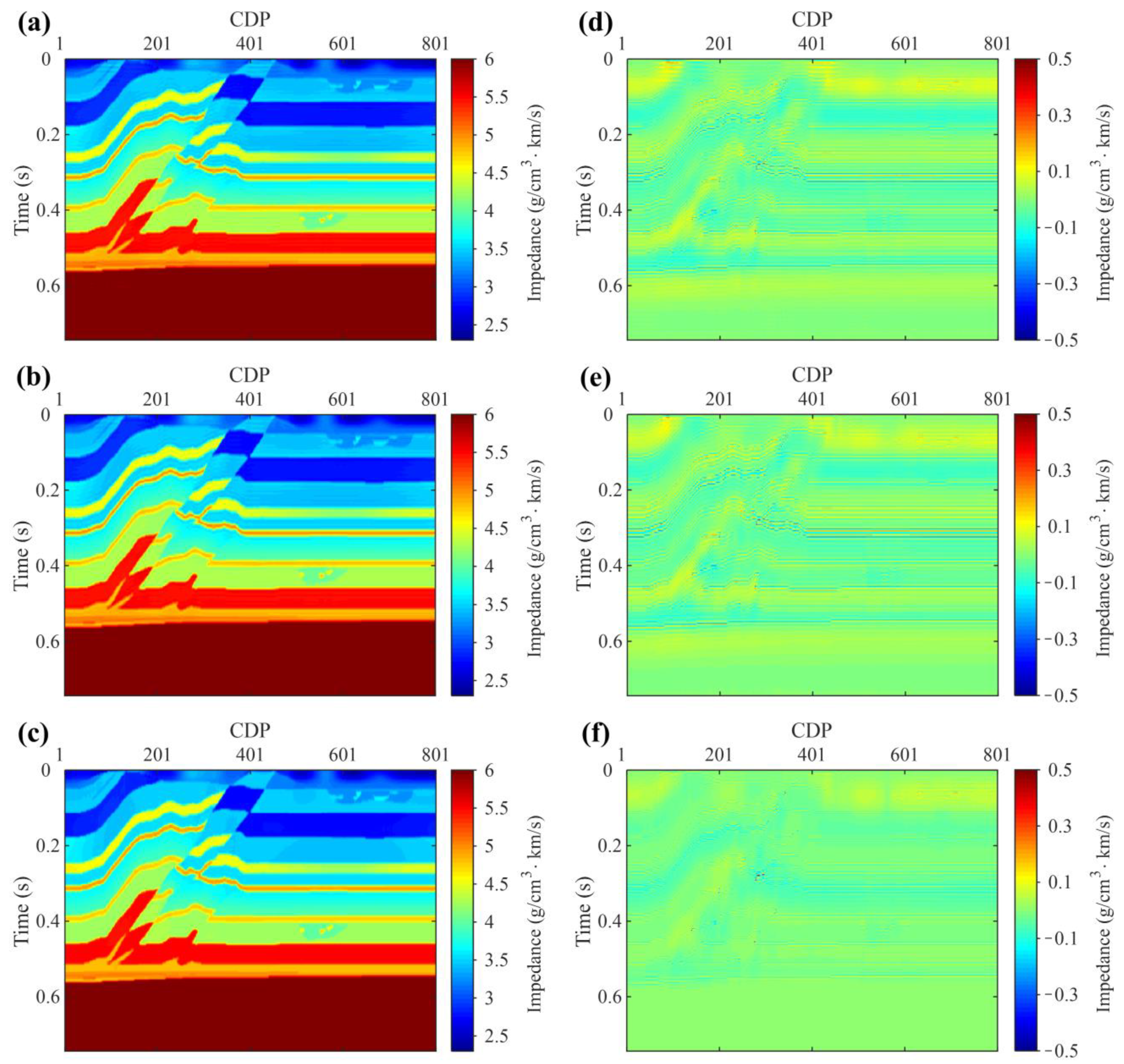
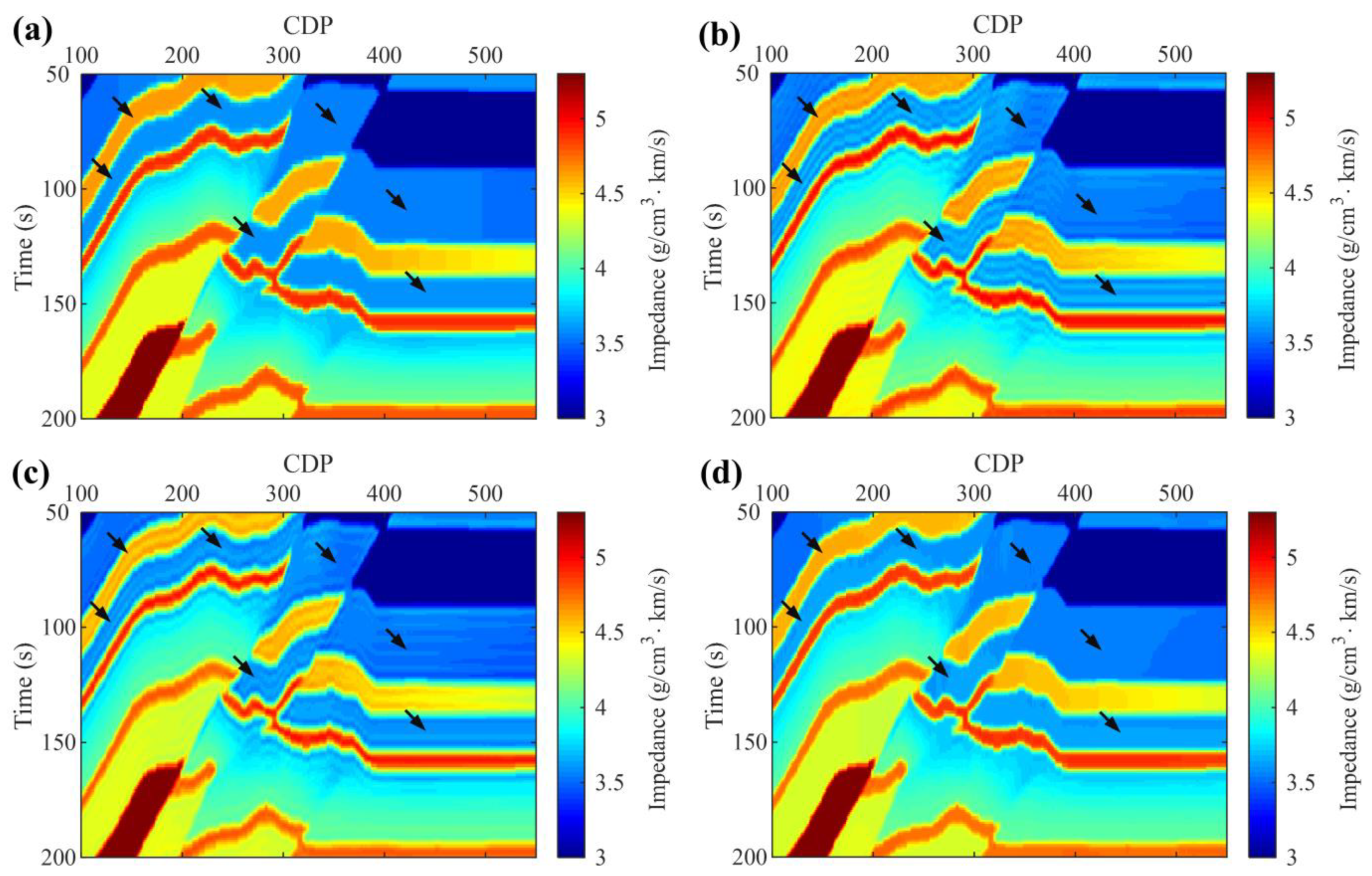
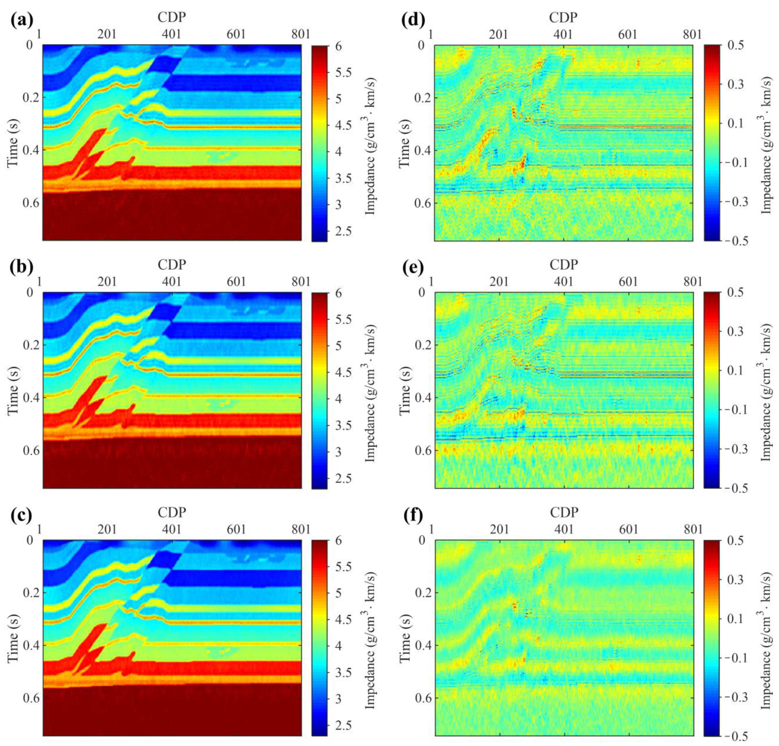
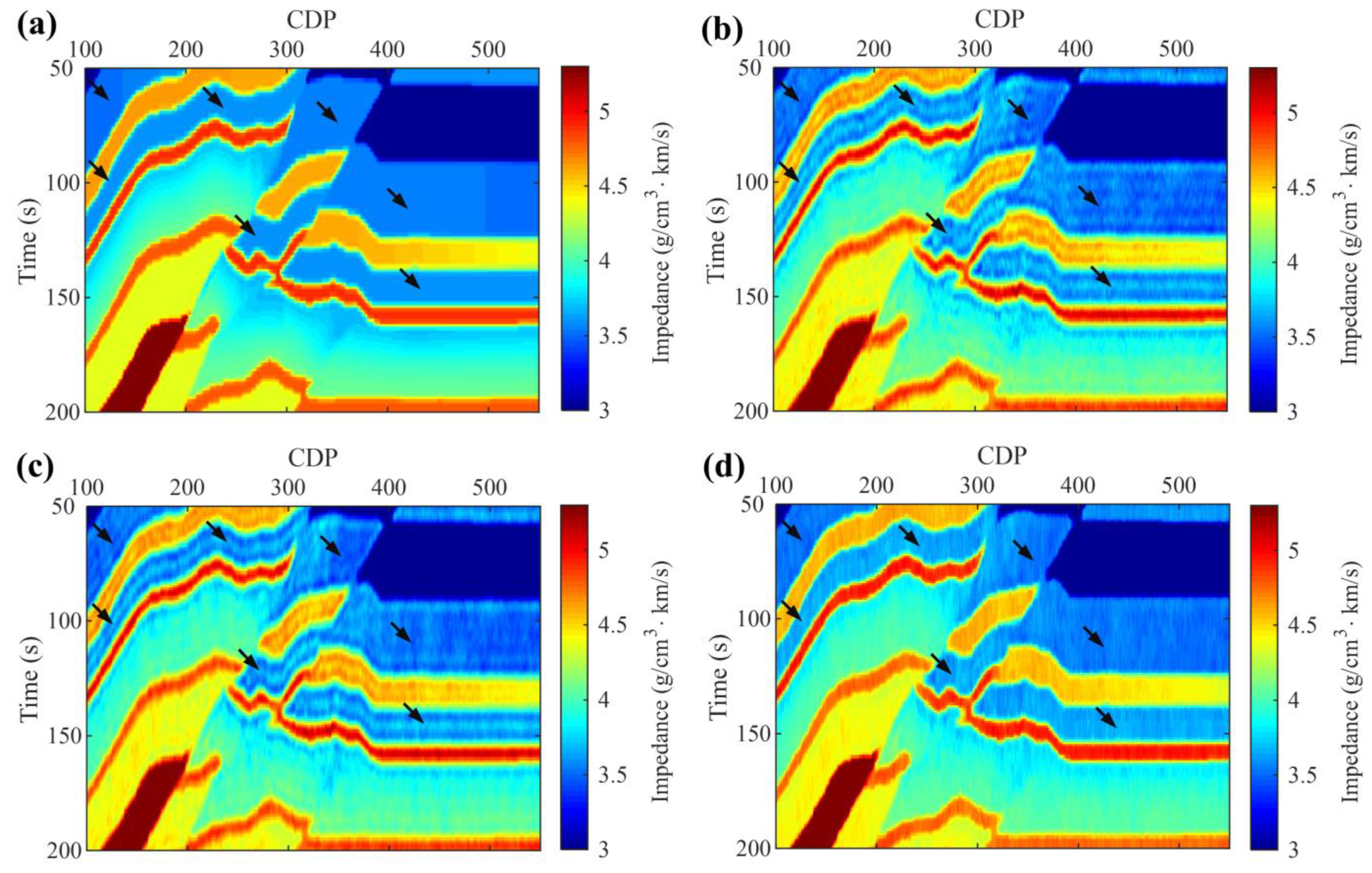
First, we check the effectiveness of the developed methods with the SEG/EAGE overthrust impedance model (Figure 2a). Figure 2b depicts the noise-free seismic profile synthesized by convolving a 30 Hz Ricker wavelet with the reflection coefficients calculated in Figure 2a. This profile contains 801 traces and 373 sampling points with a sampling interval of 2 ms. The conventional MII, LMII, and constrained LMII methods are used for impedance inversion, and their inversion results are presented in Figure 3a–c, respectively. For the above methods, they are set to the same stopping criterion, i.e., the algorithm stops when the number of iterations is greater than 500 or the tolerance error is less than 10−6. It should be noted that the low-frequency reference model (Figure 2c) utilized in the above three methods is obtained by performing 10 Hz low-pass filtering on Figure 2a. In addition, the measurement ratios of seismic data and reference model are set to 0.45 and 0.1 in the LMII and constrained LMII methods, respectively. As shown in Figure 3a–c, all these methods effectively recover small-scale geological information such as thin layers, lenses, pinch-outs, and channels. Figure 3d–f depicts the difference between the results inverted by the above three methods and the true impedance. As observed from Figure 3d–f, the residuals of the conventional MIII method and the LMII method are basically the same, while the residuals of the constrained LMII method are significantly smaller than the other two methods. This indicates that introducing the EH norm effectively improves inversion accuracy. In other words, the EH norm is more accurate than the conventional Tikhonov regularization in characterizing the subsurface structure. To visually compare the advantages and disadvantages of the three methods, Figure 4 displays the zoomed-in views of the true impedance and the inversion results of Figure 3. Figure 4 demonstrates that the inversion results obtained by the MII and LMII methods are oversmooth, blurring the stratigraphic boundaries and producing additional pseudo-layer interferences (as shown by the arrows). In contrast, the inversion results yielded by the constrained LMII method show stratigraphic boundaries more clearly, while greatly avoiding erroneous pseudo-layer interferences.
In order to quantitatively evaluate the reliability of these inverted results, root mean square error (RMSE) defined by the following equation is used as the evaluation index:
R M S E = 1 M × N i = 1 M j = 1 N ( z ¯ i j y i j ) 2
where y denotes the true impedance, z ¯ denotes the predicted impedance, M and N represent the number of sampling points and the number of seismic traces, respectively. Note that a smaller RMSE means higher reliability of the predicted impedance. The quantitative comparison of the inverted results of Figure 3 is listed in Table 1. As seen in Table 1, the constrained LMII method achieves a smaller RMSE value than the other two methods. This further demonstrates that the constrained LMII method can recover the impedance of subsurface rock more precisely. Moreover, the RMSE values obtained by the MII and LMII methods are basically consistent, but the calculation time of the conventional MII method is obviously longer than that of the LMII method. This provides reliable proof that the LMII method can effectively improve inversion efficiency while maintaining inversion accuracy. It should be pointed out that although the constrained LMII method uses an efficient alternating multiplier iteration algorithm to solve its objective function, it is slightly longer than the LMII method in terms of computational time due to the non-convex optimization involved. Notwithstanding, the constrained LMII method still has an advantage in computational efficiency compared to the conventional MII method.
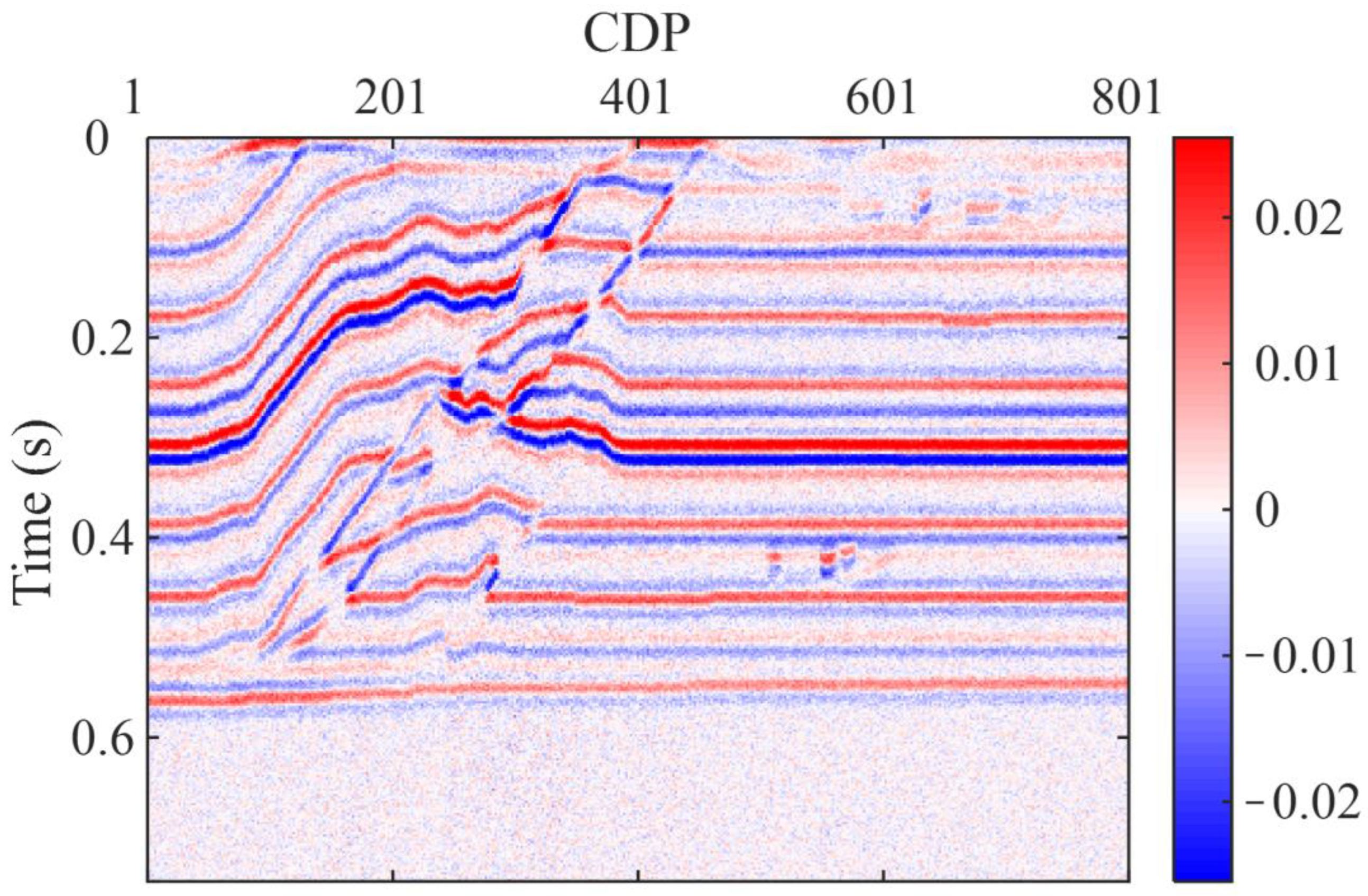
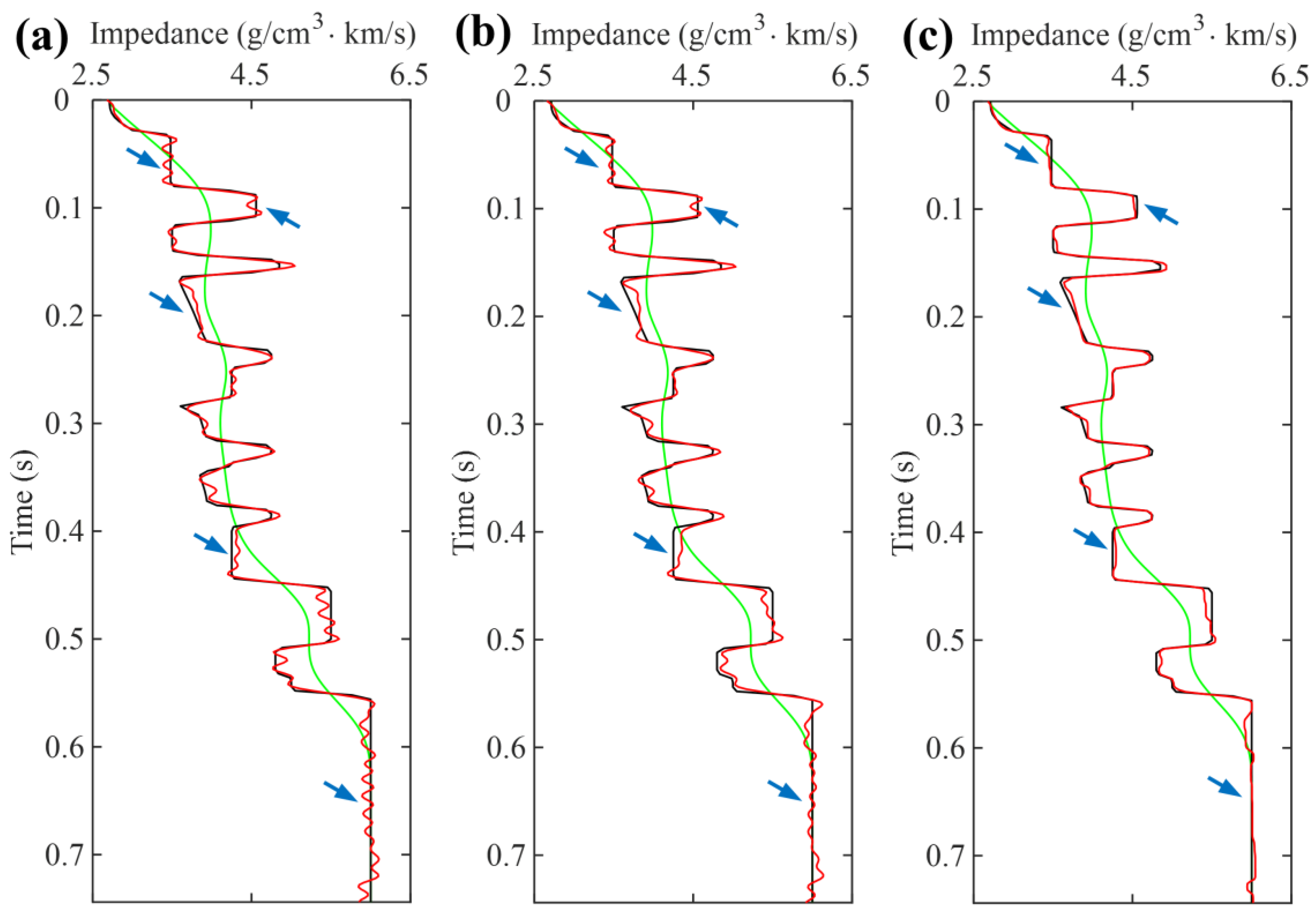
To test the stability of the developed LMII and constrained LMII methods, we add Gaussian noise with a signal-to-noise ratio (SNR) of 3 (whose mean is 0 and standard deviation is one-third of the root mean square of the signal) to Figure 2b and obtain a noisy seismic profile for impedance inversion (Figure 5). In this case, the reference model and the setting of measurement ratios are the same as in the noise-free experiment. Figure 6a–c presents the results inverted by MII, LMII, and constrained LMII methods, respectively. Figure 6d–f presents the residuals between these inversion results and the true impedance, respectively. Note that the maximum number of iterations and tolerance error for the above methods are set to 500 and 10−3. As observed from Figure 6, all inversion methods can recover impedance from noise-contaminated seismic data. Nevertheless, the constrained LMII method is significantly better than the other two methods in terms of accuracy since the constrained LMII method achieves a smaller residual. For better comparison, a zoomed window of the true impedance and the inverted results of Figure 6 are shown in Figure 7. At the same time, Figure 8 compares the impedance curves of the 300th trace of the inversion results shown in Figure 6. It can be seen from Figure 7 and Figure 8 that the impedance interfaces of the MII and LMII methods are blurred, while the pseudo-layer interferences are obvious (as shown by arrows). In contrast, the impedance inverted by the constrained LMII method is much better than the other two methods, where the prediction errors are lower, and the layer interfaces are clear. To quantitatively evaluate the inversion quality, we calculate the RMSE values of the three inversion results and show them in Table 2. Also, the elapsed time of the above three inversion methods is listed in Table 2. From Table 2, it can be found that the inversion accuracy of the LMII method is essentially the same as that of the traditional MII methods, while the elapsed time is reduced by nearly half. This further illustrates the advantage of the LMII method in improving inversion efficiency. Besides, it can also be found from Table 2 that the constrained LMII method has a smaller RMSE value than the other two methods, which again effectively proves that the constrained LMII method is effective in improving the inversion quality. At the same time, this result also validates that the constrained LMII method has better robustness under noise circumstances.

3.2. Field Example

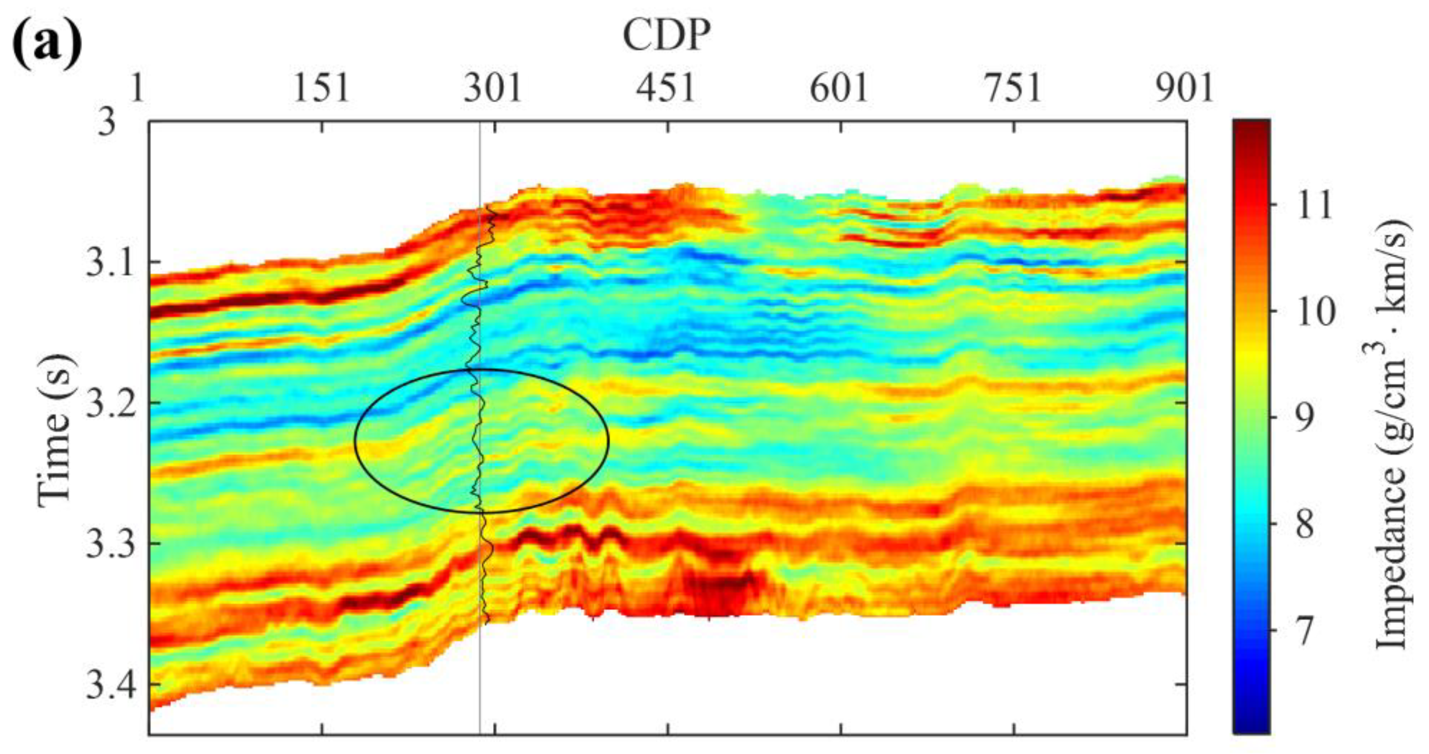
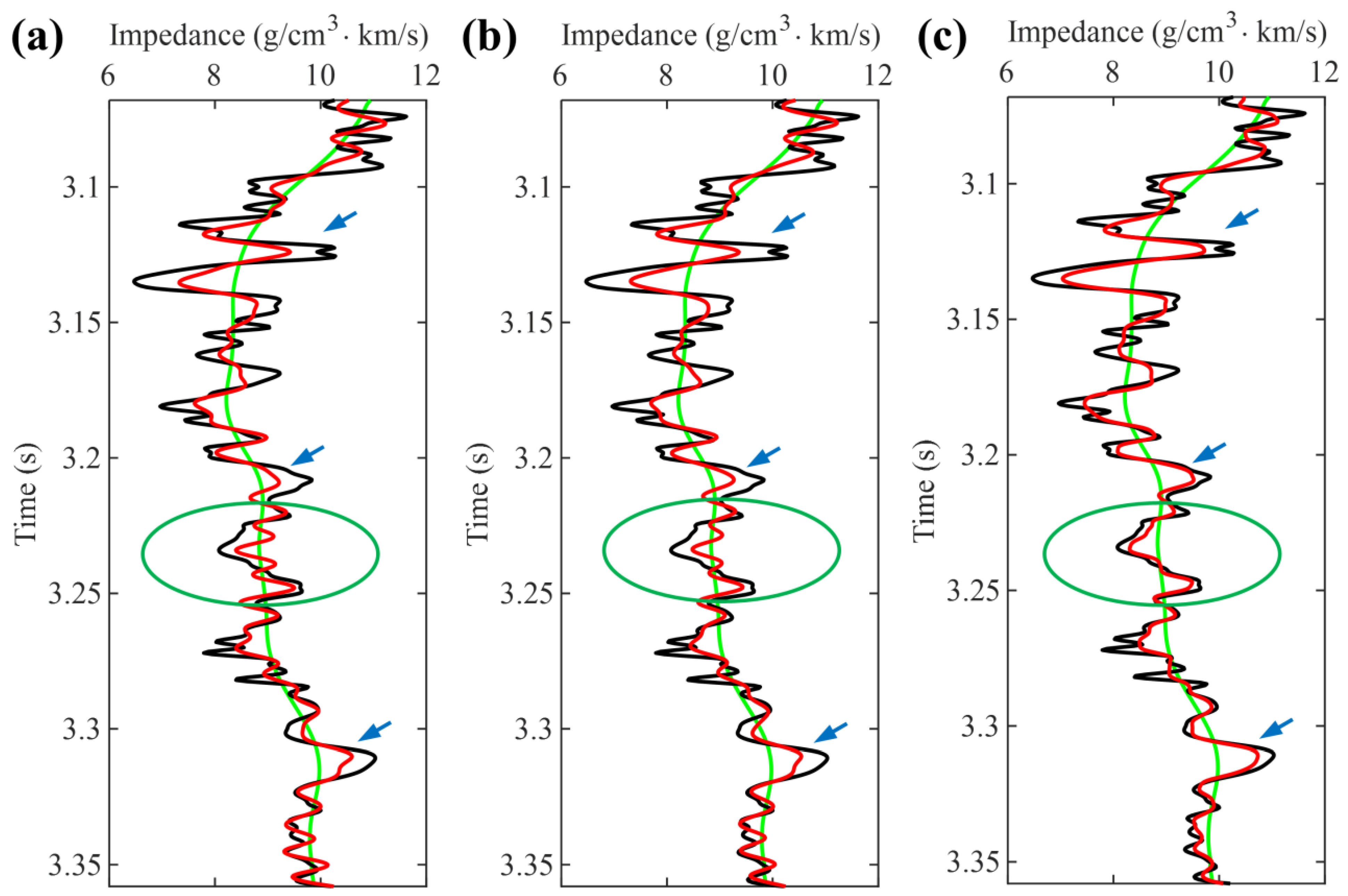
In this subsection, we apply the developed algorithms to the field data to test their practicability for real data inversion. Figure 9a shows 2D field post-stack data, which consists of 901 traces, each containing 300 sampling points with an interval of 1 ms. Therein, a blind well at the 288th trace (shown as the gray line) to judge the reliability of the predicted result. Note that this blind well does not participate in the inversion procedure. Figure 9b displays the low-frequency reference model used for impedance inversion, which is derived by interpolation from the 12–14 Hz high-cut filtered log data within the work area. Figure 10a–c presents the results predicted by the MII, LMII, and constrained LMII methods, respectively. In this case, the maximum number of iterations and the tolerance error of the above methods are set to 500 and 10−5, respectively. In addition, the measurement ratios of the seismic record and reference model are set to 0.25 and 0.1 in the LMII and constrained LMII methods, respectively. It is evident from Figure 10 that the inversion results obtained by all three methods well reflect the lateral extension and lithological variation patterns of the geological bodies. Nevertheless, one notices that the constrained LMII method performs better than the other two methods in identifying the stratigraphic boundaries. Specifically, the results inverted by the constrained LMII method (Figure 10c) have obvious blocky characteristics and show clear geological boundaries, while the results inverted by the other two are over-smooth, blurring the lithological boundary features and leading to difficulties in layer identification. Additionally, the conventional MII method and the LMII method also produce additional pseudo-layer interferences (as shown in the elliptical zone). To better illustrate this point, Figure 11a–c presents the measured well logging curve at the 288th trace and the predicted impedance by the above three inversion methods, respectively. Herein, the green line represents the low-frequency reference curve, the black line represents the logging data, and the red line represents the predicted impedance curve. It is clear from Figure 11 that these inversion results show similar trends to the well log, but the inverted curve by the constrained LMII approach is more consistent with the well log (as shown by the arrows). In addition, as seen in the logging curve, a low-impedance shale layer exists near 3.23 s. After inversion by the conventional MII method and the LMII method, pseudo-layer interferences are generated in their results, which led to the appearance of false sand-shale interbeds. In contrast, the constrained LMII method effectively avoids the pseudo-layer interferences and correctly identifies this stratum. It reveals that the constrained LMII method outperforms the other two methods in terms of inversion reliability, which is consistent with the synthetic examples. In this case, the running times of the MII method, the LMII method, and the constrained LMII method are 298.74, 138.19, and 152.21 s, respectively. Clearly, both LMII and constrained LMII methods have smaller computing costs compared with the MII method, which further demonstrates that it is effective to compress the size of the inverse problem by low-dimensional measurements in sparse space.

4. Discussion

Investigating the sensitivity of the impedance inversion algorithm to the estimation accuracy of the source wavelet has important guiding significance for its subsequent practical application. Herein, we take Figure 2 as an example to study the sensitivity of the proposed methods to the source wavelet. Figure 12 shows the relationship curves between the quantitative evaluation index (RMSE) of inversion results by the proposed algorithms and wavelet estimation accuracy. As shown in Figure 12, the smallest RMSE value is obtained when the exact wavelet (i.e., frequency of 30 Hz) is used as the input of the LMII and constrained LMII algorithms. This means that both LMII and constrained LMII algorithms achieve the highest inversion accuracy at this time. With the decrease in the wavelet estimation accuracy, the RMSE value of inversion results yielded by the LMII and constrained LMII methods gradually increases. This result demonstrates that the performance of the LMII and constrained LMII methods has a strong dependence on the estimation accuracy of the source wavelet. Therefore, in order to achieve a satisfactory inversion result, the exact source wavelet must be extracted before applying the LMII and constrained LMII methods for impedance inversion.
Although the developed method effectively improves the computational accuracy and efficiency of the multi-trace impedance inversion, it is not flawless and is prone to suffering from lateral smearing when dealing with highly dipping structures. The reason is that the lateral constraint term constructed by the second-order difference operator only forces lateral smoothing and ignores the morphology of underground structures [26]. Recently, structure-oriented multi-trace impedance inversion methods [26,30,31] have effectively solved the lateral smearing problem and can be better adapted to inversion work in regions with large dips. However, similar to the traditional multi-trace impedance method, these methods also suffer from insufficient inversion efficiency and accuracy. Fortunately, the inversion framework presented in this paper has excellent expansibility. Therefore, combining the proposed inversion framework with structure-oriented multi-trace inversion methods to develop a series of novel impedance inversion algorithms that can adapt to highly dipping structures with high computational efficiency and accuracy will be a future research direction.

5. Conclusions

To address the issues existing in the conventional MII method with low efficiency and accuracy, a low-dimensional multi-trace inversion method with elastic half norm constraints is proposed. First, we develop an LMII inversion framework that efficiently reduces the scale of the MII inversion problem and thus achieves efficient inversion. Concretely, this framework converts the seismic data and reference impedance into the sparse space by an orthogonal transformation and constructs the objective function with a smaller size for multi-trace inversion using the low-dimensional measurements in the sparse domain. Subsequently, on the basis of the developed LMII framework, we introduce the EH norm as a vertical constraint on the model parameters and propose a novel constrained LMII model for inverting the subsurface impedance. Since this inversion procedure considers both the smoothness and blockiness of the subsurface strata, it can significantly improve the inversion precision compared with the traditional MII method, which considers smoothness only. Finally, based on the variable splitting technique, we derive an alternating multiplier iteration algorithm to efficiently solve the constrained LMII problem. Two experiments are conducted to investigate the performance of the developed algorithms. The results indicate that the LMII framework can effectively improve the multi-trace inversion efficiency while keeping the inversion accuracy constant. Meanwhile, it is also shown that the constrained LMII model can evidently promote the quality of impedance inversion while inheriting the efficiency of the LMII framework. In addition, it should be pointed out that the proposed methods have good scalability and can be extended to gravity inversion, magnetic inversion, and other fields to provide new insights for solving more geophysical problems.

Author Contributions

Conceptualization, N.L. and F.Z.; methodology, N.L., F.Z. and K.X.; software, N.L., F.Z. and K.X.; validation, N.L., F.Z. and H.Z.; formal analysis, N.L., F.Z. and Y.L.; investigation, N.L., F.Z. and Y.L.; resources, N.L., H.Z. and K.X.; data curation, N.L., H.Z. and Y.L.; writing—original draft preparation, N.L.; writing—review and editing, N.L., F.Z., H.Z. and Y.L.; funding acquisition, F.Z. All authors have read and agreed to the published version of the manuscript.

Funding

This research is supported by the Laoshan National Laboratory of Science and Technology Foundation (No. LSKJ202203400) and the National Natural Science Foundation of China (No. 42030103).

Data Availability Statement

Not applicable.

Acknowledgments

We are grateful to the editor and all the reviewers for their constructive comments on this paper. We would also like to thank the Laoshan National Laboratory of Science and Technology Foundation and the National Natural Science Foundation of China for their financial support during this research.

Conflicts of Interest

The authors declare no conflict of interest.

References

  1. Harrison, C.B. Feasibility of Rock Characterization for Mineral Exploration Using Seismic Data. Ph.D. Thesis, Curtin University, Perth, Australia, 2009. [Google Scholar]
  2. Kieu, D.T.; Kepic, A. Seismic-impedance inversion with fuzzy clustering constraints: An example from the Carlin Gold district, Nevada, USA. Geophys. Prospect. 2020, 68, 103–128. [Google Scholar] [CrossRef] [Green Version]
  3. Donoso, G.A.; Bautista, C.; Malehmir, A.; Araujo, V. Characterizing volcanogenic massive sulphides using acoustic impedance inversion, Neves-Corvo, southern Portugal. In NSG2022 4th Conference on Geophysics for Mineral Exploration and Mining; European Association of Geoscientists and Engineers: Belgrade, Serbia, 2022; pp. 1–5. [Google Scholar]
  4. Russell, B.; Hampson, D. Comparison of poststack seismic inversion methods. In SEG Technical Program Expanded Abstracts 1991; Society of Exploration Geophysicists: Houston, TX, USA, 1991; pp. 876–878. [Google Scholar]
  5. Dai, R.; Yin, C.; Zaman, N.; Zhang, F. Seismic inversion with adaptive edge-preserving smoothing preconditioning on impedance model. Geophysics 2019, 84, R25–R33. [Google Scholar] [CrossRef]
  6. Tikhonov, A. On the solution of ill-posed problems and the method of regularization. Dokl. Akad. Nauk. SSSR 1963, 151, 501–504. [Google Scholar]
  7. VanDecar, J.C.; Snieder, R. Obtaining smooth solutions to large, linear, inverse problems. Geophysics 1994, 59, 818–829. [Google Scholar] [CrossRef]
  8. Sacchi, M.D. Reweighting strategies in seismic deconvolution. Geophys. J. Int. 1997, 129, 651–656. [Google Scholar] [CrossRef] [Green Version]
  9. Gholami, A.; Siahkoohi, H.R. Regularization of linear and nonlinear geophysical ill-posed problems with joint sparsity constraints. Geophys. J. Int. 2010, 180, 871–882. [Google Scholar] [CrossRef] [Green Version]
  10. Aghamiry, H.S.; Gholami, A.; Operto, S. Compound regularization of full waveform inversion for imaging piecewise media. IEEE Trans. Geosci. Romote Sens. 2020, 58, 1192–1204. [Google Scholar] [CrossRef] [Green Version]
  11. Zhang, F.; Dai, R.; Liu, H. Seismic inversion based on L1-norm misfit function and total variation regularization. J. Appl. Geophys 2014, 109, 111–118. [Google Scholar] [CrossRef]
  12. Gholami, A. Nonlinear multichannel impedance inversion by total-variation regularization. Geophysics 2015, 80, R217–R224. [Google Scholar] [CrossRef]
  13. Li, C.H.; Zhang, F.C. Amplitude-versus-angle inversion based on the L1-norm-based likelihood function and the total variation regularization constraint. Geophysics 2017, 82, R173–R182. [Google Scholar] [CrossRef]
  14. Guo, S.; Wang, H. Seismic absolute acoustic impedance inversion with L1 norm reflectivity constraint and combined first- and second-order total variation regularizations. J. Geophys. Eng. 2019, 16, 773–788. [Google Scholar] [CrossRef]
  15. Dai, R.; Yang, J. An alternative method based on region fusion to solve L0-norm constrained sparse seismic inversion. Explor. Geophys. 2021, 52, 624–632. [Google Scholar] [CrossRef]
  16. Zhang, R.; Castagna, J. Seismic sparse-layer reflectivity inversion using basis pursuit decomposition. Geophysics 2011, 76, R147–R158. [Google Scholar] [CrossRef] [Green Version]
  17. Zhang, R.; Sen, M.K.; Srinivasan, S. A prestack basis pursuit seismic inversion. Geophysics 2013, 78, R1–R11. [Google Scholar] [CrossRef]
  18. Wang, L.; Zhou, H.; Liu, W.; Yu, B.; He, H.; Chen, H.; Wang, N. Data-driven multichannel poststack seismic impedance inversion via patch-ordering regularization. Geophysics 2021, 86, R197–R210. [Google Scholar] [CrossRef]
  19. Wang, G.; Chen, S. Pre-stack seismic inversion with L1-2-norm regularization via a proximal dc algorithm and adaptive strategy. Surv. Geophys. 2022, 43, 1817–1843. [Google Scholar] [CrossRef]
  20. Ma, M.; Zhang, R.; Yuan, S.Y. Multichannel impedance inversion for nonstationary seismic data based on the modified alternating direction method of multipliers. Geophysics 2019, 84, A1–A6. [Google Scholar] [CrossRef]
  21. Zhang, F.C.; Liu, J.; Yin, X.Y.; Yang, P.J. Modified Cauchy-constrained seismic blind deconvolution. Oil Geophys. Prospect. 2008, 43, 391–396. [Google Scholar]
  22. Dai, R.; Zhang, F.; Liu, H. Seismic inversion based on proximal objective function optimization algorithm. Geophysics 2016, 81, R237–R246. [Google Scholar] [CrossRef]
  23. Sun, J.; Li, Y. Adaptive Lp inversion for simultaneous recovery of both blocky and smooth features in a geophysical model. Geophys. J. Int. 2014, 197, 882–899. [Google Scholar] [CrossRef] [Green Version]
  24. Hamid, H.; Pidlisecky, A. Multitrace impedance inversion with lateral constraints. Geophysics 2015, 80, M101–M111. [Google Scholar] [CrossRef]
  25. Yuan, S.Y.; Wang, S.X.; Luo, C.M.; He, Y.X. Simultaneous multitrace impedance inversion with transform-domain sparsity promotion. Geophysics 2015, 80, R71–R80. [Google Scholar] [CrossRef]
  26. Hamid, H.; Pidlisecky, A. Structurally constrained impedance inversion. Interpretation 2016, 4, T577–T589. [Google Scholar] [CrossRef]
  27. Dai, R.; Zhang, F.; Yin, C.; Hu, Y. Multi trace post stack seismic data sparse inversion with nuclear norm constraint. Acta Geophys. 2021, 69, 53–64. [Google Scholar] [CrossRef]
  28. Yang, Y.; Xia, X.; Yin, X.; Li, K.; Wang, J.; Liu, H. Data-driven fast prestack structurally constrained inversion. Geophysics 2022, 87, N31–N43. [Google Scholar] [CrossRef]
  29. Karimi, P. Structure constrained relative acoustic impedance using stratigraphic coordinates. Geophysics 2015, 80, A63–A67. [Google Scholar] [CrossRef]
  30. Yin, X.Y.; Yang, Y.M.; Li, K.; Man, J.; Li, H.; Feng, Y. Multitrace inversion driven by cross-correlation of seismic data. Chin. J. Geophys. 2020, 63, 3827–3837. [Google Scholar]
  31. Zhang, Y.; Wu, W.; Zhang, M.; Liang, M.; Feng, B. Multitrace Impedance Inversion Based on Structure-Oriented Regularization. IEEE Geosci. Remote Sens. Lett. 2021, 19, 1–5. [Google Scholar] [CrossRef]
  32. Donoho, D.L. Compressed sensing. IEEE Trans. Inf. Theory 2006, 52, 1289–1306. [Google Scholar] [CrossRef]
  33. Baraniuk, R.G. Compressive sensing. IEEE Signal Process. Mag. 2007, 24, 118–121. [Google Scholar] [CrossRef]
  34. Lan, N.Y.; Zhang, F.C.; Li, C.H. Robust high-dimensional seismic data interpolation based on elastic half norm regularization and tensor dictionary learning. Geophysics 2021, 86, V431–V444. [Google Scholar] [CrossRef]
  35. Lions, P.L.; Mercier, B. Splitting algorithms for the sum of two nonlinear operators. SIAM J. Numer. Anal. 1979, 16, 964–979. [Google Scholar] [CrossRef]
  36. Lan, N.Y.; Zhang, F.C. Seismic data recovery using deep targeted denoising priors in an alternating optimization framework. Geophysics 2022, 87, V279–V291. [Google Scholar] [CrossRef]
  37. Berteussen, K.; Ursin, B. Approximate computation of the acoustic impedance from seismic data. Geophysics 1983, 48, 1351–1358. [Google Scholar] [CrossRef]
  38. Barrett, R.; Berry, M.; Chan, T.F.; Demmel, J.; Donato, J.M.; Dongarra, J.; Eijkhout, V.; Pozo, R.; Romine, C.; Van der Vorst, H. Templates for the Solution of Linear Systems: Building Blocks for Iterative Methods; Society for Industrial and Applied Mathematics: Philadelphia, PA, USA, 1994; pp. 64–68. [Google Scholar]
  39. Candes, E.; Romberg, J.; Tao, T. Robust uncertainty principles: Exact signal reconstruction from highly incomplete frequency information. IEEE Trans. Inf. Theory 2006, 52, 489–509. [Google Scholar] [CrossRef] [Green Version]
  40. Huang, H.; Misra, S.; Tang, W.; Barani, H.; Al-Azzawi, H. Applications of compressed sensing in communications networks. arXiv 2014, arXiv:1305.3002. [Google Scholar]
  41. Xu, Z.B.; Chang, X.Y.; Xu, F.; Zhang, H. L1/2 regularization: A thresholding representation theory and a fast solver. IEEE Trans. Neural Netw. Learn. Syst. 2012, 23, 1013–1027. [Google Scholar]
  42. Sorensen, H.V.; Jones, D.L.; Burrus, C.S.; Heideman, M.T. On computing the discrete Hartley transform. IEEE Trans. Acoust. Speech Signal Process. 1985, 33, 1231–1238. [Google Scholar] [CrossRef]
Figure 1. Verification of the validity of DHT domain conversion: (a) Impedance model; (b) Low-frequency reference model; (c) Synthetic seismic data; (d,e) DHT coefficients of low-frequency reference model and synthetic seismic data, respectively. The DHT coefficients for both the low-frequency reference model and the synthetic data are distributed at the low-frequency end. This indicates that DHT can concentrate signal energy in the low-frequency part of the spectrum.
Minerals 13 00972 g001
Figure 2. Synthetic example: (a) Theoretical overthrust impedance model; (b) Synthetic noise-free seismic profile; (c) Low-frequency reference model.
Minerals 13 00972 g002
Figure 3. Comparison of the inversion results obtained by different methods in the noise-free case: (a) Inversion results by MII; (b) Inversion results by LMII; (c) Inversion results by constrained LMII; (d) Difference between (a) and the true impedance; (e) Difference between (b) and the true impedance; (f) Difference between (c) and the true impedance.
Minerals 13 00972 g003
Figure 4. Zoomed-in view of the inversion results shown in Figure 3: (a) Zoomed-in view of the true model; (bd) Zoomed-in views of Figure 3a–c, respectively.
Minerals 13 00972 g004
Figure 5. Seismic profile with SNR = 3.
Minerals 13 00972 g005
Figure 6. Comparison of inversion results by different methods in the noisy case: (ac) present inversion results by MII, LMII, and constrained LMII, respectively; (df) present their residuals with the true impedance, respectively.
Minerals 13 00972 g006
Figure 7. Zoomed-in comparison of the inversion results of Figure 6: (a) Zoomed-in view of Figure 2a; (bd) Zoomed-in views of Figure 6a–c, respectively.
Minerals 13 00972 g007
Figure 8. Comparison of the 300th trace from the inversion results of Figure 6: (ac) present inversion results by MII, LMII, and constrained LMII, respectively. The green, black, and red lines represent the low-frequency reference model, true model, and inverted impedance, respectively.
Minerals 13 00972 g008
Figure 9. Field example: (a) 2D post-stack seismic profile; (b) Low-frequency reference model.
Minerals 13 00972 g009
Figure 10. Comparison of inversion results by different methods for the field data: (ac) present inversion results by MII, LMII, and constrained LMII, respectively. The grey and black lines represent the location of the blind well as well as the well log, respectively.
Minerals 13 00972 g010aMinerals 13 00972 g010b
Figure 11. Comparison of the 288th trace from the inversion results of Figure 10: (ac) present inversion results by MII, LMII, and constrained LMII, respectively. The green, black, and red lines represent the low-frequency reference model, well log, and inverted impedance curve, respectively. The well log shows a low-impedance shale layer at the green circle. The MII and LMII methods produce pseudo-layer interferences, resulting in false sand-shale interbeds at this location. The constrained LMII method effectively avoids the pseudo-layer interferences and correctly identifies this formation.
Minerals 13 00972 g011
Figure 12. Relationship curves between the quantitative evaluation index (RMSE) of inversion results and wavelet estimation accuracy.
Minerals 13 00972 g012
Table 1. Quantitative evaluation index and running time of the inversion results of Figure 3.
MethodRMSE (×10−3)Time (s)
MII46.10261.89
LMII46.11135.13
Constrained LMII29.06161.17
Table 2. Quantitative evaluation index and running time of the inversion results of Figure 6.
MethodRMSE (×10−3)Time (s)
MII79.93269.31
LMII79.94138.28
Constrained LMII57.92165.80
Disclaimer/Publisher’s Note: The statements, opinions and data contained in all publications are solely those of the individual author(s) and contributor(s) and not of MDPI and/or the editor(s). MDPI and/or the editor(s) disclaim responsibility for any injury to people or property resulting from any ideas, methods, instructions or products referred to in the content.