Article

Estimation of Carbon Content in High-Ash Coal Using Mid-Infrared Fourier-Transform Infrared Spectroscopy

1
Photogeology and Image Processing Laboratory, Department of Applied Geology, Indian Institute of Technology (Indian School of Mines), Dhanbad 826004, India
2
Coal Geology and Organic Petrology Laboratory, Department of Applied Geology, Indian Institute of Technology (Indian School of Mines), Dhanbad 826004, India
*
Author to whom correspondence should be addressed.
Minerals 2023, 13(7), 938; https://doi.org/10.3390/min13070938
Submission received: 12 April 2023 / Revised: 11 July 2023 / Accepted: 11 July 2023 / Published: 13 July 2023
(This article belongs to the Special Issue Coal: Chemical, Geochemical and Petrographical Aspects)

Abstract

:
The carbon content of different types of coal determines its utility in industries and thermal power generation. The most popular and widely used is the conventional method (ultimate analysis) to determine coal’s carbon content (C, wt.%), along with H, N, and S. In the present study, the authors attempted to analyze the carbon content (C in %) in coals via data from Fourier-transform infrared (FTIR) spectroscopy, which can be a promising alternative. As a reference, the carbon content in the coal samples, referred to as CCHNS (in wt.%), was determined from the ultimate analysis. The mid-infrared FTIR spectroscopic data were used to investigate the response of functional groups associated with carbon or its compounds, which were used to model and estimate the carbon content in coal samples (referred to as CFTIR, in wt.%). FTIR spectral signatures were utilized in specific zones (between wavenumbers 4000 and 400 cm−1) from a total of 18 coal samples from the Johilla coalfield, Umaria district, Madhya Pradesh, India. These 18 coal samples were used to produce 126 Coal+KBr pellets (at seven known dilution factors for each coal sample), and the spectral response (absorbance) from each pellet was recorded. For model development and validation, the training set and test set were formed using a 17:1 split (K-fold cross validation). The carbon content in the coal samples was modeled using the training set data by applying the piecewise linear regression method employing quasi-Newton (QN) with a breakpoint and least squares loss function. The model was validated using an independent test set. A pairwise comparison of estimates of carbon in the laboratory from the CHNS analyzer (CCHNS) and modeled carbon from FTIR data (CFTIR) exhibited a good correlation, relatively low error, and bias (coefficient of determination (R2) up to 0.93, RMSE of 23.71%, and MBE of −0.52%). Further, the significance tests for the mean and variance using the two-tailed t-test and F-test showed that no significant difference occurred between the pair of observed CCHNS and the model’s estimated CFTIR. For high-ash coals from the Johilla coalfield, the model presented here using mid-infrared FTIR spectroscopy data performs well. Thus, FTIR can potentially serve as an important method for quickly determining the carbon content of high-ash coals from various basins and can potentially be extended to soil and shale samples.

1. Introduction

Coal is an inhomogeneous, naturally occurring, non-renewable energy source and combustible organic rock that contains carbon (C), hydrogen (H), oxygen (O), nitrogen (N), sulfur (S), and various other minor and trace elements. Carbon is a key indicator of coal quality as it constitutes most of the organic matter in coal and is utilized to promptly estimate the coal calorific value [1].
Since the first industrial revolution in the 1800s, coal has been one of the earliest fossil fuels used by humans. The carbon content of coal (organic and inorganic) determines the suitability of its use in different industrial applications. It has been the main source of energy generation because of its abundance and cost. It is used for power and electricity generation and many other industrial uses, like as an essential additive in iron and steel, brickmaking, and the cement industry. Activated carbon, used in filters for water and air purification systems; carbon fiber, used in the construction of automobiles and aircraft; and silicon metal for lubricants are a few products made using coal and coal by-products. Coal accounts for nearly 30% of all global fossil fuel consumption [2].
In India, coal is the sole natural resource and fossil fuel that is readily available throughout the country. Indian coal is mostly found in the Lower Gondwana and Tertiary basins in the central and eastern parts of the country, predominantly with high ash content and low calorific values. Coal remains indispensable worldwide due to the expanding population causing increased demand for electricity and power, especially in emerging nations that lack access to modern, clean energy [3].
The carbon and sulfur content in coal impact the combustion attributes of the coal, pollutant emissions, and also influence coal pricing [4]. The precise determination of the carbon content in coal plays a crucial role in establishing the chemical characterization of fuel commodities. It is essential to substantially improve combustion efficiency and the efficient utilization of equipment, reduce environmental impact, and make informed judgments regarding the appropriateness of coal [4,5]. It also helps to obtain optimal boiler control in the operation of coal-fired thermal power plants. Therefore, it is imperative to create a quick and accurate method for quantifying carbon in coal.
During the combustion process, the generation of carbon dioxide (CO2) poses a significant threat to human health and the global environment [6]. Countries such as China, India, Japan, Russia, the USA, and Australia, which have established coal power industries, consistently report elevated levels of CO2 pollution each year [7]. Coal combustion accounts for about 40% of the world’s CO2 emissions, enhancing the greenhouse effect, and is considered one of the major factors causing climate change [8]. The CO2 along with particulate matter (PM 2.5) affect the air quality. It can adversely affect human health, leading to lung and cardiovascular diseases like asthma and a poor life expectancy [9,10].
In recent years, there has been a significant rise in the use of instrumental analytical techniques to analyze coal and coal products. These methods have become widely accepted as standardized test methods for the analysis of coal by national and international organizations. The ultimate analyzer commonly measures the weight percentage of C, H, N, S, and O (by difference) in a coal sample. The instantaneous examination of coal’s elemental composition is a major requirement in industrial operations. Different firms and laboratories worldwide have employed several test methods for rapidly estimating the carbon content of coal, but these methods have not been established as standardized test methods. Many research works focused on the ultimate analysis and proximate analysis of coal, targeting the carbon content in coal. The use of non-linear correlations has been suggested for calculating the elemental composition of coal [11]. These correlations were developed based on a large and diverse dataset, which included coals of four different ranks and had a wide range of proximate and ultimate analyses. Correlations were also developed using maximum likelihood estimation (MLE), efficiently predicting the elemental compositions for ultimate analysis [12]. Some of the major estimation methods developed by researchers are as follows: X-ray fluorescence spectrometry (XRF) [13,14]; optical emission spectrometry with inductively coupled plasma (ICP-OES) [15,16]; mass spectrometry with inductively coupled plasma (ICP-MS) [17]; laser-induced breakdown spectroscopy (LIBS) [18,19,20,21,22,23]; thermogravimetric Fourier-transform infrared spectroscopy (TG-FTIR) [24], and Fourier-transform infrared spectroscopy (FTIR) [25,26,27]. All of these methods have advantages and constraints, which were preferred for analyses based on requirements and equipment availability.
In the current study, the authors attempted to build a model using the spectral signatures of coal samples that were captured using FTIR spectroscopy in the mid-infrared range (4000 to 400 cm−1). With the help of FTIR data, a prediction model was developed for estimating the carbon content in high-ash Indian coals using the quasi-Newton (QN) method. This FTIR data-based approach is tested for accuracy compared to the traditional ultimate analysis method using the CHNSO analyzer (Make: Elementar, Model: vario MACRO cube, Manufacturer: Elementar Analysensysteme GmbH, Langenselbold, Germany). This technique relies on the concept that carbon compounds absorb specific wavelengths of infrared radiation, thereby enabling the identification and measurement of carbon in coal.
This research article is organized as follows: Section 1 describes the study’s objectives and motivation and presents the previously established methods. Section 2 explains the study area and methodology of this study. Model establishment using training and testing data and the comparison between similar methods of carbon content estimation are discussed in Section 3. The study’s conclusion, including the recommendations for future work, is given in Section 4. A detailed workflow of this study is visualized in Figure 1.

2. Materials and Methods

2.1. Geology of the Study Area

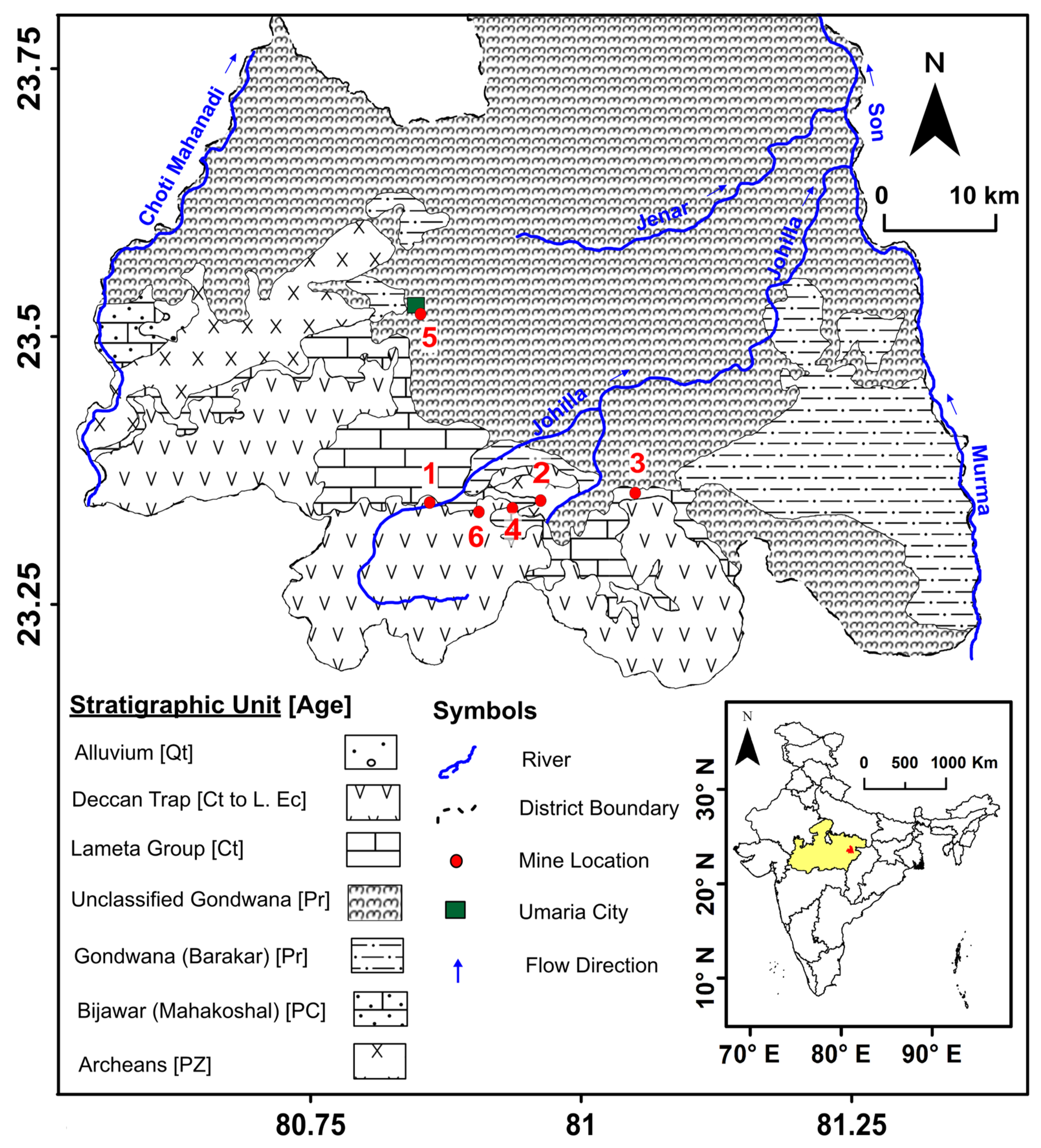
The Johilla coalfield is located in the Umaria district of Madhya Pradesh, India. It is a part of the Son-Narmada Basin and is known for its rich coal deposits [28]. The Johilla coalfield is an important source of coal for industries in the region. The coal-bearing strata in the Johilla coalfield are of the Lower Gondwana age and structurally gently folded and faulted [29,30]. The coal samples from Johilla Coalfield are humic (banded) in nature, corresponding to the sub-bituminous coal rank. The grade of Johilla coals varies from G6 to G7. For this study, 18 coal samples were collected from the Johilla bottom seam, Barakar Formation, following the standard method (ASTM D-2234) [31] from the opencast (OCP) and underground (UG) projects, namely, Kanchan OCP, Kudri UG, Pali UG, Pinoura UG, Umaria UG, and Vindhya UG. A location map of the coal sampling sites is shown in Figure 2. The Barakar Formation comprises sandstones, shales, and coal seams. The collected samples were crushed and sieved to ~212 μm size for FTIR and traditional ultimate analyses, as per guidelines of ASTM D-4749 [32].

2.2. Ultimate Analysis

The ultimate analysis is a traditional method for the determination (in weight percentage) of the elemental composition of coal, mainly the carbon (C), hydrogen (H), nitrogen (N), sulfur (S), and oxygen (O) by difference. ASTM (American Society for Testing and Materials) D5373-08 is the standard method used to determine the total carbon, which includes carbon in the volatile matter. This method can be performed on either an ultimate CHNS or carbon–sulfur analyzer. In the present work, crushed coal samples (~212 µm) were utilized to determine the elemental composition of the coal. For that, 10 mg of samples, sealed inside a tin boat (foil), were placed on an automated sample holder of the CHNS analyzer. The ultimate analysis was conducted at the Department of Applied Geology, Indian Institute of Technology (Indian School of Mines), Dhanbad, Jharkhand, India, in the Vario Macro Cube of Elementar, following the guidelines mentioned in ASTM D-4239 and D-5373 [33,34]. It is a piece of benchtop laboratory equipment calibrated for determining CHNS in coal samples with the highest precision and accuracy. The samples were heated at approximately 1150 °C and 850 °C in combustion and reduction tubes, respectively, in the presence of helium gas purging at a rate of approximately 600 mL/min continuously at 1200–1300 mbar pressure and oxygen (O2) dosing of 50 mL/min for 5 min. Using adsorption and desorption, the equipment carries out the determination of nitrogen (N), carbon (C), and hydrogen (H). An infrared detector, included in the equipment, is used to quantify the sulfur (S) content [35].

2.3. Fourier-Transform Infrared (FTIR) Spectroscopy

FTIR spectroscopy can be used to identify the functional groups in coal [36]. In this study, FTIR (model and make: INVENIO S, BRUKER OPTIK GmBH, Bremen, Germany) spectral analysis was carried out on the coal+KBr pellets prepared by mixing coal (~212 µm size, powdered) with KBr powder (IR spectroscopy grade, Uvasol, Kallumbromid, Germany). The sample powder was poured, evenly spread into the hydraulic die, and pressed for 5 min under ~6 tons. To diminish the effect of moisture and other gases, nitrogen gas was flushed into the FTIR optical bench for 2 hr at a rate of approximately 200 L/h before the analysis. The prepared pellets were inserted in the standard sample holder with a quick lock base plate and put into the analysis chamber for analysis. These pellets were irradiated with infrared radiation, and the resulting absorption spectrum was measured and analyzed. The measured spectra were clipped to the desired frequency range of 4000 to 400 cm−1 and the resultant FTIR data were plotted as an absorbance vs. frequency plot (Y-X plot). The absorption spectra of coal samples are typically complex and may also contain contributions from other components such as water, minerals, and organic compounds.

2.4. Quasi-Newton (QN) Method

A non-linear piecewise linear regression employing the quasi-Newton (QN) method with a breakpoint method and loss function (least squares) was utilized to create a model that can predict the carbon percentage in coal using spectral data from the coal in the training set. The resulting model is then validated using a “test set” and can be further used to make estimations of carbon in new coal samples. This model creation process involves several stages, including identifying an initial model, iteratively refining the model using the “stepping criteria” to reach convergence, and stopping the search once the stepping criteria or the maximum number of allowed iterations have been reached. The QN method is a non-linear multivariate optimization method that works by finding either the highest or lowest points. These methods are an extension of Newton’s method, which calculates the curvature of a function using its second derivatives. However, the QN method uses approximations of the Hessian matrix, is updated continuously as the algorithm progresses, and saves enormous computation costs and storage requirements. This approach helps the algorithm converge more quickly to the optimal solution without requiring the full computation of the Hessian matrix [37,38].

3. Results and Discussion

3.1. Elemental Composition of Coal

In this study, a lab-based method called “ultimate analysis” was used to determine the amount of carbon in the coal as well as the contents of H, N, S, and O (by difference). The total carbon in the ultimate analysis is the measured weight percent of the carbon present in the coal [39]. The weight percent of the elements (C, H, N, and S) present in the coal samples used in this study is given in Table 1. In the present analysis, the carbon content ranges from a minimum of 53.38 wt.% in the Johilla_S02 sample to a maximum of 68.95 wt.% in the Johilla_S15 coal sample.

3.2. Identification of Functional Group

The identification of functional groups related to carbon and their spectral responses is critical for further analysis. In FTIR, infrared radiation is absorbed by the samples, which can help identify and quantify several compounds by closely examining the absorption spectra at specific zones. The known carbon compounds in coal, which have been delineated in this study for modeling, are alkanes, alkenes, aromatic, alcohols, amide, ketones, mercaptans, thioethers, aldehydes, carboxylic acids, ethers, ester, anhydrides, and acyl halides (see Table 2, modified after [40,41]). A total of 42 peaks were identified and used in the present work. The area under the curve was calculated on all 42 peaks using the detailed account of peak assignment relating to their functional groups, as defined in Table 2.
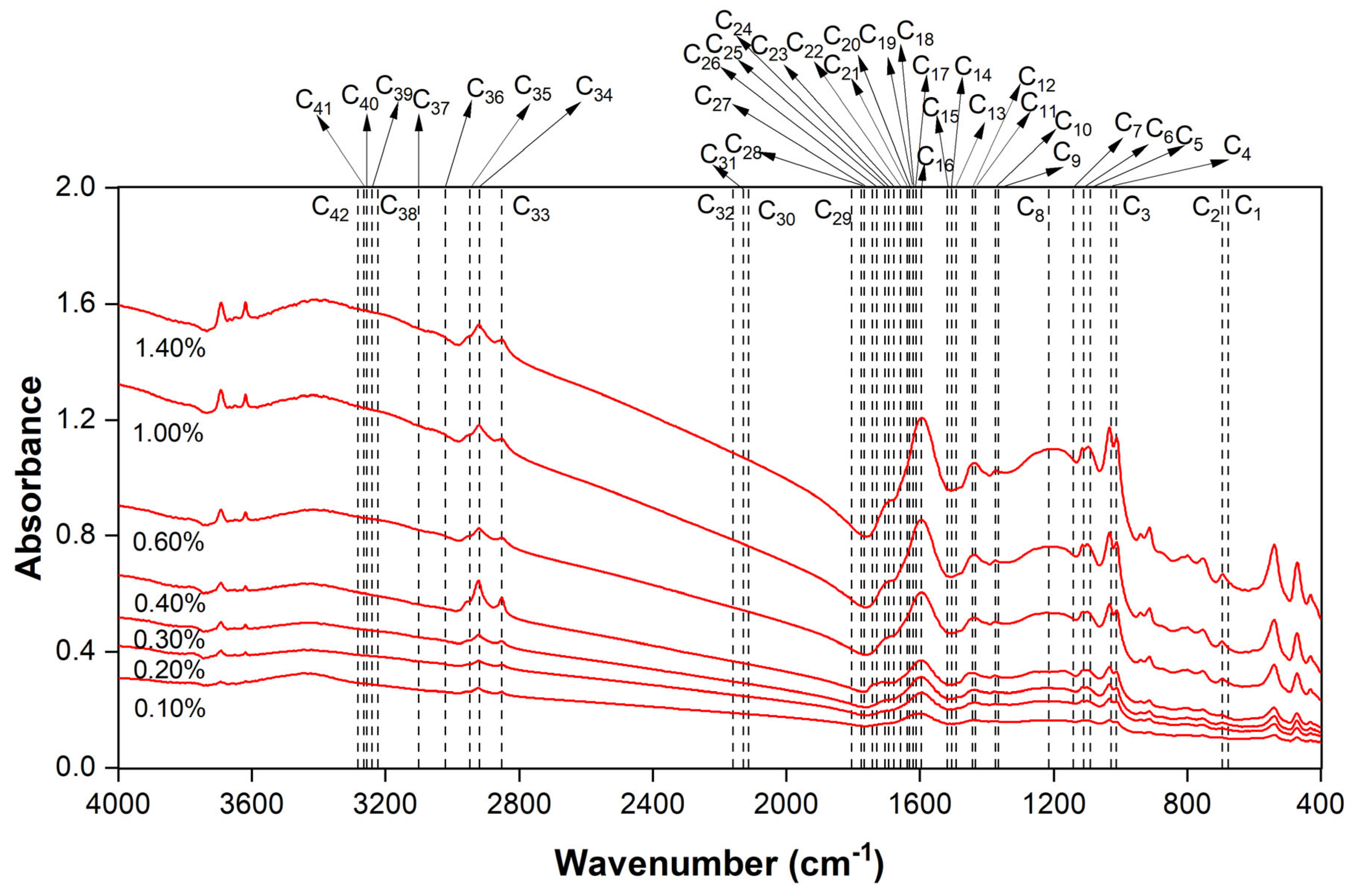
To study the nature of absorbance with respect to the carbon content at specific wavelengths, the pellets were prepared for FTIR analysis, as given below. Each coal sample was mixed with a laboratory-grade KBr powder to produce a set of seven Coal+KBr pellets with a specific dilution factor. The KBr amount was fixed at 220 ± 0.20 mg with varying coal content such that the content of the coal in the Coal+KBr mix (pellets) was at nearly 0.10, 0.20, 0.30, 0.40, 0.60, 1.00, and 1.40 percent. The spectral signature (absorbance) from each pellet was recorded, adjusted for baseline, and clipped for the wavenumber 4000–400 cm−1 range (Figure 3). The recorded signatures also include the spectra of KBr, which was added to the coal samples to make pellets. To remove the KBr signature, a spectral signature of only KBr pellets was recorded, and it was used as a baseline spectrum for further analysis. This baseline spectrum was subtracted from each pellet’s signature, and the resultant spectrum was used for further calculations.

3.3. Model Estimation

For model building and validation, the carbon content in the coal samples obtained through the traditional CHNS analyzer (CCHNS) was used as a reference (true value). For model development and validation, the training set and test set were formed using a 17:1 split (K-fold cross validation). The non-linear and linear relationships between the functional groups of carbon compounds (Table 2) that directly correspond with their amounts in the coal samples were modeled using a numerical iterative method based on the QN method with the breakpoint and loss function. The piecewise linear regression method employing the QN method with breakpoint was used with the objective of minimizing the difference between the predicted and observed values (the least squares loss function) and restricting the errors in the carbon estimation.
The model creates two distinct forms of the coefficient for the given variables (left and right equations, QNbp_L and QNbp_R) while considering the breakpoint and a single form of the coefficient (QNnbp) for the non-breakpoint. It has been found that the C% estimated from the avg equation (QNbp_avg, where bp = with breakpoint and avg = average of left and right equations) may offer the estimated value that is closest to the experimentally observed value.
Occasionally, as compared to experimental data, QNbp_avg estimates C% values that are outside of the expected range. Thus, the valid range, which is 1.5*IQR (interquartile range, IQR) and is derived using the QNbp_avg, was calculated in order to identify and eliminate out-of-range values (if any). As a result, if the anticipated value of the C% from QNbp_avg is out of range, the C% from QNnbp is considered the model’s estimated value. The overall efficacy of the FTIR-based estimation of C% is increased by employing a threshold to identify occasional out-of-range values, and it helps to reduce the error in estimating the carbon content in unknown samples. The procedure is demonstrated by the conditions described below:
Condition 1: The value from the QNbp_avg model is taken into consideration if the predicted carbon content (CFTIR, wt.% from QNbp_avg) is within the range (out min to out max):
Value within the range = QNbp_avg
Condition 2: The value from the QNnbp model is taken into consideration if the predicted carbon content (CFTIR, wt.% from QNbp_avg) is outside the range (out min to out max):
Value within the range = QNnbp
where:
Range = out min to out max (Q1 − (IQR × 1.5) to Q3 + (IQR × 1.5));
QNbp_avg = (QNbp_L + QNbp_R)/2;
QNbp_L = left equation from QNbp model;
QNbp_R = right equation from QNbp model;
QNnbp = QN model without breakpoint.
FTIR data containing the response spectra of assigned functional groups for the carbon compounds were utilized to run a thorough statistical analysis to evaluate the performance of the proposed model. The standard formulas were used to determine the measures of central tendency (Mean), measures of dispersion (SD), measures of systematic error (MBE), measures of the magnitude of error (MAE), and measures of dispersion in residuals (RMSE) [42].
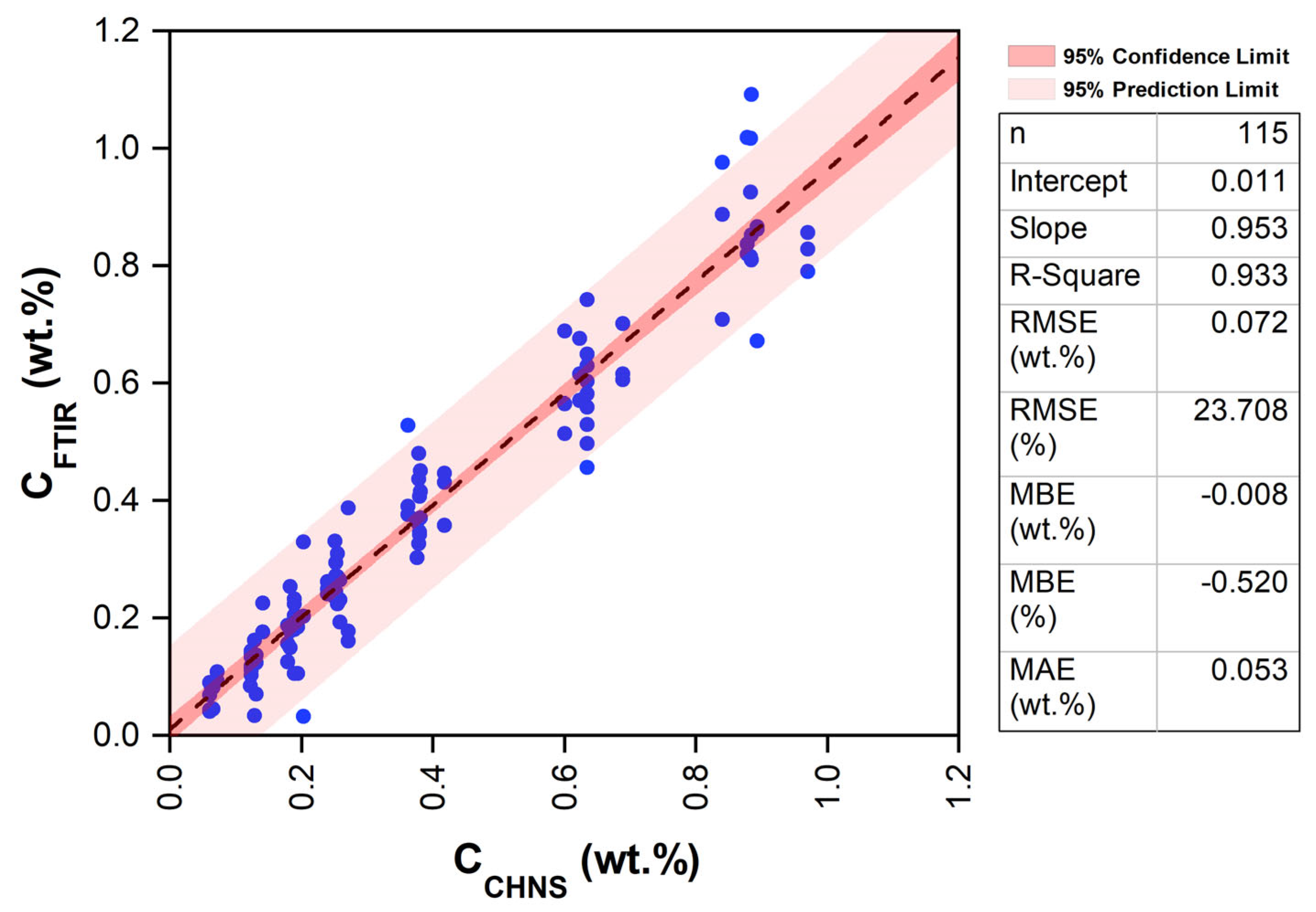
In Figure 4, the scatterplot of the observed carbon (CCHNS, wt.%) using CHNS data and the model-predicted carbon (CFTIR, wt.%) using FTIR data shows a strong linear relationship between them because of a good coefficient of determination (R2 = 0.93) and lower RMSE (0.072, wt.%), RMSE (23.71%), MBE (−0.52%), and MAE (0.053, wt.%).
However, as shown in the boxplot (Figure 5), the interquartile range and mean demonstrate that the carbon content estimated via the traditional (ultimate analysis) method and the proposed (FTIR spectroscopy) methodology are similar in range. The RMSE (23.71%), and MBE (−0.520%) are significantly low, which is reflected in the distribution of the mean bias error (Figure 5), and the MBE (in wt.%) ranges from approximately −0.22 to 0.21.
The two-tailed paired t-test for the mean was conducted (Table 3) at the confidence level (CL) of 99% (where α= 0.01) to investigate the significant mean difference (μd) between the observed (CCHNS, wt.%) and model-predicted (CFTIR, wt.%) mean values.
For two-tailed paired t-test (for mean):
Null Hypothesis:  H0: μd = 0
Alternative Hypothesis: H₁: μd ≠ 0
A two-tailed F-test of variance (S2) was conducted at the CL of 99% (where α= 0.01) to investigate the significant difference between the variance obtained from observed (CCHNS, wt.%) and model-predicted (CFTIR, wt.%) values.
For the two-tailed paired F-test (for variance):
Null Hypothesis: H0: σ02 = σp2
Alternative Hypothesis: H₁: σo2 ≠ σp2
where CCHNS—experimental (observed) carbon using CHNS values; CFTIR—estimated (modeled) carbon using FTIR data; n—no. of samples; R-square—coefficient of determination; RMSE—root mean square error; MBE—mean bias error; MAE—mean absolute error; RPD—relative percent difference.
From the t-test, it can be inferred that the null hypothesis H0 is accepted. It is noticeable that the mean of the observed values (CCHNS, wt.%) is significantly similar to the mean of the model-predicted values (CFTIR, wt.%) at the 99% confidence level, where α = 0.01. Similarly, in the F-test, the null hypothesis H0 is accepted. According to this, the variance of the observed (CCHNS, wt.%) values ( σ o 2 ) is significantly similar to the variance of the model-predicted (CFTIR, wt.%) values ( σ p 2 ) at the 99% confidence level (where α = 0.01). The acceptance region (Fstat < Ftable) for the F-test at the 99% confidence level is 0.615 to 1.626.
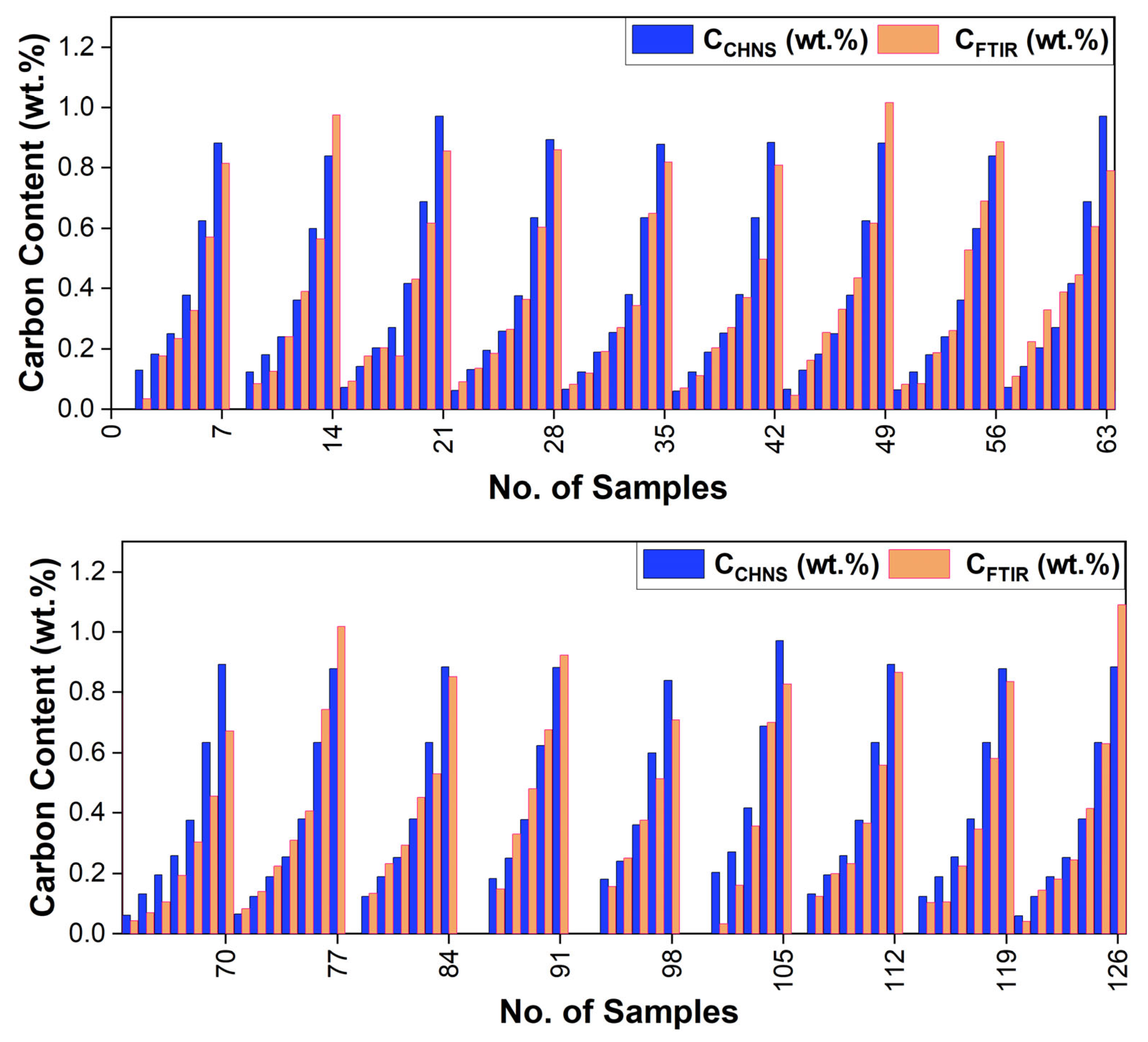
In Figure 6, the observed carbon content is plotted along with the model-predicted values. Each sample was divided into a set of seven for the analysis. A total of 115 samples were modeled, excluding the cases with negative anomalies in the FTIR values. The validation exercise using the independent test set clearly shows that the estimated modeled (using FTIR) values are nearly similar to their observed experimental (using ultimate analysis) values. Thus, the carbon content in the coal samples has been accurately predicted by the model employing FTIR spectral response.

3.4. Comparison with Previously Developed Models

A comparison between the previously published estimation methods and the present study for the determination of carbon content in coal samples is summarized in Table 4. In this table, the name of the method used in the estimation model, reference, location, nature, the number of samples, correlation statistics, and measures of error are tabulated for comparison.
In general, in terms of single point estimation, it was observed that the models using the LIBS estimation technique provide better correlation coefficients (R2 ranges from 0.86 to 0.99). LIBS provides a near-accurate value when targeting a single point-based estimation. The efforts to determine the elemental analysis of coal (C, H, N, and S) using data from the proximate analysis yielded a good correlation (R2 from 0.86 to 0.95) (Table 4). For bulk sample analysis, the current method using FTIR data gives a good correlation (correlation coefficient R2 = 0.93 compared to the ultimate analysis) with relatively low RMSE and bias (MBE). So, both the proposed method and the traditional method of ultimate analysis can accurately estimate the amount of carbon in large samples such as those from a specific coal seam (or a specific mine face, etc.).

4. Conclusions

Estimating the carbon content in coal is essential for determining its usability and the potential impact on health and the environment. The FTIR data-based model for estimating the amount of carbon in coal offers an alternative to traditional ultimate analysis with the CHNSO analyzer. The results of determining the carbon content using the FTIR-based model (CFTIR) are summarized as follows:
  • A strong linear relationship was found between the observed (CCHNS, wt.%) and model-estimated (CFTIR, wt.%) carbon content, with a high coefficient of determination (R2 of 0.93), low RMSE (23.71%), and low MBE (−0.52%).
  • The mean carbon contents estimated from CCHNS and CFTIR were 0.383 and 0.391, respectively. Similarly, the variance was 0.075 for the observed carbon using the CHNSO analyzer (CCHNS) and 0.077 for the FTIR data-based model (CFTIR).
  • The t-test and F-test of significance, conducted for mean and variance, respectively, clearly show that there is no significant difference between the CCHNS (wt.%, observed) and CFTIR (wt.%, model-estimated) values.
The authors recommend future research into calculating the carbon content in coal produced from various coal fields and basins using the proposed methodology based on the FTIR data. The FTIR data-based model has the potential to be further tested and employed in the regular determination of carbon in high-ash coal in laboratories and industries. The FTIR data-based model can also be suitably modified and tested to determine the carbon content in other types of natural samples, such as soil, shale, and other organic-rich rocks.

Author Contributions

Conceptualization, A.K.P.; methodology, A.K.P.; software, S.M., A.S., A.V. and A.K.P.; formal analysis, S.M., A.S., A.V. and A.K.P.; investigation, S.M., A.K.P. and K.P.; resources, A.K.P.; data curation, S.M.; writing—original draft preparation, S.M.; writing—review and editing, A.S., A.V., K.P., A.K.V. and A.K.P.; visualization, S.M.; supervision, A.K.P.; project administration, A.K.P.; funding/equipment acquisition: A.K.P. and A.K.V. All authors have read and agreed to the published version of the manuscript.

Funding

The research equipment (CHNS(O) analyzer and FTIR spectroscopy) was funded by DST, New Delhi, grant number DST-FIST Level-II Program (No. SR/FST/ESII-014/2012(C)).

Data Availability Statement

Not applicable.

Acknowledgments

The authors are thankful to South Eastern Coalfield Limited (SECL) for providing the necessary support related to the mine visit, sample collection, fieldwork, and geological literature. The authors are grateful to the DST, India (http://www.dst.gov.in), for providing financial support to set up the “DST-FIST Level-II Facility” at the Department of Applied Geology (AGL), IIT (ISM), Dhanbad (http://www.iitism.ac.in). For the sample preparation, analyses, and visualization used in this study, the authors are thankful to the AGL, IIT (ISM), Dhanbad, for providing the necessary access to the equipment (particularly the CHNS(O) analyzer and FTIR spectroscopy), technical support, and laboratory facilities through the DST-FIST Level-II Program (No. SR/FST/ESII-014/2012(C)). The authors are thankful to all of their colleagues and individuals who helped them directly or indirectly during the work.

Conflicts of Interest

The authors declare no conflict of interest.

References

  1. Saptoro, A.; Vuthaluru, H.B.; Tadé, M.O. A Comparative Study of Prediction of Elemental Composition of Coal Using Empirical Modelling. IFAC Proc. Vol. 2006, 39, 747–752. [Google Scholar] [CrossRef]
  2. Dmitrienko, M.A.; Strizhak, P.A. Coal-Water Slurries Containing Petrochemicals to Solve Problems of Air Pollution by Coal Thermal Power Stations and Boiler Plants: An Introductory Review. Sci. Total Environ. 2018, 613–614, 1117–1129. [Google Scholar] [CrossRef] [PubMed]
  3. Mcfarland, J.; Herzog, H.; Jacoby, H. The Future of Coal Consumption in a Carbon Constrained World. In Greenhouse Gas Control Technologies 7; Elsevier: Amsterdam, The Netherlands, 2005; Volume II, pp. 1563–1568. ISBN 978-0-08-044704-9. [Google Scholar]
  4. Yan, C.; Qi, J.; Ma, J.; Tang, H.; Zhang, T.; Li, H. Determination of Carbon and Sulfur Content in Coal by Laser Induced Breakdown Spectroscopy Combined with Kernel-Based Extreme Learning Machine. Chemom. Intell. Lab. Syst. 2017, 167, 226–231. [Google Scholar] [CrossRef]
  5. Li, X.; Yin, H.; Wang, Z.; Fu, Y.; Li, Z.; Ni, W. Quantitative Carbon Analysis in Coal by Combining Data Processing and Spatial Confinement in Laser-Induced Breakdown Spectroscopy. Spectrochim. Acta Part B At. Spectrosc. 2015, 111, 102–107. [Google Scholar] [CrossRef]
  6. Fowler, N.O.; McCall, D.; Chou, T.C.; Holmes, J.C.; Hanenson, I.B. Electrocardiographic Changes and Cardiac Arrhythmias in Patients Receiving Psychotropic Drugs. Am. J. Cardiol. 1976, 37, 223–230. [Google Scholar] [CrossRef] [PubMed]
  7. Noli, F.; Tsamos, P. Concentration of Heavy Metals and Trace Elements in Soils, Waters and Vegetables and Assessment of Health Risk in the Vicinity of a Lignite-Fired Power Plant. Sci. Total Environ. 2016, 563–564, 377–385. [Google Scholar] [CrossRef]
  8. Munawer, M.E. Human Health and Environmental Impacts of Coal Combustion and Post-Combustion Wastes. J. Sustain. Min. 2018, 17, 87–96. [Google Scholar] [CrossRef]
  9. Cappelaere, P. Prolactin and breast cancers. Pathol. Biol. 1975, 23, 161–170. [Google Scholar]
  10. Badman, D.G.; Jaffé, E.R. Blood and Air Pollution; State of Knowledge and Research Needs. Otolaryngol. Neck Surg. 1996, 114, 205–208. [Google Scholar] [CrossRef]
  11. Yi, L.; Feng, J.; Qin, Y.-H.; Li, W.-Y. Prediction of Elemental Composition of Coal Using Proximate Analysis. Fuel 2017, 193, 315–321. [Google Scholar] [CrossRef]
  12. Liu, F. A Comparison between Multivariate Linear Model and Maximum Likelihood Estimation for the Prediction of Elemental Composition of Coal Using Proximate Analysis. Results Eng. 2022, 13, 100338. [Google Scholar] [CrossRef]
  13. Čechák, T.; Thinová, L. Sulfur Content Measurement in Coal by X-Ray Fluorescence Method. Radiat. Phys. Chem. 2001, 61, 759–761. [Google Scholar] [CrossRef]
  14. Suarez-Fernandez, G.P.; Vega, J.M.G.; Fuertes, A.B.; Garcia, A.B.; Martinez-Tarazona, M.R. Analysis of Major, Minor and Trace Elements in Coal by Radioisotope X-Ray Fluorescence Spectrometry. Fuel 2001, 80, 255–261. [Google Scholar] [CrossRef]
  15. Pereira, J.S.F.; Mello, P.A.; Moraes, D.P.; Duarte, F.A.; Dressler, V.L.; Knapp, G.; Flores, É.M.M. Chlorine and Sulfur Determination in Extra-Heavy Crude Oil by Inductively Coupled Plasma Optical Emission Spectrometry after Microwave-Induced Combustion. Spectrochim. Acta Part B At. Spectrosc. 2009, 64, 554–558. [Google Scholar] [CrossRef]
  16. Chaves, E.S.; de Loos-Vollebregt, M.T.C.; Curtius, A.J.; Vanhaecke, F. Determination of Trace Elements in Biodiesel and Vegetable Oil by Inductively Coupled Plasma Optical Emission Spectrometry Following Alcohol Dilution. Spectrochim. Acta Part B At. Spectrosc. 2011, 66, 733–739. [Google Scholar] [CrossRef]
  17. Boulyga, S.F.; Heilmann, J.; Prohaska, T.; Heumann, K.G. Development of an Accurate, Sensitive, and Robust Isotope Dilution Laser Ablation ICP-MS Method for Simultaneous Multi-Element Analysis (Chlorine, Sulfur, and Heavy Metals) in Coal Samples. Anal. Bioanal. Chem. 2007, 389, 697–706. [Google Scholar] [CrossRef]
  18. Weritz, F.; Ryahi, S.; Schaurich, D.; Taffe, A.; Wilsch, G. Quantitative Determination of Sulfur Content in Concrete with Laser-Induced Breakdown Spectroscopy. Spectrochim. Acta Part B At. Spectrosc. 2005, 60, 1121–1131. [Google Scholar] [CrossRef]
  19. Gaft, M.; Nagli, L.; Fasaki, I.; Kompitsas, M.; Wilsch, G. Laser-Induced Breakdown Spectroscopy for on-Line Sulfur Analyses of Minerals in Ambient Conditions. Spectrochim. Acta Part B At. Spectrosc. 2009, 64, 1098–1104. [Google Scholar] [CrossRef]
  20. Yang, X.; Ingham, D.; Ma, L.; Srinivasan, N.; Pourkashanian, M. Ash Deposition Propensity of Coals/Blends Combustion in Boilers: A Modeling Analysis Based on Multi-Slagging Routes. Proc. Combust. Inst. 2017, 36, 3341–3350. [Google Scholar] [CrossRef]
  21. Qin, H.; Lu, Z.; Yao, S.; Li, Z.; Lu, J. Combining Laser-Induced Breakdown Spectroscopy and Fourier-Transform Infrared Spectroscopy for the Analysis of Coal Properties. J. Anal. At. Spectrom. 2019, 34, 347–355. [Google Scholar] [CrossRef]
  22. Yao, S.; Qin, H.; Wang, Q.; Lu, Z.; Yao, X.; Yu, Z.; Chen, X.; Zhang, L.; Lu, J. Optimizing Analysis of Coal Property Using Laser-Induced Breakdown and near-Infrared Reflectance Spectroscopies. Spectrochim. Acta. A. Mol. Biomol. Spectrosc. 2020, 239, 118492. [Google Scholar] [CrossRef]
  23. Gazeli, O.; Stefas, D.; Couris, S. Sulfur Detection in Soil by Laser Induced Breakdown Spectroscopy Assisted by Multivariate Analysis. Materials 2021, 14, 541. [Google Scholar] [CrossRef] [PubMed]
  24. Solomon, P.R.; Serio, M.A.; Carangelo, R.M.; Bassilakis, R.; Gravel, D.; Baillargeon, M.; Baudais, F.; Vail, G. Analysis of the Argonne Premium Coal Samples by Thermogravimetric Fourier Transform Infrared Spectroscopy. Energy Fuels 1990, 4, 319–333. [Google Scholar] [CrossRef]
  25. Ahmed, M.A.; Blesa, M.J.; Juan, R.; Vandenberghe, R.E. Characterisation of an Egyptian Coal by Mossbauer and FT-IR Spectroscopy. Fuel 2003, 82, 1825–1829. [Google Scholar] [CrossRef]
  26. Kaihara, M.; Takahashi, T.; Akazawa, T.; Sato, T.; Takahashi, S. Application of Near Infrared Spectroscopy to Rapid Analysis of Coals. Spectrosc. Lett. 2002, 35, 369–376. [Google Scholar] [CrossRef]
  27. Orrego-Ruiz, J.A.; Cabanzo, R.; Mejía-Ospino, E. Study of Colombian Coals Using Photoacoustic Fourier Transform Infrared Spectroscopy. Int. J. Coal Geol. 2011, 85, 307–310. [Google Scholar] [CrossRef]
  28. Ghosh, A.K.; Tewari, R.; Agnihotri, D.; Kar, R.; Pillai, S.S.K.; Bajpai, S.; Tripathi, S.C. Field Guide Book: Gondwana Formations of South Rewa and Upper Narmada Basins, Central India; Birbal Sahni Institute of Palaeobotany: Lucknow, India, 2015; p. 40. [Google Scholar]
  29. Mukherjee, D.; Ray, S.; Chandra, S.; Pal, S.; Bandyopadhyay, S. Upper Gondwana Succession of the Rewa Basin, India: Understanding the Interrelationship of Lithologic and Stratigraphic Variables. J. Geol. Soc. India 2012, 79, 563–575. [Google Scholar] [CrossRef]
  30. Dutta, P.K.; Acharyya, S.K.; Jha, N.; Khangar, R.; Khasdeo, L.; Misra, K.G.; Ramanamurty, B.V. Resolving Kamthi-Related Problems in Gondwana Stratigraphy of Peninsular India. Indian J. Geosci. 2015, 69, 85–102. [Google Scholar]
  31. ASTM D2234/D2234M−17 2017; American Society for Testing and Materials (ASTM) Standard Practice for Collection of a Gross Sample of Coal. ASTM: Philadelphia, PA, USA, 2017.
  32. ASTM D4749−12 2012; American Society for Testing and Materials (ASTM) Standard Test Method for Performing the Sieve Analysis of Coal and Designating Coal Size. ASTM: Philadelphia, PA, USA, 2012.
  33. ASTM D5373−16 2016; American Society for Testing and Materials (ASTM) Standard Test Methods for Determination of Carbon, Hydrogen and Nitrogen in Analysis Samples of Coal and Carbon in Analysis Samples of Coal and Coke. ASTM: Philadelphia, PA, USA, 2016.
  34. ASTM D4239−18 2018; American Society for Testing and Materials (ASTM) Standard Test Method for Sulfur in the Analysis Sample of Coal and Coke Using HighTemperature Tube Furnace Combustion. ASTM: Philadelphia, PA, USA, 2018.
  35. Organic Elemental Analyzer Vario MACRO Cube—Elementar. Available online: https://www.elementar.com/en-in/products/organic-elemental-analyzers/vario-macro-cube (accessed on 15 February 2023).
  36. Othman, N. IR Spectroscopy in Qualitative and Quantitative Analysis. In Infrared Spectroscopy-Perspectives and Applications; IntechOpen: London, UK, 2022. [Google Scholar]
  37. Prasad, A.K.; Singh, R.P.; Tare, V.; Kafatos, M. Use of Vegetation Index and Meteorological Parameters for the Prediction of Crop Yield in India. Int. J. Remote Sens. 2007, 28, 5207–5235. [Google Scholar] [CrossRef]
  38. Singh, R.P.; Prasad, A.K.; Tare, V.; Kafatos, M. Crop Yield Prediction Using Piecewise Linear Regression with a Break Point and Weather and Agricultural Parameters. U.S. Patent No. 7,702,597, 20 April 2010. [Google Scholar]
  39. Speight, J.G. Handbook of Coal Analysis, 2nd ed.; Wiley: Hoboken, NJ, USA, 2015; ISBN 978-1-119-03832-0. [Google Scholar]
  40. Pavia, D.L.; Lampman, G.M.; Kriz, G.S.; Vyvyan, J.A. Introduction to Spectroscopy, 5th ed.; Cengage Learning: Boston, MA, USA, 2014; ISBN 978-1-305-17782-6. [Google Scholar]
  41. Stuart, B.H. Infrared Spectroscopy: Fundamentals and Applications; John Wiley & Sons: Hoboken, NJ, USA, 2004; ISBN 978-0-470-01113-3. [Google Scholar]
  42. Preety, K.; Prasad, A.K.; Varma, A.K.; El-Askary, H. Accuracy Assessment, Comparative Performance, and Enhancement of Public Domain Digital Elevation Models (ASTER 30 m, SRTM 30 m, CARTOSAT 30 m, SRTM 90 m, MERIT 90 m, and TanDEM-X 90 m) Using DGPS. Remote Sens. 2022, 14, 1334. [Google Scholar] [CrossRef]
  43. Zhang, Y.; Dong, M.; Cheng, L.; Wei, L.; Cai, J.; Lu, J. Improved Measurement in Quantitative Analysis of Coal Properties Using Laser Induced Breakdown Spectroscopy. J. Anal. At. Spectrom. 2020, 35, 810–818. [Google Scholar] [CrossRef]
  44. Dong, M.; Wei, L.; Lu, J.; Li, W.; Lu, S.; Li, S.; Liu, C.; Yoo, J.H. A Comparative Model Combining Carbon Atomic and Molecular Emissions Based on Partial Least Squares and Support Vector Regression Correction for Carbon Analysis in Coal Using LIBS. J. Anal. At. Spectrom. 2019, 34, 480–488. [Google Scholar] [CrossRef]
  45. Feng, J.; Wang, Z.; West, L.; Li, Z.; Ni, W. A PLS Model Based on Dominant Factor for Coal Analysis Using Laser-Induced Breakdown Spectroscopy. Anal. Bioanal. Chem. 2011, 400, 3261–3271. [Google Scholar] [CrossRef] [PubMed]
  46. Feng, J.; Wang, Z.; Li, L.; Li, Z.; Ni, W. A Nonlinearized Multivariate Dominant Factor–Based Partial Least Squares (PLS) Model for Coal Analysis by Using Laser-Induced Breakdown Spectroscopy. Appl. Spectrosc. 2013, 67, 291–300. [Google Scholar] [CrossRef] [PubMed]
  47. Xu, X.; Li, A.; Wang, X.; Ding, C.; Qiu, S.; He, Y.; Lu, T.; He, F.; Zou, B.; Liu, R. The High-Accuracy Prediction of Carbon Content in Semi-Coke by Laser-Induced Breakdown Spectroscopy. J. Anal. At. Spectrom. 2020, 35, 984–992. [Google Scholar] [CrossRef]
  48. Li, X.; Wang, Z.; Fu, Y.; Li, Z.; Ni, W. A Model Combining Spectrum Standardization and Dominant Factor Based Partial Least Square Method for Carbon Analysis in Coal Using Laser-Induced Breakdown Spectroscopy. Spectrochim. Acta Part B At. Spectrosc. 2014, 99, 82–86. [Google Scholar] [CrossRef]
  49. Wang, Z.; Yuan, T.-B.; Lui, S.-L.; Hou, Z.-Y.; Li, X.-W.; Li, Z.; Ni, W.-D. Major Elements Analysis in Bituminous Coals under Different Ambient Gases by Laser-Induced Breakdown Spectroscopy with PLS Modeling. Front. Phys. 2012, 7, 708–713. [Google Scholar] [CrossRef]
  50. Andrés, J.M.; Bona, M.T. Analysis of Coal by Diffuse Reflectance Near-Infrared Spectroscopy. Anal. Chim. Acta 2005, 535, 123–132. [Google Scholar] [CrossRef]
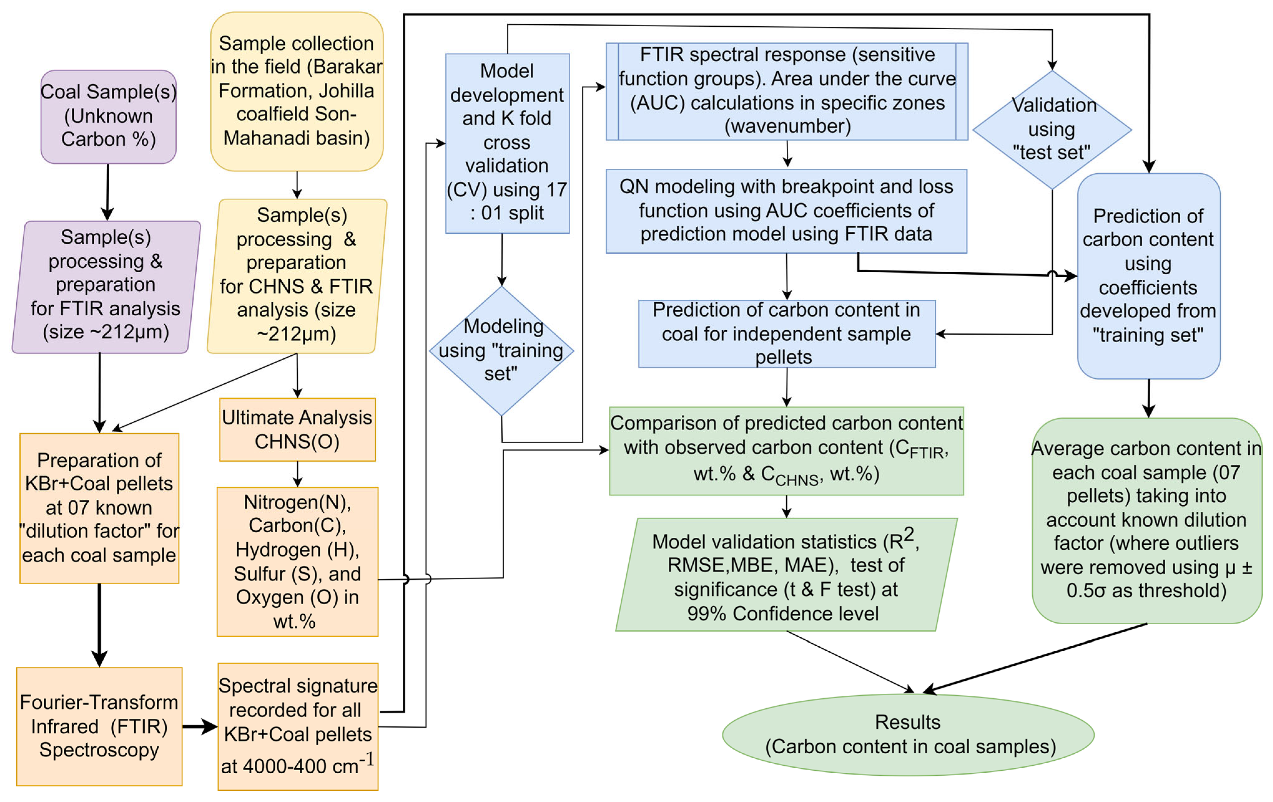
Figure 1. Flow chart demonstrating the processing steps of the carbon content prediction model used in this study. The thick and thin arrows mark specific flow paths.
Minerals 13 00938 g001
Figure 2. Location map of coal sampling sites on the geological map of study area (southern part of Umaria District, MP, India). Abbreviations: Qt—Quaternary, Ct—Cretaceous, L.—Lower, Ec—Eocene, Pr—Permian, PC—Pre-Cambrian, PZ—Proterozoic, MP—Madhya Pradesh.
Minerals 13 00938 g002
Figure 3. For a series of seven Coal+KBr pellets (for Johilla S07) made at 0.10, 0.20, 0.30, 0.40, 0.60, 1.00, and 1.40 percent of coal, a systematic increase in absorbance is clearly discernible using FTIR spectroscopy. The location of peaks for sensitive/functional groups related to carbon in coal is marked in series from C1, C2, …, C42 (as given in Table 2).
Minerals 13 00938 g003
Figure 4. Scatter plot depicting the correlation between the observed (using ultimate analysis) and model-estimated (using FTIR) carbon values, along with the measures of error.
Minerals 13 00938 g004
Figure 5. (a) Boxplot for the comparison between the estimation of the carbon content in coal using CHNSO analyzer (CCHNS) and FTIR-based model (CFTIR). (b) Distribution of the mean bias error (MBE) for CFTIR using CCHNS as true values.
Minerals 13 00938 g005
Figure 6. Comparison between the carbon content for observed (ultimate analysis) and model-predicted (FTIR) (coal) samples.
Minerals 13 00938 g006
Table 1. Elemental composition of coal samples from the Johilla coalfield, Son-Mahanadi Basin, Madhya Pradesh, India, based on the ultimate analysis of coal using the CHNSO analyzer and ash yield using proximate analysis.
SampleUltimate Analysis (wt.%)
NadCadHadSadOdifAshad
Johilla_S011.2965.294.150.8328.458.40
Johilla_S021.1253.383.545.7136.2512.20
Johilla_S031.3267.983.562.1924.959.20
Johilla_S041.1863.923.891.3529.6617.50
Johilla_S051.2663.833.820.7430.3513.00
Johilla_S061.3559.383.611.5734.1013.00
Johilla_S071.3963.803.840.7230.2610.30
Johilla_S081.0961.063.840.7033.319.40
Johilla_S091.2868.893.510.9625.369.50
Johilla_S101.1756.423.861.0137.5410.30
Johilla_S111.3664.533.770.6429.7017.80
Johilla_S121.3959.603.531.6733.805.00
Johilla_S131.2862.984.040.7830.929.80
Johilla_S141.2560.143.660.7234.2310.40
Johilla_S151.2368.953.502.1924.1311.10
Johilla_S161.0664.104.100.7030.0411.70
Johilla_S171.2963.253.780.6231.0612.00
Johilla_S181.2663.323.530.9230.9711.40
Mean1.2562.823.751.3330.8411.22
Med1.2763.563.780.8830.6410.75
SD0.104.040.211.203.682.99
Var0.0116.350.041.4513.568.96
Min1.0653.383.50.6224.135.00
Max1.3968.954.155.7137.5417.80
Explanation: N—nitrogen (wt.%), C—carbon (wt.%), H—hydrogen (wt.%), O—oxygen (wt.%), S—sulfur (wt.%), ad—as determined basis, diff—calculated by difference.
Table 2. Assigned band details concerning the functional groups of the carbon compound used in the study, modified after [40,41].
PeaksCenterStartEndFunctional Group and Nature of Bond
C1671.33664.192674.19Mercaptans and thioethersC-S
C2694.187674.19718.47
C31011.2851001.2871021.284Alcohols, ethers, esters, carboxylic acids, anhydridesC-O
C41032.7111021.2841069.849
C51099.8441069.8491108.415
C61114.1281108.4151138.41
C71164.1211138.411179.833
C81229.8261179.8331299.816
C91368.3781359.8081374.091Alkanes-CH3
C101378.3771374.0911385.518
C111451.2231445.511456.937Alkanes and aromaticH-C-H & C-C=C
C121462.651456.9371472.649
C131492.6461486.9331495.503
C141501.2161495.5031505.501
C151512.6431505.5011518.357
C161598.3461585.491608.344Alkenes and amidesC-C=C &C=O
C171611.2011608.3441615.486
C181619.7711615.4861624.056
C191628.3411624.0561634.055Amide, ketones, aldehydes, carboxylic acids, esterC=O
C201638.341634.0551648.338
C211652.6241648.3381671.192
C221675.4771671.1921682.619
C231691.191682.6191696.903
C241701.1881696.9031716.9
C251721.1851716.91732.612
C261736.8971732.6121748.324
C271775.4631769.751779.748Anhydrides and acyl halidesC=O
C281785.4621779.7481791.175
C291802.6021791.1751808.316
C302115.4152108.2742119.701AlkyneC≡C
C312136.8412128.2712142.554
C322162.5522156.8382165.408
C332851.0262821.3032876.737AlkanesH-C-H
C342921.0162876.7372948.155
C352958.1542948.1552982.436
C363040.9993008.1473072.423Alkenes and aromaticC=C-H
C373100.9913072.4233129.558
C383219.5453205.2623223.831Alkynes≡C-H
C393233.8293223.8313239.543
C403245.2563239.5433250.97
C413255.2553250.973263.825
C423275.2523263.8253282.394
Table 3. Results of two-tailed paired t- (and F-) test for comparison of the difference in the mean (and variance) of carbon content obtained via observed (CCHNS, wt.%) and model-estimated values (CFTIR, wt.%) at 99% confidence level and α= 0.01.
Pair x ¯ S2ndft-TestF-Test
tstatp-ValuetcriticalH0: μd = 0Fstatp-ValueCIH0: σo2p2
CFTIR (wt.%)0.3910.0771151141.1390.2572.620T1.0270.887(0.615–1.626)T
CCHNS (wt.%)0.3830.075
Explanation, x ¯ —mean, S2—sample variance, n—no. of observations, df—degree of freedom, tstat—t-statistic, tcritical—critical value of two-tailed paired t-test, μd—hypothesized mean difference, Fstat—F-statistic, p-value—probability distribution for two-tailed t- and F-test, CI—confidence interval, CL—confidence level, α—level of significance, T—true, F—false.
Table 4. Comparison between the methods for estimating carbon content in coal in previous studies and in the present study.
Sl. No.MethodSample Location [Reference]Nature;
Number of Samples
R2RMSE,
(MBE)
1Correlation with proximate analysisChina
[11]
Lignite;
N= 66
0.92NA
Sub-bituminous;
N= 74
0.86NA
Bituminous;
N= 94
0.93NA
Anthracite;
N= 66
0.95NA
2Correlation with proximate analysis (MLM)China
[12]
Coal (blend);
N = 755
NA2.72,
(0.26%)
Correlation with proximate analysis (MLE)NA1.91,
(0.63%)
3LIBS with SVRChina
[43]
Coal;
N = 44
0.991.08%,
NA
4LIBS with MLR and SVRChina
[44]
Coal;
N = 44
0.991.43%,
NA
LIBS with MLR and PLSR0.992.46%,
NA
LIBS with MLR0.863.41%,
NA
5LIBS with PLS based on dominant factorChina
[45]
Bituminous;
N = 33
0.994.47%,
NA
6LIBS with nonlinearized multivariate dominant factorChina
[46]
Bituminous;
N = 33
0.943.28%,
NA
LIBS with nonlinearized multivariate dominant factor-based PLS0.973.13%,
NA
7LIBS with PLS–SVMChina
[47]
Bituminous (semi coke);
N = 79
0.940.90%,
NA
8LIBS with K-ELMChina
[4]
Coal;
N = 26
0.990.37,
NA
9LIBS with spectrum standardization and dominant factor-based PLS with spatial confinementChina
[48]
Bituminous;
N = 24
0.991.35%,
(-)
10LIBS with PLS (Ambience: Air)China
[49]
Bituminous;
N = 24
0.873.91%,
(-)
LIBS with PLS (Ambience: Ar)0.952.69%,
(-)
LIBS with PLS (Ambience: He)0.962.43%,
(-)
11DRIFTS and NIRS with PCAGermany, Poland, Czech Republic, Russia, China, North-America, Australia, and Spain
[50]
Coal (blend);
N = 142
-2.58%,
(-)
12FTIR with QNJohilla, India
[Present Study]
Coal;
N = 115
0.9323.71%,
(−0.52%)
Note: R2—coefficient of determination, RMSE—root mean square error, ABE—average biased error, MBE—mean bias error, NA—not available.
Disclaimer/Publisher’s Note: The statements, opinions and data contained in all publications are solely those of the individual author(s) and contributor(s) and not of MDPI and/or the editor(s). MDPI and/or the editor(s) disclaim responsibility for any injury to people or property resulting from any ideas, methods, instructions or products referred to in the content.