Article

Parameterization of Multi-Angle Shaker Based on PSO-BP Neural Network

1
College of Mining Engineering, North China University of Science and Technology, Tangshan 063210, China
2
Collaborative Innovation Center of Green Development and Ecological Restoration of Mineral Resources, Tangshan 063210, China
3
Tangshan Land Sky Tech Co., Ltd., Tangshan 063020, China
*
Author to whom correspondence should be addressed.
Minerals 2023, 13(7), 929; https://doi.org/10.3390/min13070929
Submission received: 25 June 2023 / Revised: 8 July 2023 / Accepted: 10 July 2023 / Published: 11 July 2023
(This article belongs to the Section Mineral Processing and Extractive Metallurgy)

Abstract

:
It was possible to conduct a study on the shape and parameterization of the vibrating screen so as to explore the relationship between detailed vibrating screen motion parameters and particle group distribution under different screen surface states. The motion characteristics of particle groups in various scenes were investigated, screening performance of vibrating screen with complex parameters was studied, interaction between motion parameters of screen surface and motion of material groups in multi-component mixed particle groups was analyzed, segregation distribution law of multi-component mixed material groups was revealed, and this study presents simulation findings based on the discrete element program EDEM. The ensemble learning approach was used to examine the optimized model screen. It was revealed that the screen’s amplitude, vibration frequency, vibration direction angle, swing frequency, swing angle, and change rate of screen surface inclination all had a major impact on its performance. As a result, the vibrating screen’s running state was described by various parameter combinations, and the trend changes of several factors that affected the performance of the screen were examined. The investigation revealed that the particle swarm optimization backpropagation (PSO-BP) neural network model outperformed the backpropagation (BP) neural network model alone in terms of prediction. It had lower root mean square error (RMSE), mean square relative error (MSRE), mean absolute error (MAE), and mean absolute relative error (MARE) than the BP neural network model, but a larger R2. This model’s greatest absolute error was 0.0772, and its maximum relative error was 0.0241. The regression coefficient R value of 0.9859, which displayed the model’s strong performance and high prediction accuracy, showed that the PSO-BP model was feasible and helpful for parameter optimization design of vibrating screens.

1. Introduction

A vibrating screen is a commonly used piece of equipment for particle separation in bulk materials, which is widely used in mining, agriculture, and food fields [1,2,3]. The vibrating screen is welcomed by the majority of front-line workers because of its simple design, wear-resistant and durable, and the vibrating screen’s performance is critical to the quality of product manufacture; many researchers used a variety of ways to carry out parametric research on the vibrating screen, and achieved a series of scientific research results. Chen Z et al. [4] obtained the optimal screen surface inclination angle of different screen surface morphology by adjusting different screen surface parameters and using different mismatch proportion material groups for experiments. Based on the challenge of challenging monitoring inside the closed screen body, Wang et al. [5] suggested an improved YOLOv5 monitoring method. The method increased the accuracy of internal information monitoring in the interior region of the screen machine based on the fluid motion characteristics of the screen surface and produced considerable improvement in monitoring accuracy at a reasonable cost. Aghlmandi Harzanagh Ahad [6] established a differential equation for the dynamics of the center of mass of a single particle and proposed a single particle mechanical model in a complex environment; the migration velocity and change rule of the screen surface region in a complex environment were acquired using a high-speed dynamic camera as a carrier to investigate the state of the screen surface under varied load situations. Lin et al. performed material study using a stiff flexible coupling multibody system to improve wet material dehydration and classification. They conducted dynamic studies on the effects of processed materials on the damping and stiffness of the screen surface, showing the dynamic features of the screen surface as well as the material’s sensitivity throughout the screening process [7].
EDEM is widely used in simulation of loose materials due to its excellent adaptability. It can not only record the stress process between bulk materials but also track and analyze individual materials to record and describe the movement of the overall system material group. Therefore, the research of complex environments and screening mechanisms in multiple scenarios using EDEM discrete element method was a hot topic in the screening field for a long time [8]. In discrete element simulation, the most widely used model is Hertz-Mindlin (no slip). As it covered a variety of forces during the screening process, including commonly used static and dynamic friction, tangential force, collision recovery force, etc., it is widely used in the contact model setting of bulk materials, and the contact model and force type of materials are important factors affecting the movement of materials. As a result, fine-quantifying performance indicators such as force range and material type between materials are required to correctly affect the interaction between various components in order to evaluate the microscopic mechanism of particle groups [9]. Xiao J [10] refined and adjusted the geometric parameters of the double-layer multi-stage variable inclination screen surface, and optimized the screening efficiency and processing capacity of the material group with different parameters as the optimization objective to obtain the correlation formula between the acceleration of different screen surfaces and the material group, which provided the optimization basis for the screen machine structure and the process man. In addition to external circumstances such as screen machine specifications, the form features of the material and the feed rate have a significant impact on the screening effect. In addition to the external conditions such as the parameters of the screen machine, the shape characteristics of the material and the feed rate also have an important influence on the screening effect. Xia X et al. [11] verified the importance of material shape characteristics for screening simulation by studying variable factors such as feed rate and screen aperture, and conducting simulation analysis with spherical shape and simulated particle shape.
Most studies aimed to look into the effect of single parameter modifications on vibrating displays, generally focused on the interplay of single or multiple parameters. For example, Zhao et al. [12] used neural networks to investigate the distribution law of materials under various vibration parameters, studied the particle screening process and its distribution status, but failed to investigate the combination of motion parameters and the variable inclination gradient changes of the screen surface. This article used the three-dimensional discrete element program EDEM to simulate the screening process in various scenarios based on screening dynamics. The study focused on the variations in the motion parameters of the screen surface and the gradient of the form variations. In order to accurately analyze the effects of different amplitudes, vibration frequencies, vibration direction angles, swing frequencies, swing angles, and screen surface inclination changes on the performance of the screening machine, the PSO-BP neural network was used to map and describe various complex nonlinear parameters, thus reasonably adjusting the process configuration of the vibrating screen, optimizing parameter configuration, and improving the screening mechanism of the device [13].

2. Establishment of Vibrating Screen Model and Evaluation of Screen Performance

2.1. EDEM Model Machine and Simulation Parameters

As the most used discrete element software for force changes and motion trajectory changes of loose materials, EDEM can intuitively understand the motion laws of particle groups in screening, to conduct performance research on vibrating screens under solid works. As a result, the model was created using the three-dimensional modeling program SlideWorks, and the simplified model of the vibrating screen was turned into a stl file and put into EDEM software (version: 2022) for numerical calculation. The model is shown in Figure 1.
To ensure the computer processing ability and complexity of the components of the sieve machine during the simulation process, only the three major parts of the sieve box, sieve surface, and feeding port of the sieve machine are retained in the establishment of the sieve machine model, and complex screening scenarios under various working conditions were reproduced. The simplified model machine screen surface were formed by splicing five small screens with a length of 32 mm and a width of 30.5 mm. The gradient of the inclination angle of each screen surface was adjusted to 5°, at which point the inclination angle of the screen surface were 0, 5, 10, 15, and 20°. To meet the structural strength of the screen surface and to achieve efficient screening in complex environments of the screen machine, 304 stainless steel was selected as the screen surface material, and the side length of the screen surface was 3 × 3 mm2 square sieve hole processing. Finally, the size of the sieve box was modeled and the length, width, and height of the sieve box as were defined as 160 mm, 30.5 mm, and 80 mm, respectively. The size of the coarse material collection box was 30.5 × 30.5 mm2.
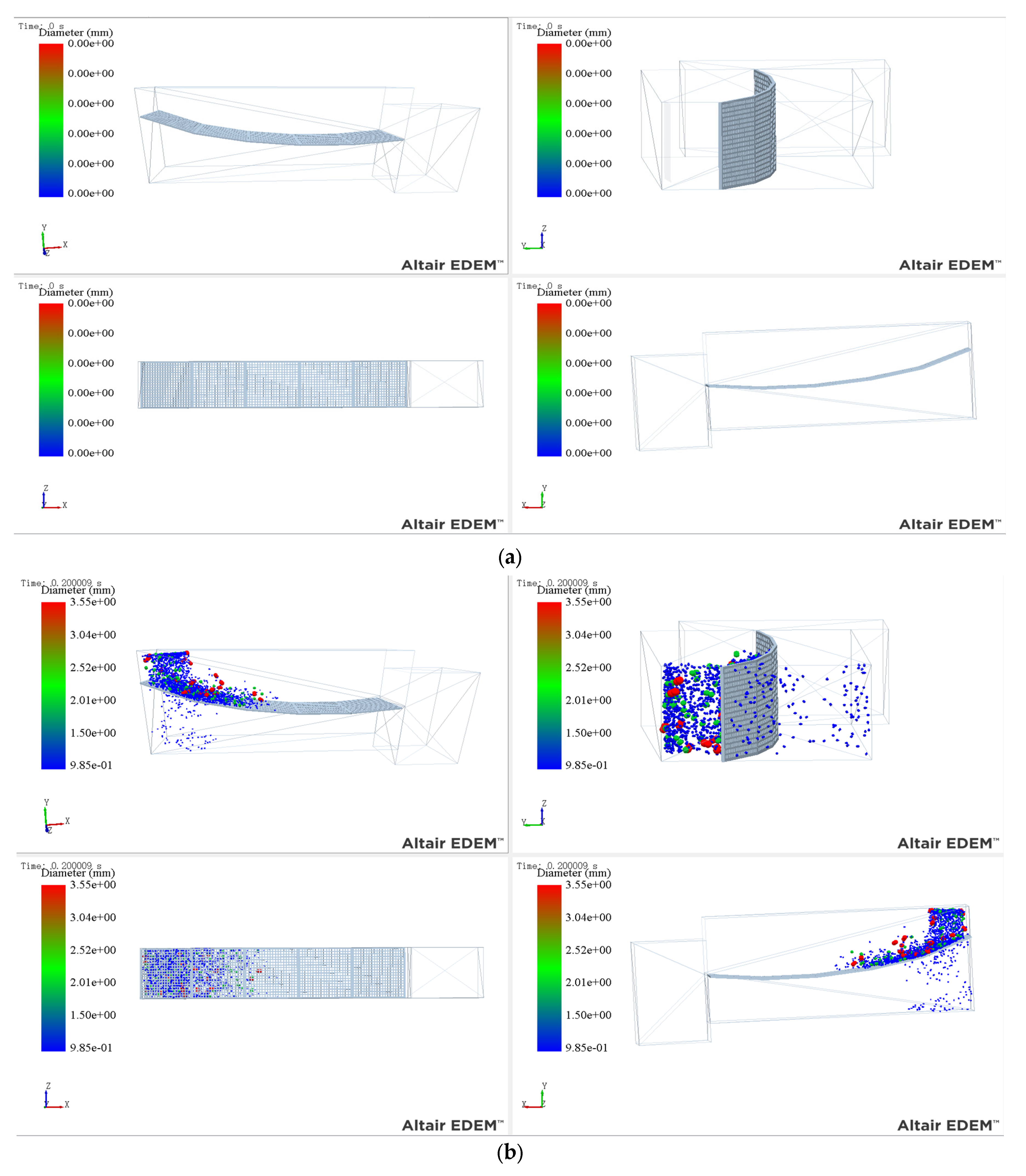
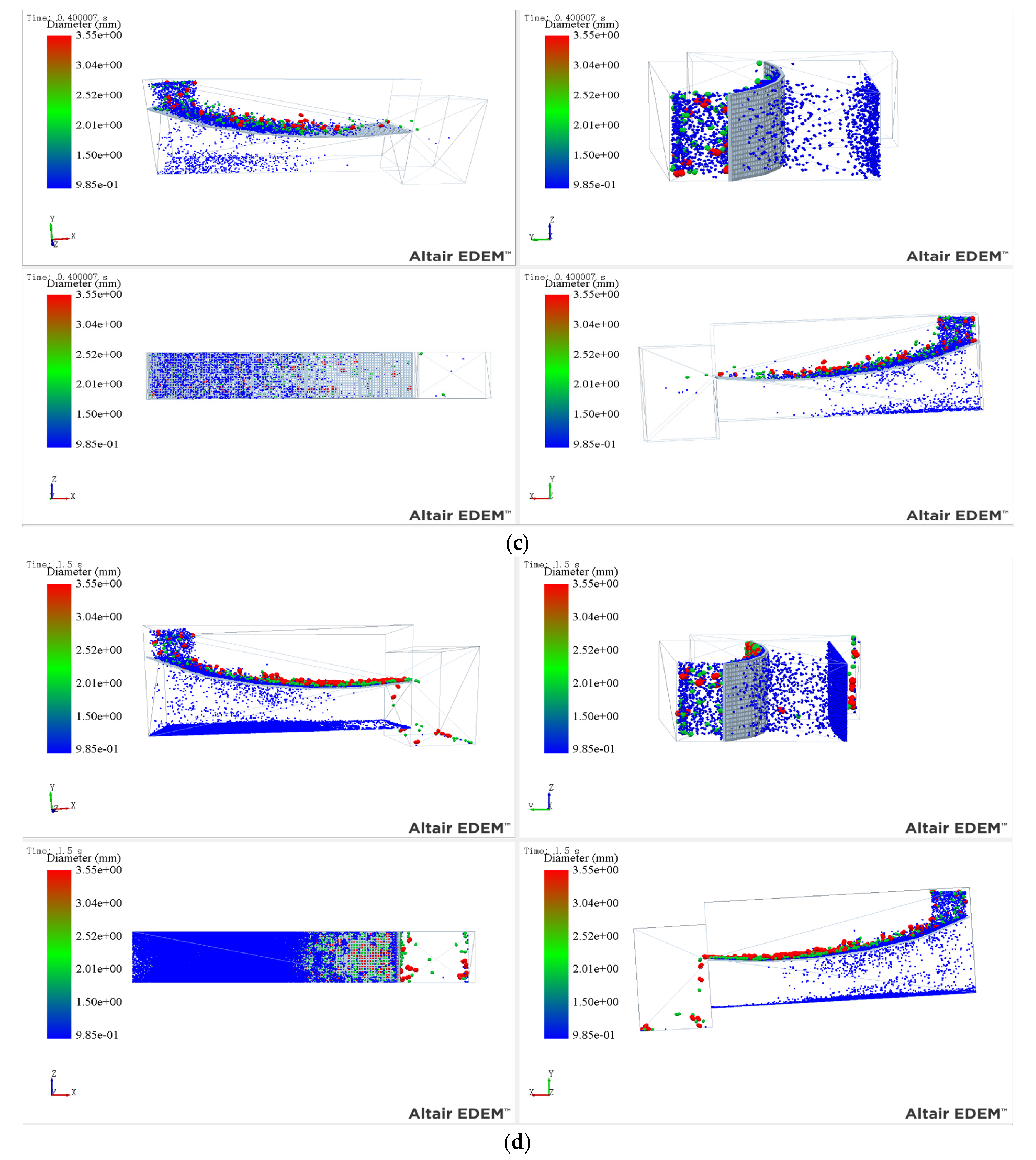
In Figure 2, the simulation procedure was displayed. Both the sieve machine’s feeding and the sieve body’s start time begin at 0 s. There was no variation in the particle size of the material body in the cloud picture at this point, as illustrated in Figure 2a, since the material body had not yet entered the sieve box. The material started to migrate on the screen surface after 0.2 s of feeding, and the screen machine operated smoothly under the excitation force. As illustrated in Figure 2b, a significant portion of the target materials in the material group were now moving under the coarse-grained material body without having yet pierced the screen. Some of the items had reached the edge of the screen surface after 0.4 s of the screening procedure. The grading impact had already started to become apparent, as indicated in Figure 2c, and it was discovered by the cloud map marking that there were almost no fine-grained materials in the material group at this time. The material on the screen stabilizes after 1.5 s of screening, and the process moves forward smoothly and steadily, as illustrated in Figure 2d.
The simulation parameters were adjusted to make the simulation screening process more representative and to verify that the simulation parameters not only suited the model but also matched the field prototype test findings. The material was set as continuous feed, the feed rate was 0.3 kg/s, the number of particle generation attempts was 20, and the feed composition was a bimodal normal distribution with an average particle size of 1.5 and 3 mm. The screen surface motion parameters were applied by presetting the motion behavior of the screen surface in EDEM, and the inclination of the screen surface was modified throughout the modeling process, to achieve the double-mode operation of the multi-angle screen machine under different parameters. The data of each object used in that simulation were obtained by look up relevant data, the material properties are shown in Table 1, and the collision characteristics are shown in Table 2.
The vibration intensity K [14] expressed the intensity of the movement of the target screening material on the screen surface:
K = A f 2 g sin β cos α
where A represents amplitude, mm; f stands for vibration frequency, Hz; g is the acceleration of gravity, m/s2; β is the vibration direction Angle, °; α is the inclination Angle of the screen surface, °.
The vibration frequency, amplitude, vibration direction angle, and inclination angle of each screen surface, as shown in Equation (1), have an effect on the vibration strength of the screen machine. Increased vibration frequency, for example, can increase the number of collisions between the screen surface and the material, the acquisition rate of kinetic energy of the material, and the number of jumping and the likelihood of material contact. Increased amplitude can accelerate the material’s loose rate, broaden the material’s space range of movement, and enhance the material’s blocking condition.

2.2. Screening Evaluation Criteria

In this work, EDEM software was used to model and evaluate the vibrating screen screening process. It was discovered that material larger than the screen hole could not pass through the screen surface and could not complete the sifting behavior by analyzing the definition of material particle material and screen surface attributes, so the extreme case of large particles passing through the screen surface was not considered. The screening effectiveness of the vibrating screen with normal dose is used to measure the screening effect when the bottom material of the vibrating screen included only screening particles smaller than the size of the screen ( μ is 100). Equation (2) showed the formula for the volume screening efficiency [15].
η l = 100 λ θ λ 100 θ × 100 %
where η l indicates the screening efficiency of the quantity, %; λ represents the mass content of particles smaller than the size of the sieve; θ represents the mass content of particles smaller than the size of the sieve hole in the screened particles that did not pass through the screen.

3. Experimental Design and Simulation Analysis

3.1. Experimental Design

The parameter variables in this work were vibration screen amplitude, vibration frequency, vibration direction angle, oscillation frequency, oscillation angle, and change rate of screen surface inclination, and the carrier for simulation testing was EDEM software. To ensure the universality of the simulation parameter range and the synergistic effect between different parameters, the six screen surface parameters were set at 5 levels and orthogonal experiments were conducted. Parameter selection levels were as follows: vibration frequency 10, 13, 16, 19, 22 Hz; vibration amplitude 1.6, 1.9, 2.2, 2.5, 2.8 mm; vibration direction angle 20, 30, 40, 50, 60°; screen surface swing frequency 7, 10, 13, 16, 19 Hz; screen surface swing angle selected 0.5, 0.7, 0.9, 1.1, 1.3°, angle change rate 0.1, 0.3, 0.6, 0.9, 1.2. The motion forms of the screen surface under different parameters were applied in EDEM, and the resulting horizontal combinations of some parameters and corresponding screening efficiency are shown in Table 3.

3.2. Analysis of Simulation Phenomena in Different Parameter Scenarios

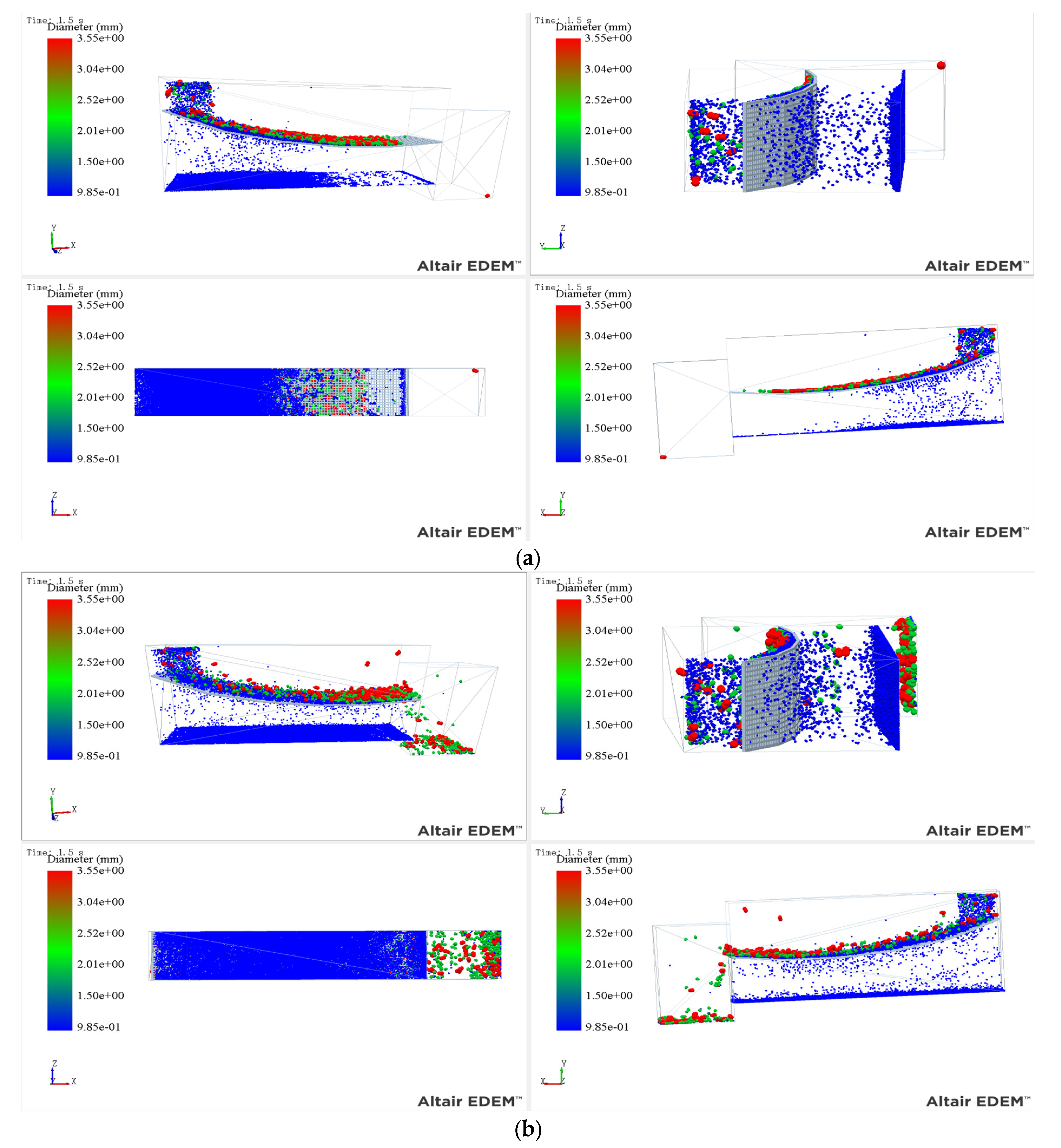
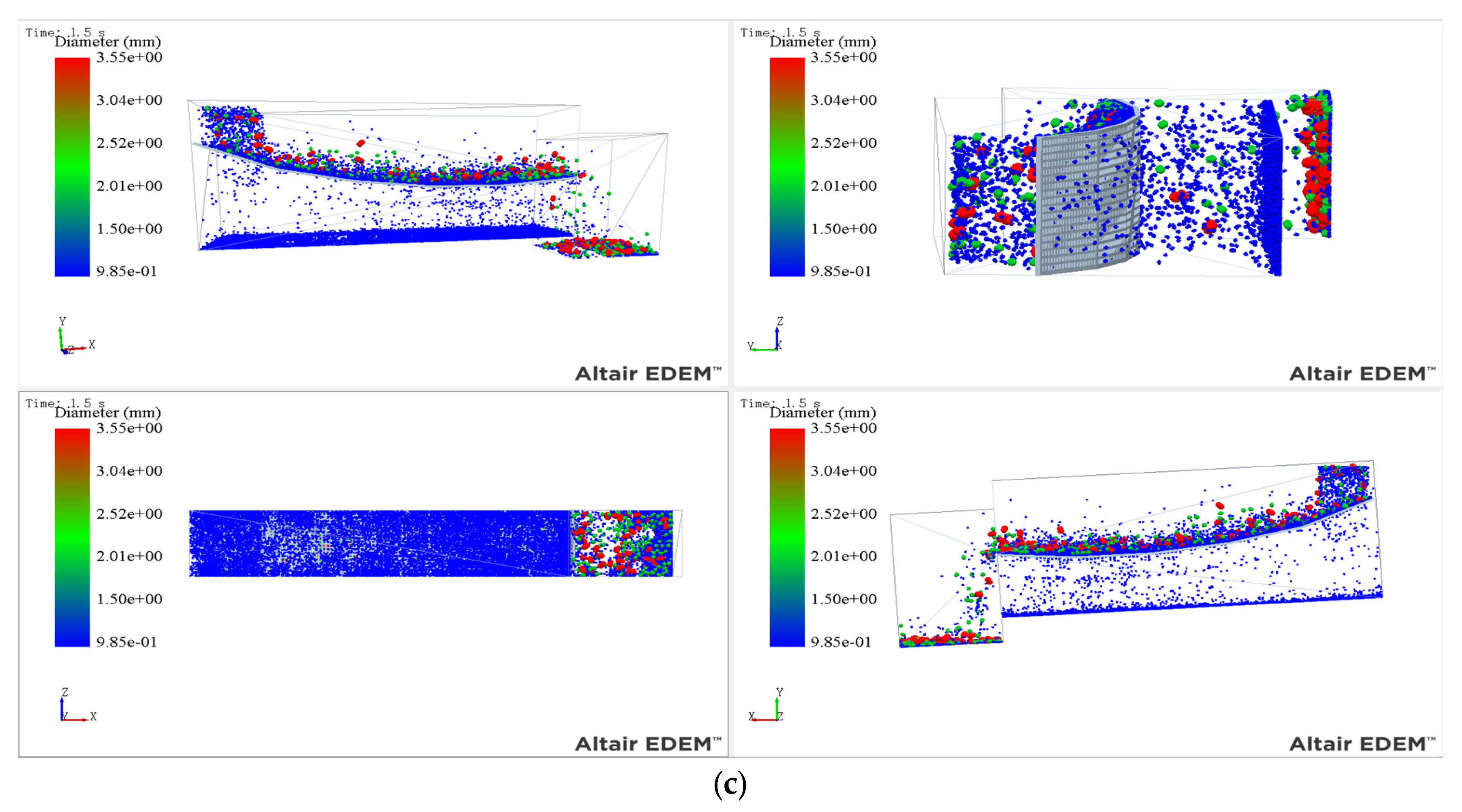
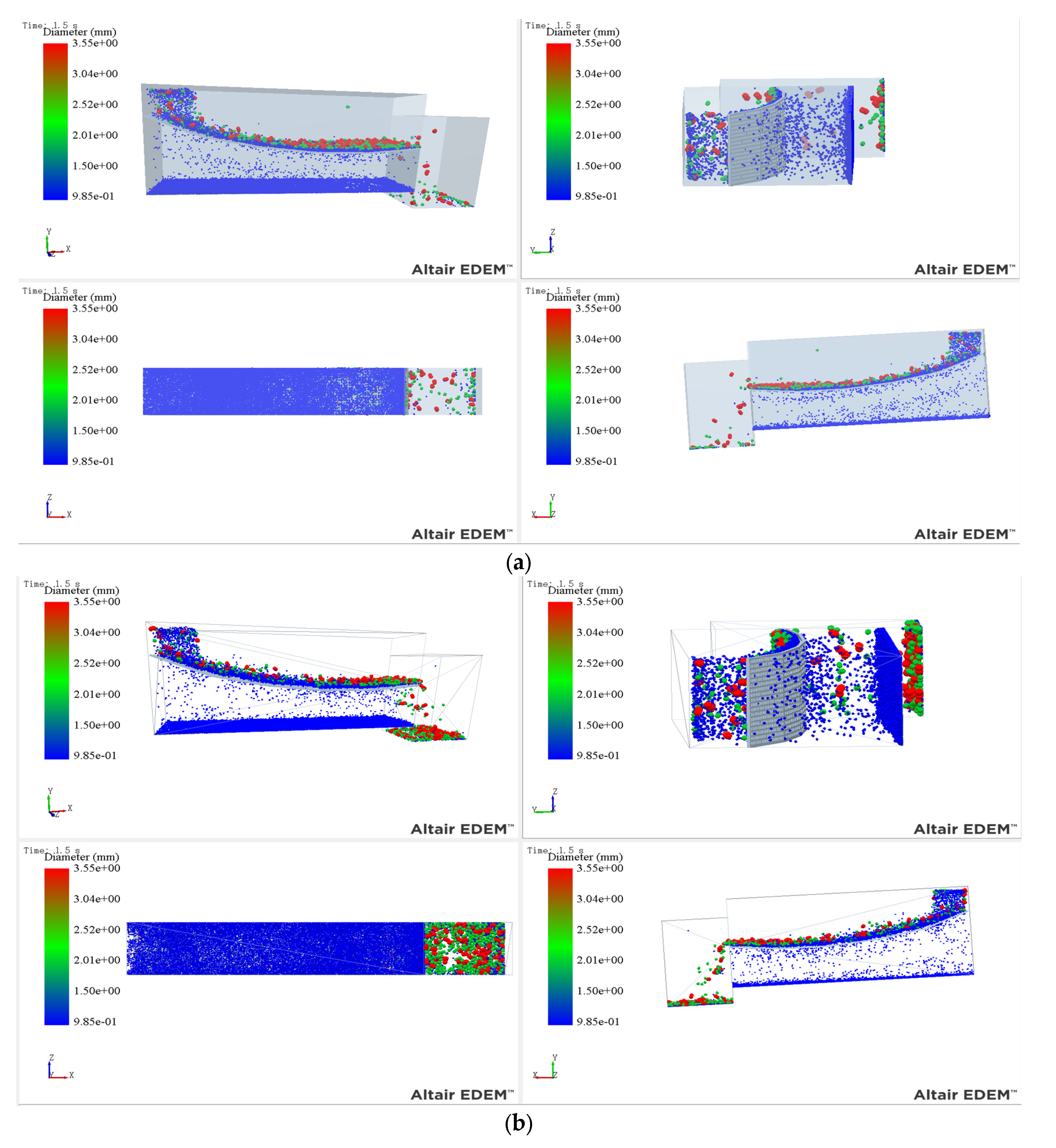
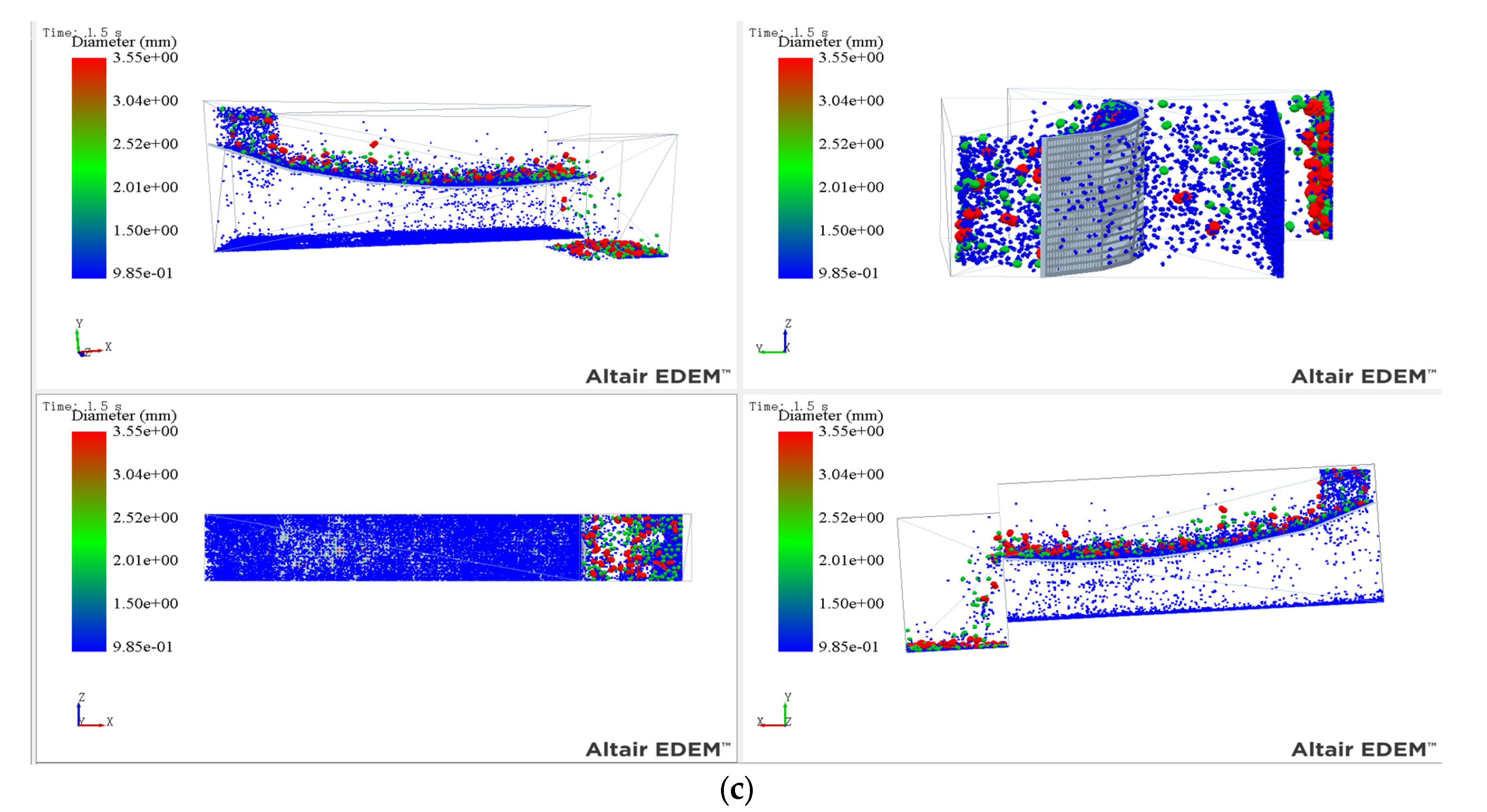
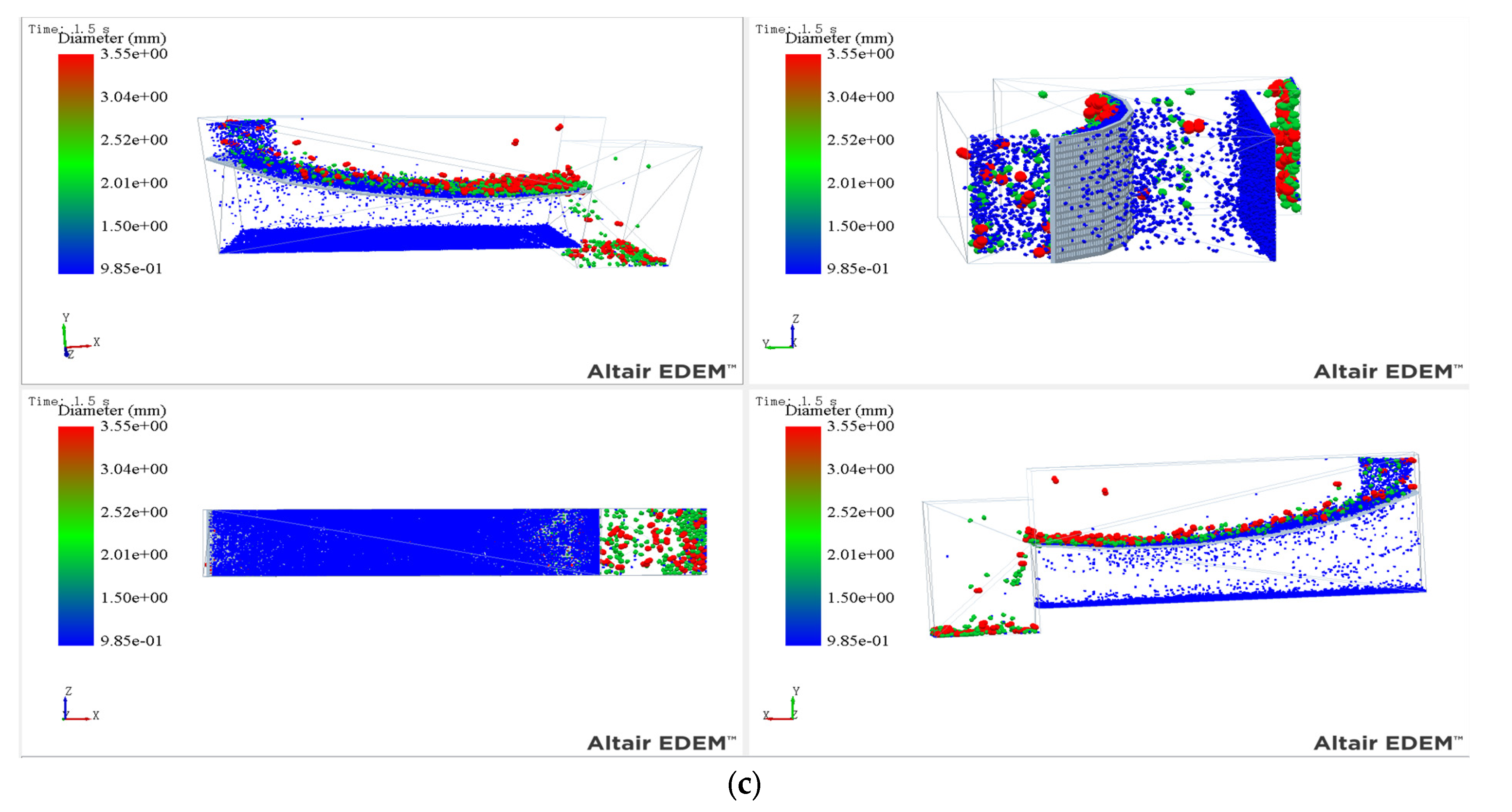
Through the modeling and simulation analysis of the multi-parameter combination of the vibrating screen, the complex parameters were combined and simulated under multiple scenarios. The screening scenario is shown in Figure 3. In order to make the screening scenario under different parameter combinations comparable, the bimodal normal distribution was set to have a 1.5 and 3 mm particle size, the same screening time (time is 1.5 s) was uniformly selected for scene comparison. The numerical simulation revealed that the screening performance of the vibrating screen exhibited diverse features depending on the vibration strength. When the vibration strength was small, the screen performance can be improved significantly by appropriately increasing the vibration strength of the screen, but when the vibration strength was too large, the screen performance showed a downward trend. When other screen parameters were the same (vibration direction angle was 40°, swing frequency was 13, swing Angle was 1.1°, inclination change rate was 0.6), vibration frequency was 10 Hz, vibration amplitude was 1.6 mm, and screening efficiency was 79.84%, as shown in Figure 3a. The loose stratification rate of the material layer was accelerated, the screening probability was higher, and the screening efficiency reached 90.08% when the vibration intensity was properly increased, the vibration frequency was raised to 16 Hz, and the vibration amplitude was 2.2 mm, as shown in Figure 3b. When the vibration intensity continued to increase, the vibration frequency was increased to 22 Hz and the vibration amplitude was 2.8 mm, the material body gained kinetic energy too fast, the stagnation time in the air was prolonged, and the screening efficiency decreased to 81.13%, as shown in Figure 3c. This was due to the fact that as the sieving machine’s vibration intensity increased, the vibration energy provided by the screen surface also sharply increased, causing the material body’s motion acceleration and ejection intensity to increase quickly, the material group’s movement speed to increase, the loosening and layering effects of various particle level material bodies to be improved, the screening rate of the target screening material body to increase, and the screen’s vibration energy to sharply increase. When the sieve surface vibrated too much, the movement of the material body sped up, the spatial expansion range widened, and there was a slight splashing phenomenon. At this point, the coarse-grained material group gained more kinetic energy, and the fine-grained material group lost less kinetic energy.
The vibration direction angle primarily controlled the contact probability between the material group and the screen surface by modifying the material group’s movement direction and contact angle, hence impacting the screen machine’s performance. Figure 4 depicts the screening scene. When the other motion parameters were the same (vibration amplitude was 1.9 mm, vibration frequency was 16 Hz, oscillation frequency was 13 Hz, oscillation angle was 1.1°, and inclination change rate was 0.6), the screening efficiency was 84.84% when the vibration direction angle was 20°, as shown in Figure 4a. When the appropriate lifting direction Angle was 40°, the optimal performance of the screen machine was 90.38%, as shown in Figure 4b. When the direction angle continued to increase to 60°, the material group leap intensified, the space stagnation time was too long, and the screening efficiency decreased to 85.31%, as shown in Figure 4c.
The swing strength of the screening machine is mainly adjusted by the swing frequency and swing angle of the screening machine to change the flow capacity of the screening fabric group, make it evenly distributed and prevent the accumulation of material layers. The screening scene is shown in Figure 5. When other screen parameters were the same (vibration direction angle was 40°, vibration frequency was 13 Hz, vibration amplitude was 1.9 mm, inclination change rate was 0.6), swing frequency was 7 Hz, swing angle was 0.5°, the screening efficiency was 85.12%, the screening scene is shown in Figure 5a. Continued to increase the swing intensity, increase the swing frequency to 13 Hz, swing angle was 0.9°, the screening efficiency increased to 90.38%, the screening scene is shown in Figure 5b. When the swing intensity continued to increase to the dynamic frequency was 19 Hz and the swing angle was 1.3°, the screening machine’s performance began to deteriorate, and the screening efficiency was 84.25%. The screening scene is shown in Figure 5c.
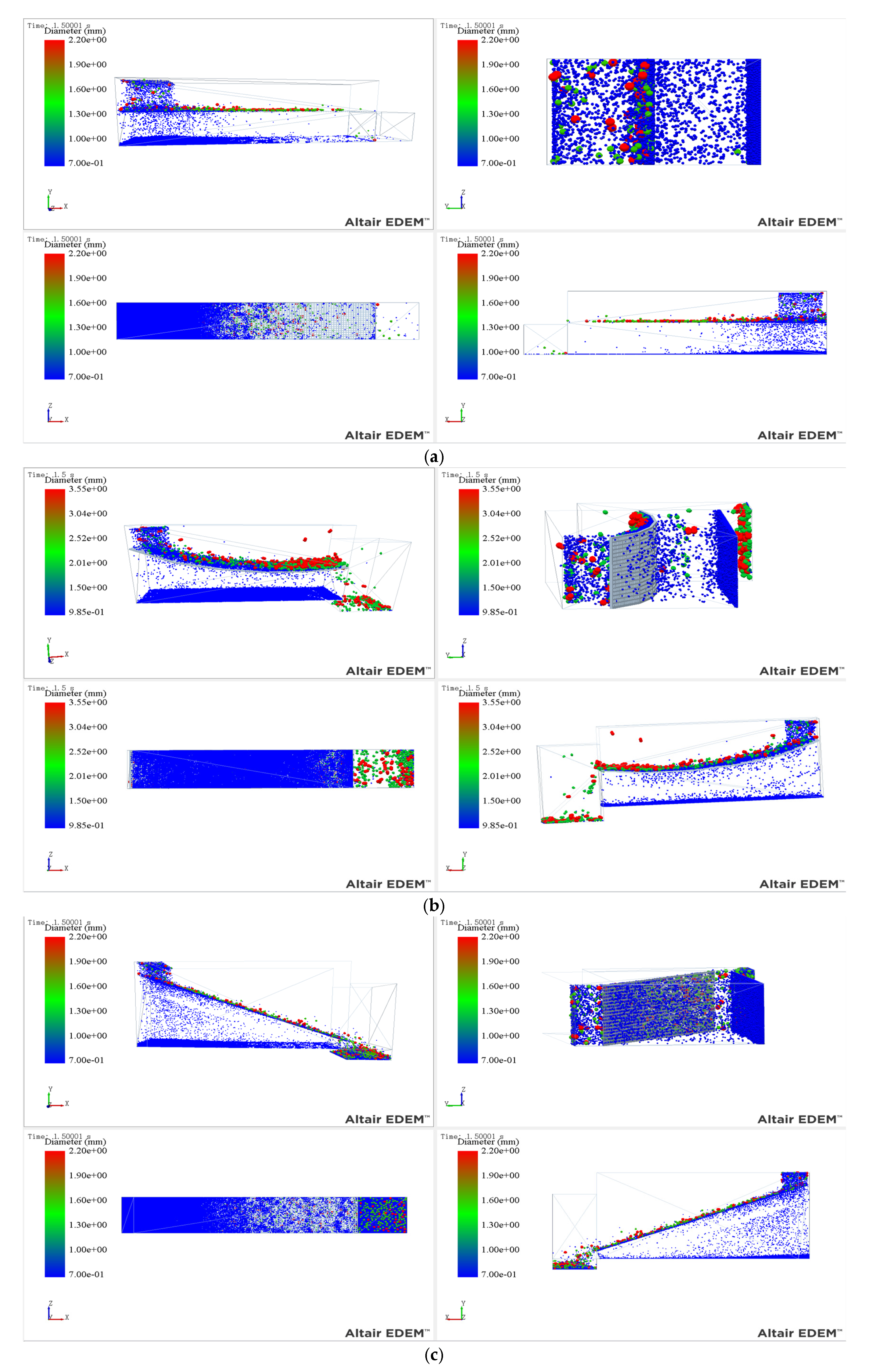
The rate of change of the screen surface inclination angle is directly connected to the material group’s loose movement behavior. Different screen surface design forms have a significant impact on the screening outcomes of the material group in the same feeding scenario [16], and the screening scene was depicted in Figure 6. When the screen surface was flat, the spreading rate of the material group was slow, which made stacking on the screen surface easier. Because coarse-grade material covered the screen surface, fine-grade material cannot fully contact the screen surface, and the likelihood of contacting the screen was considerably decreased. Figure 6a depicted the screening scene, which resulted not only in a reduction in the screening efficiency of the material group but also in a poor usage efficiency of the screen surface when compared to the multi-inclination screen surface. The screening behavior was basically in the first half, and the processing capacity also declined rapidly. However, after the screen surface shape was adjusted for a single and large angle, its processing capacity increased significantly and the average migration rate of the material mass increased rapidly. However, the overspread rate of the material mass in the early stage was too fast, resulting in serious binding of the material mass, and most of the fine-grain material mass was transported before completing the layering effect, resulted in poor screening effect. The screening scene was shown in Figure 6b. The multi-inclination screen surface extended from several stages with different inclination angles, and the material mass group contacted the screen surface to obtain a larger inclination angle, which was convenient for rapid spreading in a short time. The inclination trend decreased with the overall movement of the material mass group, increasing the contact time between the material mass group and the screen surface and substantially improving screening efficiency. Figure 6c depicts the screening scene.

4. BP Neural Network Model Establishment

The BP neural network is a type of computational network that may self-evolve and replicates the thinking process of the human brain [17]. It is now commonly utilized in forecasting the direction of complicated multi-factor nonlinear mapping outcomes, and it is an efficient way for predicting and improving vibrating screen performance under various parameter combinations. As the learning and training model of the BP neural network in this article, a huge amount of screening data were employed. The network’s iterative calculation is carried out continuously, and the sample database and influence weights are constantly improved, so that the network can predict and optimize screening machine performance under different parameters efficiently and accurately.

4.1. Backpropagation Neural Network (BPNN)

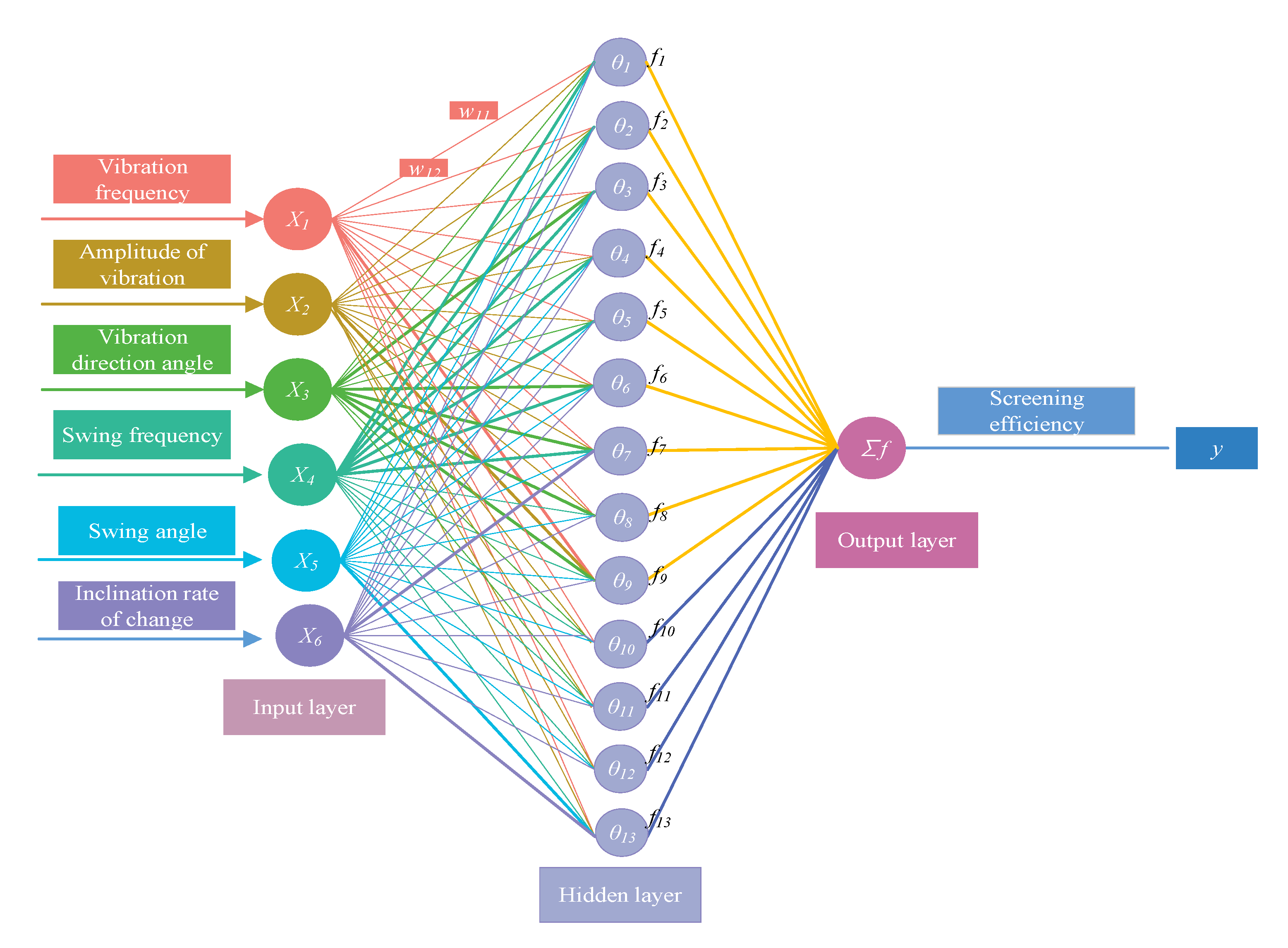
The backpropagation neural network (BPNN) is a multi-level feedback error propagation network that has the characteristics of spontaneous evolution and self-development. Its main structure is composed of an input layer, a hidden layer, and an output layer. The former is mainly responsible for the input of independent variables. The next latter is responsible for analyzing and extracting the independent variables’ characteristics. The latter is the desired prediction results for different parameter combinations. When predicting the performance of vibrating screen at multi-parameter complex level, it is very important to determine the different input layers, hidden layers and computing nodes for the accuracy of prediction data. Because the amplitude, vibration frequency, vibration direction angle, swing frequency, swing angle, and the change rate of screen surface inclination have the greatest influence on screen machine performance, these six parameters were used as the network structure’s input layer. However, due to the obvious differences in their units and values, they need to be normalized in the hidden layer to make their parameters are between (0 and 1), which is convenient for the continuous updating, learning, and evolution of the network [18].
As an important structure for feature extraction and transformation of input variables, the hidden layer can not only display the change trend of a single parameter, but also realize the influence of complex nonlinear mapping relationships. Its structural forms are diverse, not only can be composed of single-layer structures but also can be displayed by multi-layer complex structures. In this paper, the Sigmoid model was used as a tool to extract complex features of hidden layer, so as to accurately extract and transmit the feature range of independent variables to the output layer structure [19]. After a large number of experiments, it was found that the screen machine parameter combination optimization can be completed by using a hidden layer structure, and the number of nodes in the hidden layer was calculated as 13 by empirical Equation (3).
n = 2x + 1
where n is the number of nodes in the hidden layer of the neural network and x is the number of input layer nodes.
This paper built the BP neural network model based on the feedforwardent function. Based on multiple screening data training and learning results, the weight connections between each layer of the network were accurately connected to determine the influence range of each parameter in the network. When the learning rate was 0.01, the number of cycles was 1000, and the accuracy of the network was 1 × 10⁻⁵, a three-layer neural network prediction model with six inputs, one hidden layer with 13 nodes, and one output can be constructed with high accuracy. The model is shown in Figure 7.
Where, the input layer can be represented by a vector X, which means X = (x1, x2, x3, x4, x5, x6). The weighting coefficient of the hidden layer can be represented by the vector W, that is, W = (w1, w2,...... wi, …… w13)T, after weighted calculation of input layer data, the input weighted sum was calculated according to Equation (4), θ is Sigmoid type activation function, f is a mapping function, which maps the data of the input layer to the output layer through some mapping relationship. The output layer vector is Y = (y1) [20], and its calculation Equation (5) is shown as follows.
Enter   the   weighted   sum :   n = j = 1 n w i j x j θ i
Output : y i = f ( j = 1 n w i j x j θ i )

4.2. Integrated Learning and Prediction of Models

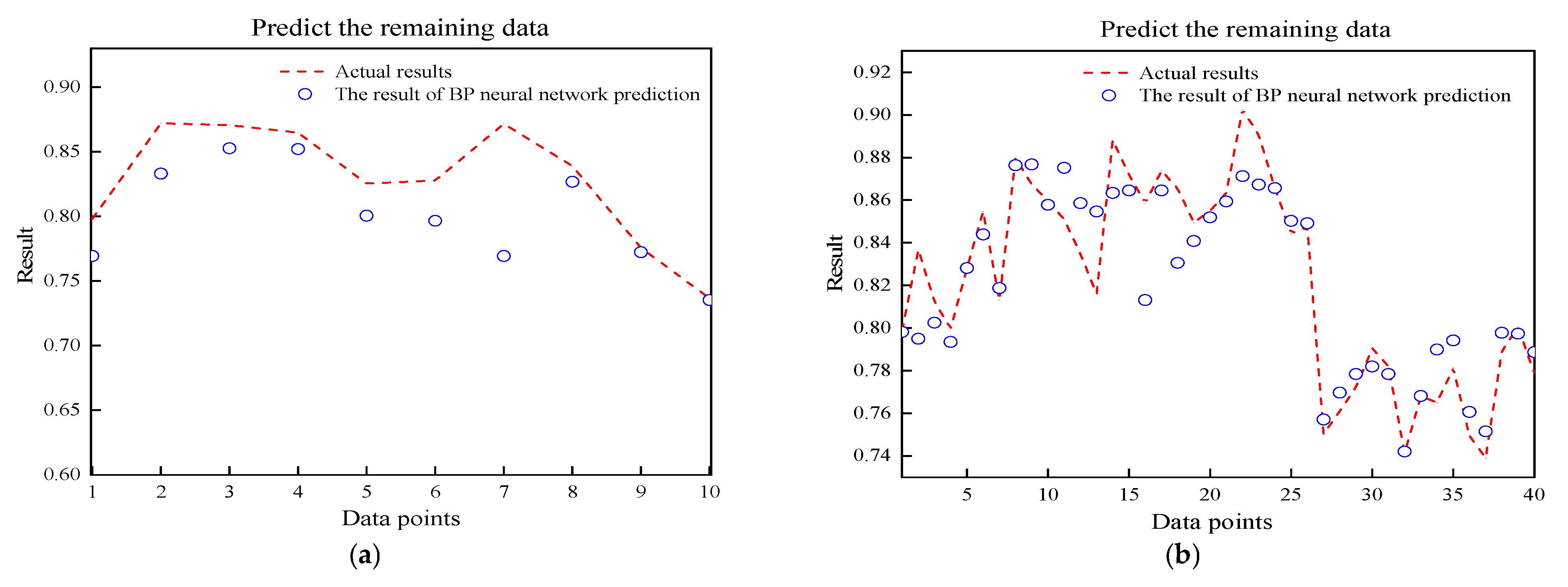
The orthogonal test simulation of six parameters was carried out with discrete element software EDEM as the carrier. The screening efficiency of the first 40 groups of screening machines was obtained, which was the training set. The screening efficiency of the last 10 groups of data needed to be tested by the model, which was the test set. In this article, data from groups 1 to 50 were used as training samples and were imported into the BP neural network to develop the algorithm’s original model, as shown in Figure 8.
The structure responsible for distinct functions was automatically separated into three portions while the neural network was operating. In this article, for example, the vibration frequency, amplitude, vibration direction angle, inclination rate, swing frequency, and swing angle were chosen as the input layer because they have the largest influence on the operation of the screen machine. The part extracted from the important features of the factors was taken as the hidden layer. Finally, the screening efficiency, which represent the performance of the screening machine, was taken as the output layer, and the initial model was constantly trained and tested. From Figure 8, it can be seen that the predicted curve and the true value curve had a similar increase or decrease trend, proving that the trained model has a certain accuracy in predicting the parameters of the screening machine. The nonlinear mapping relationship under the complex parameter changes was reflected from the fluctuation of the target parameters of the screen machine, which proved the practicability of Ensemble learning modeling for the prediction of screen machine parameter changes.

4.3. Analysis of Model Prediction Results

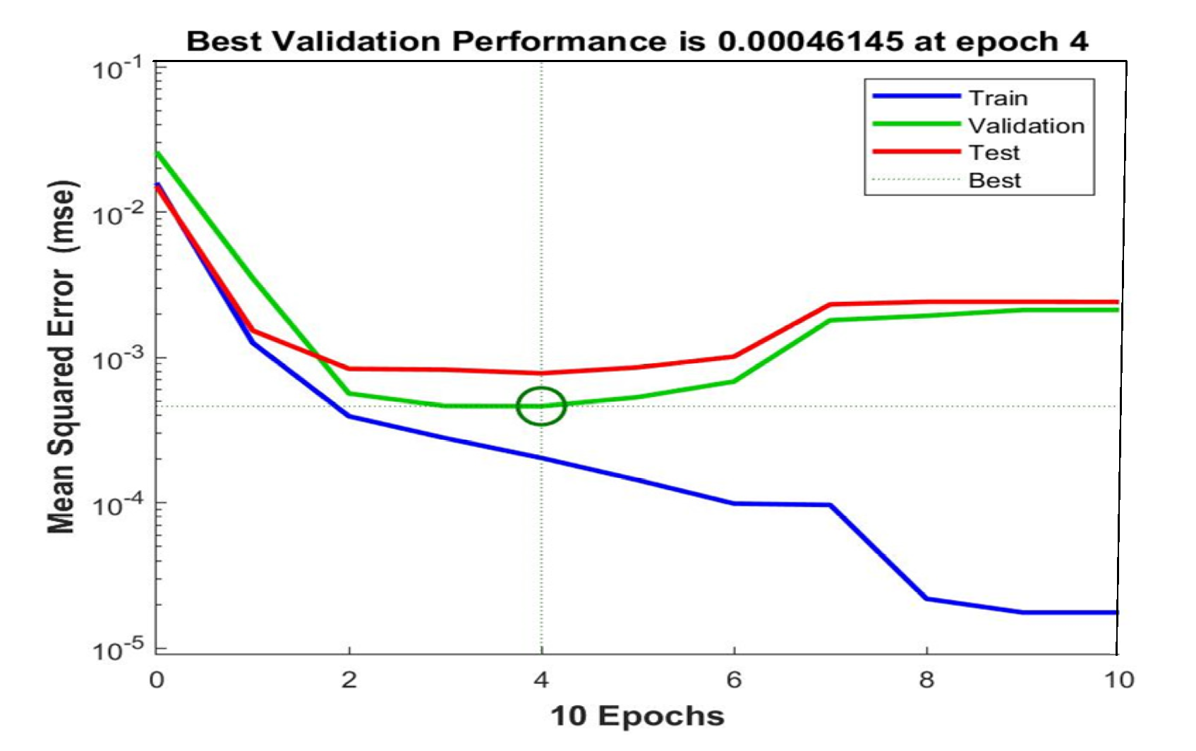
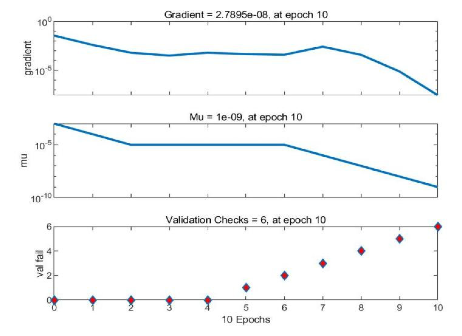
When a BP neural network is activated, it randomly groups the collected data into three groups. These three groups are training, verification, and prediction. Each of these will generate a mean square error (MSE). Figure 9 illustrated the change rule for mean square error with network iteration times. The minimal mean square error of the data from the training, verification, and prediction groups first appeared when the screening effect was predicted for the fourth time, as shown in Figure 10, and it continued to exist until the error converged and the network training was stopped. In this experiment, the mean square error convergence was attained after the tenth attempt, and the BP neural network training was terminated.
The accuracy of the created network model was quite steady after 10 rounds, as evidenced by the BP neural network training state diagram (Figure 10). After obtaining the best model performance, the weights of the 10th network training results were eventually used as the final response proportion to be modeled by the neural network so as to forecast the output layer based on the matching input layer data.
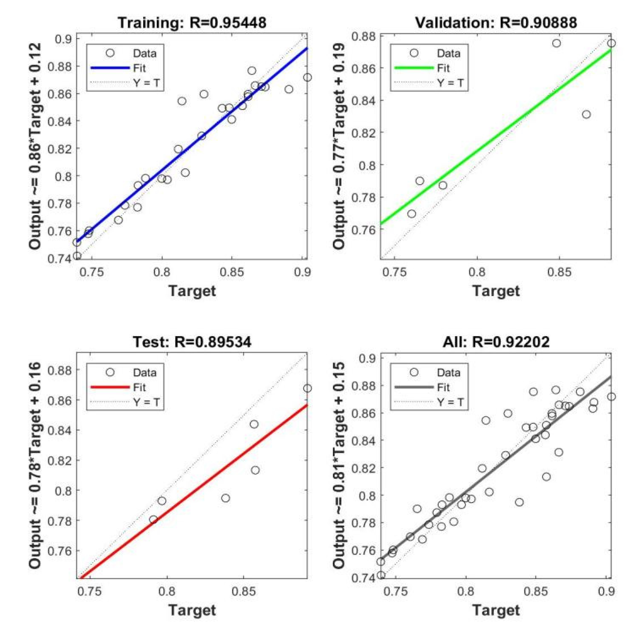
Figure 11 displayed the regression analysis diagram for the BP neural network training. Figure 11 shows that the training sample, test sample, and overall prediction result all had regression coefficient R values of 0.9545, 0.9089, 0.8953, and 0.9220, respectively. The model was better established the closer the R value was to 1. The four R values achieved in this experiment were all very near to one, demonstrating the superiority of the established model and its increased prediction accuracy.

4.4. Analysis of Impact Weights

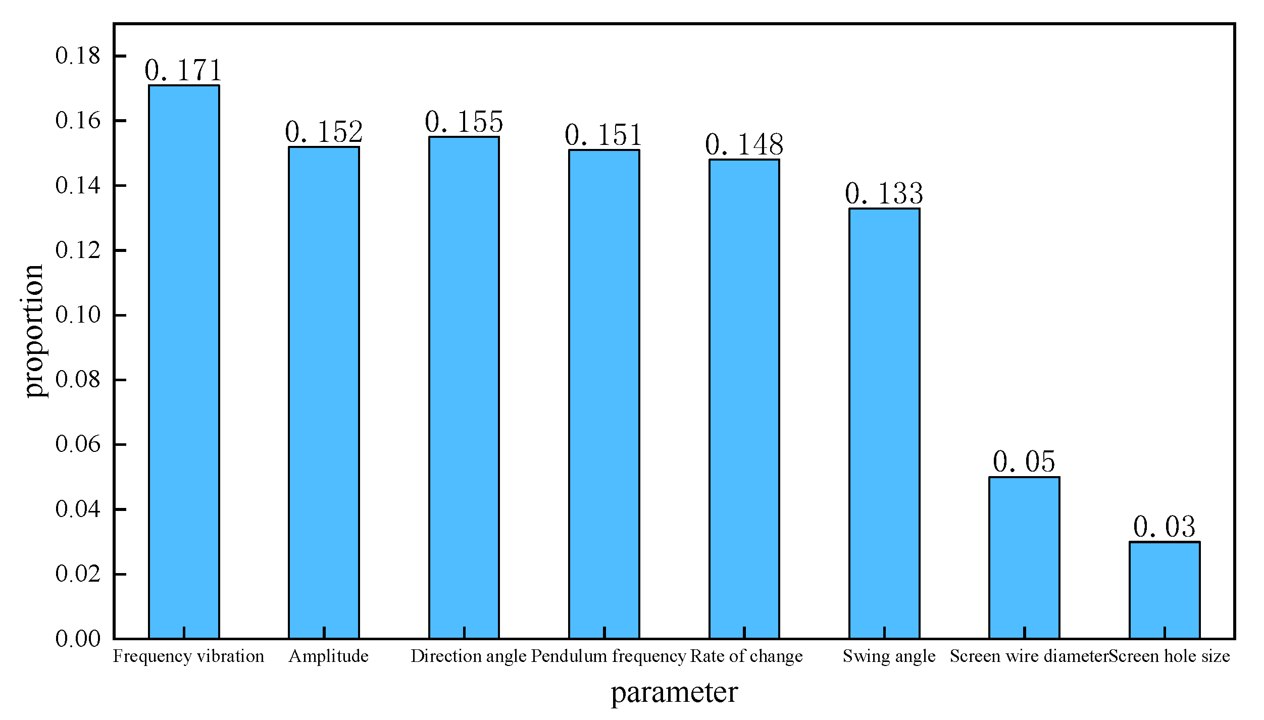
A number of factors, such as vibration amplitude, vibration direction angle, vibration frequency, change rate of screen surface inclination angle, screen wire diameter, swing frequency, swing angle, etc., affect a screening machine’s performance. Although different parameters affect how well the screening machine performs, the weight of that impact varies. When processing the screening score data, it is crucial to be clear about the relative contributions of the various parameters to the screening results. Therefore, in this paper, the weight analysis of the influence of factors on each parameter was carried out in the way of ensemble learning to clarify the key factors of this experiments. Figure 12 displayed the weight of the impact of screen motion settings on screening effectiveness.
According to Figure 12, the vibration frequency, amplitude, vibration direction angle, inclination rate of change, swing frequency, and swing angle have the greatest effects on the performance of the screen machine. These factors’ weights were 0.171, 0.152, 0.155, 0.151, 0.148, 0.133, 0.050, and 0.030, respectively. As a result, the parameters of the secondary sixth sieve machine are mostly used as the independent variable in this article’s modeling and optimization analysis, and corresponding parameter interaction combination analysis is performed based on its parameter weight size.

5. Optimization of BP Neural Network by PSO Algorithm

5.1. Particle Swarm Optimization

The particle swarm optimization (PSO) algorithm is often used in group optimization calculation, and it is widely used in various complex networks for its simple operation, accurate convergence, fast convergence, and optimization adjustment. Its main operating principle was to initialize the particle swarm in the feasible solution space, and carried out spatial iterative calculation to find the optimal interval of particles with complex interactions among particle swarm, so that different particles have the potential of extreme optimal solutions. Finally, the particle swarm characteristics were characterized with the position, velocity, and fitness value as the three most important indicators. The BP neural network realized self-learning mainly by refining the weight and threshold, but it may be affected by the local minimum during local correction, which will cause errors to the overall network structure. It is mentioned to try to reduce this type of mistake and speed up network response time. The structure of the BP neural network is optimized using particle swarm optimization (PSO) [21], and a model for the PSO-BP neural network is developed. Setting BP neural network settings is not necessary in this method. Instead, by employing its superior global search capabilities to find the most appropriate connection weights and thresholds in various structural layers of the neural network algorithm while continuously updating the position and speed of people in the particle swarm.
The threshold and specific gravity of the hidden layer in the BP neural network were optimized using particle swarm optimization to increase unpredictability and enhance the hidden layer’s capacity for global search. The following is the precise operation sequence.
(1) The obtained simulation screen scores were normalized according to the set, and the influence ability was characterized by the unified value. With input layer node 6, hidden layer node 13, and output layer node 1, a neural network model was created, and the weight was found to be 6 × 13 + 13 × 1 = 91. The cutoff value is 13 + 1 = 14.
(2) Define the PSO algorithm’s boundary parameters: set the particle swarm size N, position boundary [Xmin, Xmax], velocity critical value [Vmin, Vmax], inertia weight w, number of iterations k, acceleration learning factors c1, c2, etc. [22], and initialize the velocity Vi and position Xi. The PSO algorithm has a variety of parameters, which need to be combined with experience and defined formulas to obtain. The particle dimension is calculated by Equation (6).
D = (x + 1) n + (n + 1) p
where x is the number of nodes in the input layer; n is the number of hidden layer nodes; p is the number of output layer nodes.
The particle dimension D = 105 in the PSO-BP neural network model can be obtained by the formula, and other parameters were set to N = 20, Vmin = −3, Vmax = 3, w = 0.9, k = 200, c1 = 2.7, c2 = 1.3.
(3) The mean squared error was determined using the actual input and output sample values, as well as the anticipated values of the model, and was utilized as the fitness function of the PSO algorithm. Using Equation (7), the fitness values of various particles were calculated, and the population’s individual optimum solution Pbest and global ideal solution Gbest were recorded.
The fitness values are:
f i t n e s s = 1 a i = 1 a j = 1 p ( Y i j y i j )  
where a is the sample size; p is the number of output neurons; Y i j is the j-th output expected value of the i-th sample; y i j is the actual value of the jth output of the i-th sample.
(4) Update the particle’s velocity and location using Equations (8) and (9).
The velocity of each swarm was modified throughout the swarm iteration to [21]:
V i d k + 1 = w V i d k + c 1 r 1 P i d k X i d k + c 2 r 2 P g d k X g d k
where Vid is the d-dimensional velocity of the i-th sample; Pid is the d-dimensional individual extreme of the i-th sample; Pgd is the d-dimension of the global optimal solution; k is the number of iterations; c1 and c2 are acceleration learning factors; w is the inertia weight; r1 = r2 represents a random number in the range [0, 1].
During the swarm iteration, the position of each particle swarm was updated to [23]:
X i d k + 1 = X i d k + V i d k + 1
(5) Iterative operation, individual extremum, and group extremum between different particles were found. When the fitness value fi of particle i was compared to the individual optimal value Pbest, if its value was less than Pbest, it was replaced as individual optimal; when the fitness value fi was compared to the global extreme value Gbest, if its value was less than Gbest, it was replaced as global optimal [24].
(6) The iterative calculation of the algorithm is completed, and the overall optimal particle characteristics are mapped to the neural network to complete the repair definition of its weights and thresholds.
(7) The collected sample data will be tested for network response, and the results of unknown parameter combination data will be predicted.

5.2. Model Performance Evaluation

When the network model was finished, it is critical to examine the accuracy and response efficiency of the present model. As a result, the five evaluation indices of root mean square error (RMSE), mean square relative error (MSRE), mean absolute error (MAE), mean absolute relative error (MARE), and determination coefficient R2 were used in this paper to evaluate the performance of the PSO-BP neural network model. The greater the inaccuracy, the greater the value, and the poorer the model’s predictions. As a result, the RMSE, MSRE, MAE, and MARE values were low, and the greater the R2 value, the better the predictive performance of the model.

5.3. Analysis of Prediction Results

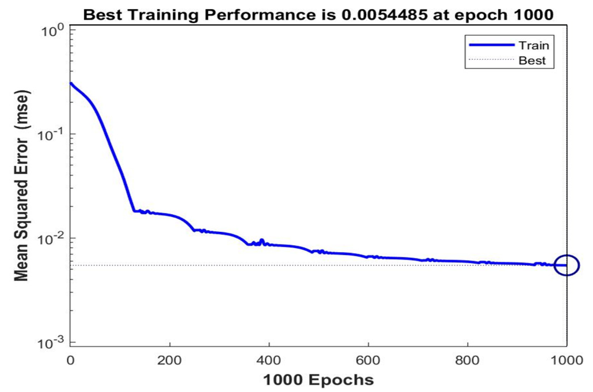
Figure 13 depicted the network’s training status, which showed that the network model achieves the best performance after 1000 training iterations, and after achieving the best performance, the RMSE of the network was 0.0054, and the neural network model finally takes the weight generated by the 1000th network training as the final weight, in order to predict the output layer based on the corresponding input layer data.
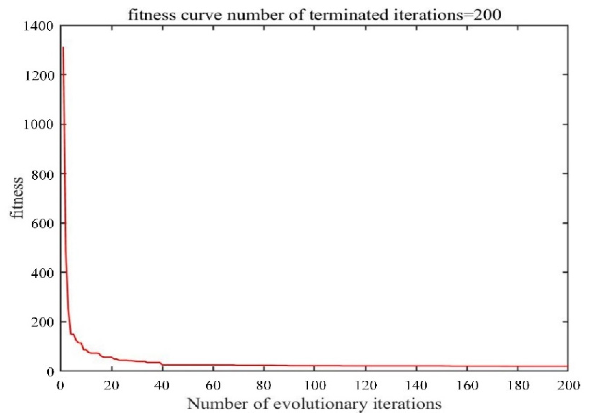
When the number of iterations increased sequentially, the particle fitness value dropped. When the number of iterations hit 200, the particle fitness value settled into a limited and stable zone, as illustrated in Figure 14. The particle’s performance improved when its fitness value decreased.
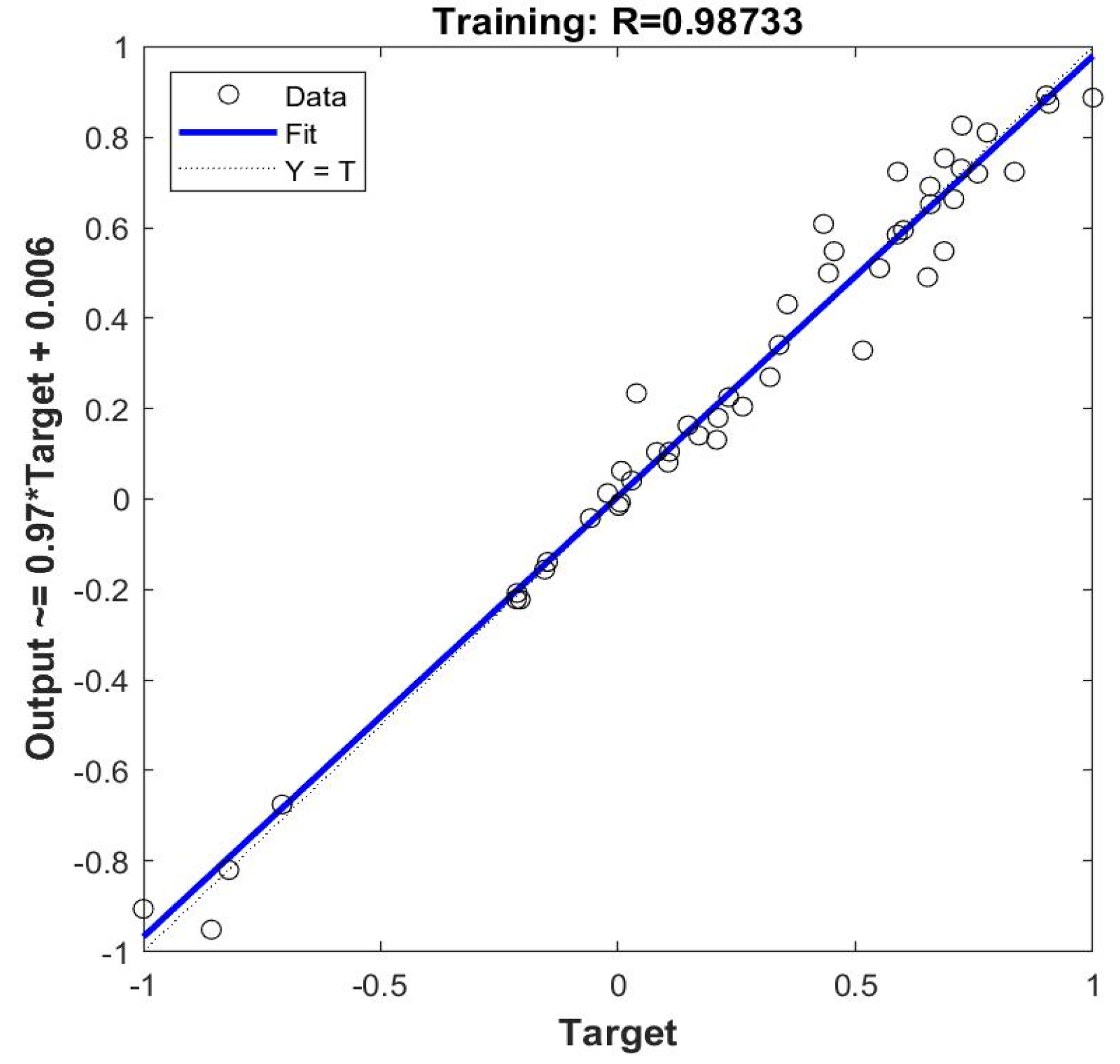
Figure 15 depicted the regression analysis graph trained by the PSO-BP neural network. The network’s prediction result was 0.9873, which was closer to 1 than the regression coefficient R value of the BP neural network. Additionally, the prediction regression line is typically distributed in the center of the data point and fits the data more closely, demonstrating that the created model was more accurate at making predictions than the BP neural network alone.
Figure 16 showed a comparison of the prediction model accuracy between the actual value and the predicted value of the sample using BP neural network and PSO-BP neural network when the model was used to forecast the instantaneous screening efficiency under different parameter combinations. Figure 16 showed that when the PSO-BP neural network predicted sieving efficiency, the relative error of 33 of the 50 training samples was positive, indicating that the predicted value was greater than the true value, and the relative error of 16 samples was negative, indicating that the predicted value was less than the true value, and the RMSE, MSRE, MAE, and MARE were 0.0184, 0.0132, 0.0102, 0.0050, indicating that the model error was small.
To validate the data model’s accuracy, 50 sets of data were chosen and the errors of the PSO-BP neural network and BP network model data were compared. It was discovered that the PSO-BP neural network had lower error and higher network accuracy, implying that the predicted screening efficiency of the obtained model was more realistic.
Table 4 showed that the RMSE, MSRE, MAE, and MARE predicted by BP neural networks were 0.0795, 0.0416, 0.0482, and 0.0230, respectively, while the prediction results of PSO-BP neural networks were 0.0184, 0.0132, 0.0102, and 0.0050, respectively. These results demonstrate that PSO-BP neural networks were more accurate than BP neural network models in terms of RMSE, MSRE, MAE, and MARE predictions. The prediction accuracy of the PSO-BP neural network was greater than that predicted by the BP neural network since the R2 was 0.9748 higher than the 0.9110 of the BP neural network model.

6. Conclusions

(1) Based on the results of the field screening test, this paper maintained the prototype’s streamlined screening feature parts, recreated the realistic and complex parameter scenes of the actual screening with the idealized model machine, and creatively suggested to change the gradient of the screen surface inclination. It also investigated the temporal and spatial distribution law of particle groups using the three-dimensional discrete element method and revealed the screening mechanism of complex particles.
(2) Obtain screening test data in multiple scenarios based on simulation experiments, and import the obtained 50 sets of test data into a BP neural network with strong training and learning capabilities to achieve sample data learning and prediction, as well as the impact weight proportion of multiple different screening machine parameters on screening efficiency. After evaluating the data with the created BP neural network model, it was determined that the minimum mean square error occurred in the fourth iteration, and the error converged in the tenth iteration, when neural network training was terminated.
(3) The PSO method was suggested for optimization in order to further enhance the generalization capability of the BP neural network model for forecasting and improving screening test parameters. The screening machine data model’s ideal solution was looked for using the modified PSO-BP neural network technique. The following parameter combinations were found to be the most effective: 1.93 mm amplitude, 16.28 Hz vibration frequency, 40.38° vibration direction angle, 1.08° swing angle, 12.1 Hz swing frequency, and 0.6° inclination rate. The PSO-BP neural network and the BP network model data were compared in terms of error in order to confirm the correctness of the data model. The PSO-BP neural network’s various faults were discovered to be quite minimal, leading to a model that more correctly predicted screening efficiency.

Author Contributions

Conceptualization, J.Z. and Y.W. (Yan Wang); investigation, J.Z., F.N., Y.W. (Yan Wang), H.Z. and S.L.; methodology, H.Z., F.N. and Y.W. (Yanpeng Wang); formal analysis, F.N., J.Z., Y.W. (Yan Wang) and S.L.; data curation, Y.W. (Yan Wang), F.N., H.Z., J.Z. and Y.W. (Yanpeng Wang); writing—original draft preparation, Y.W. (Yan Wang), J.Z., H.Z. and S.L.; writing—review and editing, J.Z., Y.W. (Yan Wang), H.Z. and Y.W. (Yanpeng Wang); project administration, F.N. and J.Z.; funding acquisition, F.N. All authors have read and agreed to the published version of the manuscript.

Funding

This work was supported by Central Guiding Local Science and Technology Development Fund Projects (226Z4104G); Scientific and Technological Research Projects in Colleges and Universities in Hebei Province (ZD2022128); Tangshan Science and Technology Plan Project (22130226H).

Data Availability Statement

Data available on request due to restrictions privacy. The data provided in this study can be obtained at the request of the corresponding author. As the data needs further research, the data is currently not publicly available.

Acknowledgments

The researchers are grateful for the support of EDEM and MATLAB software for the research.

Conflicts of Interest

The authors declare no conflict of interest.

Abbreviations

BPBackpropagation
MAEMean Absolute Error
MAREMean Absolute Relative Error
MSREMean Square Relative Error
PSOParticle Swarm Optimization
PSO-BPParticle Swarm Optimization-Backpropagation
RMSERoot Mean Square Error

References

  1. Shen, G.; Chen, Z.; Wu, X.; Li, Z.; Tong, X. Stepwise shape optimization of the surface of a vibrating screen. Particuology 2021, 58, 26–34. [Google Scholar] [CrossRef]
  2. Yu, C.; Lin, D.; Wang, X.; Pu, K.; Wang, Z.; Zhao, G.; Geng, R.; Gong, S. DEM simulation of particle flow and separation in a vibrating flip-flow screen. Particuology 2023, 73, 113–127. [Google Scholar] [CrossRef]
  3. Li, Y.; Fan, H.; Xu, Y.; Cui, T.; Su, Y.; Qiao, M.; Han, S.; Qian, J.; Zheng, Z. CFD-DEM investigation of particle dispersion degree on a novel vibrating screen. Powder Technol. 2022, 404, 117497. [Google Scholar] [CrossRef]
  4. Chen, Z.; Li, Z.; Xia, H.; Tong, X. Performance optimization of the elliptically vibrating screen with a hybrid MACO-GBDT algorithm. Particuology 2021, 56, 193–206. [Google Scholar] [CrossRef]
  5. Wang, G.; Chen, S.; Hu, G.; Pang, D.; Wang, Z. Detection algorithm of abnormal flow state fluid on closed vibrating screen based on improved YOLOv5. Eng. Appl. Artif. Intell. 2023, 123, 106272. [Google Scholar] [CrossRef]
  6. Ahad, A.H.; Caner, O.E.; Levent, E.S. Discrete element modelling of vibrating screens. Miner. Eng. 2018, 121, 107–121. [Google Scholar]
  7. Lin, D.; Ji, J.C.; Wang, X.; Wang, X.; Wang, Y.; Xu, N.; Ni, Q.; Zhao, G.; Feng, K. A rigid-flexible coupled dynamic model of a flip-flow vibrating screen considering the effects of processed materials. Powder Technol. 2023, 427, 118753. [Google Scholar] [CrossRef]
  8. Zhao, G.; Pu, K.; Xu, N.; Gong, S.; Wang, X. Simulation of particles motion on a double vibrating flip-flow screen surface based on FEM and DEM coupling. Powder Technol. 2023, 421, 118422. [Google Scholar] [CrossRef]
  9. Jiang, H.; Duan, C.; Wu, J.; Zhao, Y.; Liu, C.; Luo, Z.; Dong, L.; Zhang, B.; Wang, Z.; Zhang, C.; et al. Kinematics characteristics of the vibrating screen with rigid-flexible screen rod and the behavior of moist coal particles during the dry deep screening process. Powder Technol. 2017, 319, 92–101. [Google Scholar] [CrossRef]
  10. Xiao, J.; Tong, X. Particle stratification and penetration of a linear vibrating screen by the discrete element method. Int. J. Min. Sci. Technol. 2012, 22, 357–362. [Google Scholar] [CrossRef]
  11. Xia, X.; Gou, L.; Zhang, Z.; Wang, L.; Guo, Y.; Jing, W. Collaborative optimization of linear vibrating screen screening efficiency and dynamic response stability based on coupled DEM-MBK simulation. Particuology 2023, 78, 49–61. [Google Scholar] [CrossRef]
  12. Zhao, Z.; Jin, M.; Qin, F.; Simon, X. Yang. A novel neural network approach to modeling particles distribution on vibrating screen. Powder Technol. 2021, 382, 254–261. [Google Scholar] [CrossRef]
  13. Xu, Z.; Li, Y.; Wan, L.; Ma, X.; Song, J.; Huang, J. Optimising the design of ball racks to improve the sorting efficiency of vibrating screen seed cleaners using discrete element method modelling and experiment. Biosyst. Eng. 2023, 225, 99–117. [Google Scholar] [CrossRef]
  14. Liu, H.; Jia, J.; Liu, N.; Hu, X.; Zhou, X. Effect of material feed rate on sieving performance of vibrating screen for batch mixing equipment. Powder Technol. 2018, 338, 898–904. [Google Scholar] [CrossRef]
  15. Li, Z.; Si, Q.; Jia, P.; Xiao, G.; Tong, X. Research on particle swarm screening mechanism and performance optimization based on simulated lunar microgravity. Adv. Space Res. 2023, 063, 0273–1177. [Google Scholar] [CrossRef]
  16. Barbosa, V.P.; Menezes, A.L.; Gedraite, R.; Ataíde, C.H. Vibration screening: A detailed study using image analysis techniques to characterize the bed behavior in solid–liquid separation. Miner. Eng. 2020, 154, 106383. [Google Scholar] [CrossRef]
  17. Chen, J.; Hsieh, H.; Do, Q. Forecasting Hoabinh Reservoir’s Incoming Flow: An Application of Neural Networks with the Cuckoo Search Algorithm. Information 2014, 5, 570–586. [Google Scholar] [CrossRef] [Green Version]
  18. Dong, S.; Zhou, D.; Zhou, W.; Ding, W.; Gong, J. Research on Network Traffic Identification Based on Improved BP Neural Network. Appl. Math. Inf. Sci. 2013, 7, 389–398. [Google Scholar] [CrossRef]
  19. Ning, Y.; Fuh, J.Y.H.; Wong, Y.; Loh, H.T. An intelligent parameter selection system for the direct metal laser sintering process. Int. J. Prod. Res. 2004, 42, 183–199. [Google Scholar] [CrossRef]
  20. Feng, Z.; Min, X.; Jiang, W.; Song, F.; Li, X. Study on Thermal Error Modeling for CNC Machine Tools Based on the Improved Radial Basis Function Neural Network. Appl. Sci. 2023, 13, 5299. [Google Scholar] [CrossRef]
  21. Silva, T.M.P.; Hameury, C.; Ferrari, G.; Balasubramanian, P.; Franchini, G.; Amabili, M. Particle swarm optimization of a non-collocated MIMO PPF active vibration control of a composite sandwich plate. J. Sound Vib. 2023, 555, 117723. [Google Scholar] [CrossRef]
  22. Lu, Y.; Liang, S.; Ouyang, H.; Li, S.; Wang, G. Hybrid multi-group stochastic cooperative particle swarm optimization algorithm and its application to the photovoltaic parameter identification problem. Energy Rep. 2023, 9, 4654–4681. [Google Scholar] [CrossRef]
  23. Huang, H.; Qin, H.; Hao, Z.; Lim, A. Example-based learning particle swarm optimization for continuous optimization. Inf. Sci. 2011, 182, 125–138. [Google Scholar] [CrossRef]
  24. Fu, X.; Zheng, Q.; Jiang, G.; Roy, K.; Huang, L.; Liu, C.; Li, K.; Chen, H.; Song, X.; Chen, J.; et al. Water quality prediction of copper-molybdenum mining-beneficiation wastewater based on the PSO-SVR model. Front. Environ. Sci. Eng. 2023, 17, 98. [Google Scholar] [CrossRef]
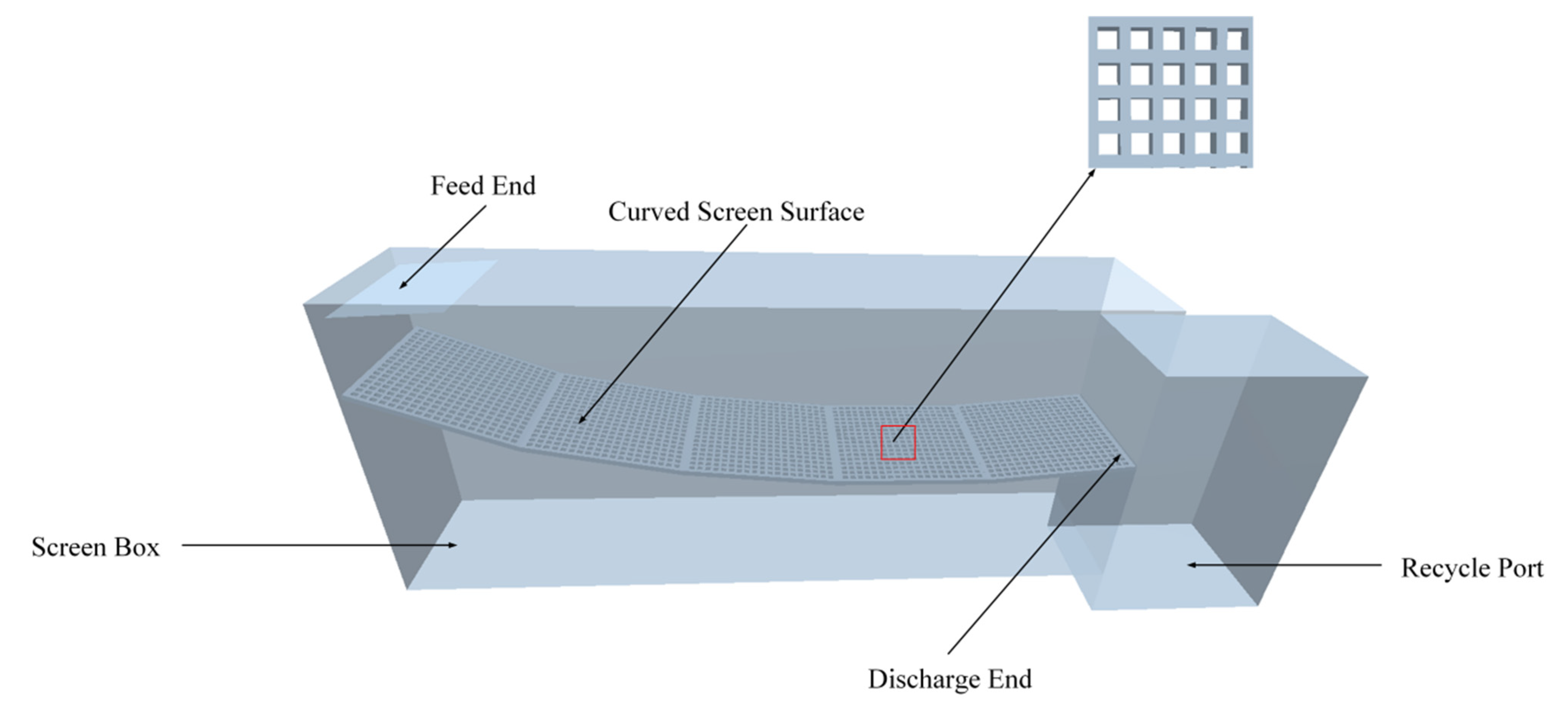
Figure 1. Simplified model of vibrating screen in EDEM software.
Minerals 13 00929 g001
Figure 2. Screening process of simplified model of vibrating screen in EDEM software: (a) t = 0 s, (b) t = 0.2 s, (c) t = 0.4 s, (d) t = 1.5 s.
Minerals 13 00929 g002aMinerals 13 00929 g002b
Figure 3. Screening scenarios under different vibration intensities: (a) vibration frequency is 10 Hz and the amplitude is 1.6 mm, (b) vibration frequency is 16 Hz and the amplitude is 2.2 mm, (c) vibration frequency is 22 Hz and the amplitude is 2.8 mm.
Minerals 13 00929 g003aMinerals 13 00929 g003b
Figure 4. Screening scene under different vibration direction angles: (a) vibration direction angle is 20°, (b) vibration direction angle is 40°, (c) vibration direction angle is 60°.
Minerals 13 00929 g004aMinerals 13 00929 g004b
Figure 5. Screening scenarios under different swing intensities: (a)wing frequency is 7 Hz and the swing angle is 0.5°, (b) wing frequency is 13 Hz and the swing angle is 0.9°, (c) wing frequency is 19 Hz and the swing angle is 1.3°.
Minerals 13 00929 g005aMinerals 13 00929 g005b
Figure 6. Screening Scenarios under Different Screen Surface Forms: (a) inclination angle of the screen surface is 0°, (b) variable inclination screen surface, (c) inclination angle of the screen surface is 35°.
Minerals 13 00929 g006
Figure 7. BP neural network model.
Minerals 13 00929 g007
Figure 8. Predictive modeling raw data: (a) training sample, (b) predictive sample.
Minerals 13 00929 g008
Figure 9. Changes of MSE with Epochs.
Minerals 13 00929 g009
Figure 10. Training state of BP neural network.
Minerals 13 00929 g010
Figure 11. Prediction regression analysis diagram.
Minerals 13 00929 g011
Figure 12. Weight of screen parameters affecting screening efficiency.
Minerals 13 00929 g012
Figure 13. PSO-BP training status.
Minerals 13 00929 g013
Figure 14. Particle fitness curve.
Minerals 13 00929 g014
Figure 15. BP neural network training process regression.
Minerals 13 00929 g015
Figure 16. PSO-BP prediction vs. actual value.
Minerals 13 00929 g016
Table 1. Material properties.
Poisson’s RatioShear Modulus/MPa Density/(kg/m3)
Particles0.3023.002678
Screen mesh0.2980.927850
Table 2. Collision characteristics.
Elastic Coefficient of RestitutionStatic Friction CoefficientCoefficient of Rolling Friction
Particles to Particles0.10.5450.01
Particles to Screen mesh0.20.5000.01
Table 3. Screening efficiency table corresponding to vibration parameters of vibrating screen.
NumberVibration Frequency (Hz)Swing Frequency (Hz)Vibration Amplitude (mm)Direction Angle (°)Swing Angle (°)Angle Change RateScreening Efficiency (%)
11071.9400.90.680.38
21671.9400.90.683.81
31971.9400.90.681.66
42271.9400.90.679.68
513101.9400.90.682.83
616101.9400.90.685.66
722101.9400.90.681.16
816131.9400.90.688.14
916161.9400.90.686.41
1016131.9401.30.386.14
1116131.9400.90.684.81
1216132.2400.90.682.99
1316132.5400.90.681.42
1416132.8400.90.689.05
1516131.9300.90.687.09
1616131.9400.91.285.74
1716131.9500.90.687.36
1816131.9600.90.686.62
1916132.2400.50.684.97
2016132.2400.70.685.73
2116132.2400.90.686.13
2216131.9401.10.690.38
2316131.9401.30.689.13
2416131.9401.30.986.64
2516131.9401.30.184.29
2616131.9401.31.284.79
271371.9400.50.674.73
281371.9400.70.676.03
291371.9400.90.677.35
301371.9401.10.679.13
311371.9401.30.678.25
321372.8400.50.673.94
331371.6400.50.676.89
341371.9301.30.676.52
351371.9201.30.678.29
361371.9501.30.674.81
371371.9601.30.673.92
3819101.6401.10.978.82
3919101.9401.10.979.98
4019102.5401.10.977.92
4119102.8401.10.976.84
4222161.9300.50.163.27
4322161.9300.50.365.21
4422161.9300.50.667.23
4522161.9300.51.265.71
4619131.6601.10.679.64
4719131.6601.10.376.92
4819101.9400.90.682.69
4919131.6601.10.977.21
5019131.6601.11.274.03
Table 4. The predictive performance of the model.
Statistical IndicesBPPSO-BP
RMSE0.07950.0184
MSRE0.04160.0132
MAE0.04820.0102
MARE0.02300.0050
R20.91100.9748
Disclaimer/Publisher’s Note: The statements, opinions and data contained in all publications are solely those of the individual author(s) and contributor(s) and not of MDPI and/or the editor(s). MDPI and/or the editor(s) disclaim responsibility for any injury to people or property resulting from any ideas, methods, instructions or products referred to in the content.