A Statistical Theory for Sampling of Particulate Materials

Abstract

The concepts currently applied to the sampling of broken minerals and particulate materials were recognised over 100 years ago. The first integrated theory of sampling for the mineral industries was proposed by Gy, who brought together means of estimation of the variance of sampling due to both the particulate nature of a broken ore and the time variation of composition of process streams. However, his theory deals only with sampling variance and cannot determine the full sampling distribution. The full distribution of the composition of potential samples arising from their particulate nature is developed in this paper based solely on the assumption that particle numbers in correct samples follow independent Poisson distributions. The enabling mathematical method is the use of the characteristic function of the sampling distribution. The practical means of calculating the full distribution completes the theory of sampling of particulate materials. The method is applied to a sample of gold ore to calculate the full sampling distribution and effectively clarifies several difficulties when sampling this material. The method has general applicability to all particulate materials, including foodstuffs.

1. Introduction

The mineral industry, from exploration to final product, informs many of its decisions using analytical results (“assays”) of samples taken from materials it processes (”ores”). Consequently, understanding and controlling the uncertainties due to sampling and measurement of assays is critical to managing operational risks.

The variation in assays broadly derives from two sources:

• Grade variation from one location to the next in a resource or process stream;
• Grade variation of a broken ore passing through a preparation protocol of sampling and sub-sampling prior to an analytical procedure (analysis).

The grade variation with location has an implicit uncertainty that can only be minimised by choosing an appropriate sampling strategy. The uncertainty arising from sampling and subsampling a broken ore can be controlled by:

• Ensuring the original sample mass is large enough;
• Characterising the grade variation of the target analyte(s) between particles of different sizes and compositions;
• Ensuring that subsamples of adequate mass are retained at each stage of ore comminution and that;
• The final mass of the analytical aliquot is sufficiently large.

For an ore in a given state of comminution, the true grade of the target analyte in a subsample will differ from that of the original “lot”. If the subsampling is carried out in an unbiased (“mechanically correct”) manner, the actual assay difference will be due entirely to the size and grade distributions of the particles in the lot and the nominal mass of the subsamples. This assay difference is a statistical quantity that is characterised by either its probability density function (pdf) or cumulative distribution function (cdf). The assay of a sample taken from a larger mass of ore is a statistical quantity and so is correctly defined as a “statistic”. Full knowledge of a statistic requires knowledge of the pdf or cdf or all the moments of the pdf.

A complete theory of sampling of broken ore must deliver the pdf of the assays and not just the variance (second central moment) of the assay distribution. Until the development of the theory described herein, which provides the sampling pdf, sampling theory has provided only the variance of sampling and no further information [1,2].

The theory described herein is complete and based solely on the distributions of particle assays by size with just the one assumption that the numbers of particles in each size and assay class falling into the sample from correct sampling follow independent Poisson distributions. It is argued in Appendix A that this single Poisson assumption is the only reasonable one that can be made concerning the sampling process and provides the theoretical basis from which a mathematical model can be derived to produce useful statistical predictions for a given sampling protocol.

This paper provides the derivation of a sampling statistic that fully exploits the Poisson assumption, accompanied by practical examples. There is only one paper known to the author [3] that uses this Poisson assumption, but it is restricted to a special case of particle variation, while the remainder of writings on sampling theory other than those by the author do not use the Poisson assumption [4]. There have been a number of papers dealing with the derivation of the sampling variance, one of which is by Ingamells [5] who actually used a binomial distribution instead of the Poisson. Ingamells based his work on that of Kleeman [6], who considered sampling in such a way to have a fixed number of particles in the sample. Pitard [1,7] introduces the use of the Poisson distribution in an informal manner, simply noting that the variance of a Poisson random variable is equal to its expected value and that the concepts that arise from the Poisson distribution are useful in understanding skewed gold assay distributions. Pitard otherwise develops particulate sampling statistics in the same way as Gy [8]. Otherwise, the use of Poisson distribution and its specific characteristics as exploited herein does not seem to have been used in the development of statistical sampling theory for particulate materials other than by the author [4], who used the Poisson distribution properties to arrive at an expression for the third non-central moment of the sample assay with the objective of allowing calculation of the skewness of the sampling distribution. The resulting expression was shown to be correct by simulation calculations.

Section 2 of the paper derives the properties of the sampling statistic and shows how the pdf can be calculated.

Section 3 illustrates how the work can be applied to gold ores, which have notoriously difficult sampling properties that are not well understood.

Section 4 provides a brief discussion of the results.

Section 5 provides some additional comments on that part of statistical sampling theory that pertains to spatial or temporal variation of assays in a lot.

Appendix A discusses the assumption of Poisson particle statistics, and Appendix B provides mathematical detail of the characteristic function method.

2. Derivation

To derive the theory, it is necessary to set up a realistic conceptual model of a particulate material. This is achieved by considering the particles to be sorted into size classes and into composition classes within each size class. The notation that attaches to this model of the material is given in

Table 1. Descriptors of a particulate material—the material model.

Symbol	Description	Units	Convenient Unit
$N_S$	Number of size classes into which the material is divided	[…]	[…]
$N_C$	Number of composition (assay) classes into which the material is divided	[…]	[…]
$x_k$	Mass fraction of the total lot or sample falling in the kth size class	[…]	[…]
$y_{kp}$	Mass fraction of the pth composition class within the kth size class	[…]	[…]
$v_k$	Volume of the average fragment within the kth size class	[L3]	[cm3]
${\rho }_{kp}$	Density of the average fragment in the pth composition and kth size class	[m L−3]	[g cm−3]
$a_{kp}$	Average assay (concentration of the analyte) in the pth composition and kth size class—may be a mass fraction or other (w/w) concentration unit such as ppm	[…]	[…]

.

Consider a sample of mass $M_S$ drawn from a much more massive lot of ore. In accord with the assumption of correct sampling, the number of particles in the kth size and pth composition class will be a random variable following a Poisson distribution. For this class, the nominal particle mass is

$$m_{kp}=v_k{\rho }_{kp}$$

(1)

so the expected number of particles is

$${\tilde{N}}_{kp}=\frac{M_S{x}_k{y}_{kp}}{m_{kp}}$$

(2)

A material balance then provides the sample assay as

$$A_S=\frac{{\displaystyle \sum _{k=1}^{N_S}{\displaystyle \sum _{p=1}^{N_C}{a}_{kp}{m}_{kp}{N}_{kp}}}}{{\displaystyle \sum _{k=1}^{N_S}{\displaystyle \sum _{p=1}^{N_C}{m}_{kp}{N}_{kp}}}}$$

(3)

and this is a random variable as it depends on the Poisson random variables $N_{kp}$. The numerator is the variation of the mass of analyte in the sample, while the denominator is the variation of the mass of the sample.

In 1982, Johannes Venter, a South African statistician, published a study relating to the distribution of sampling results that were expected for a mixture of brass and a non-copper-bearing material [3]. His study compared experimental assay results of many nominally identical subsamples with the results of calculations that determined the complete sampling distribution of Cu for the material as a function of the aliquot (final sample) mass. The method used by Venter involved the inversion of characteristic functions to calculate the probability density function for the potential samples from the lot. He made allowance for analytical variance as well as variance due to particle numbers.

Apart from the assumption of Poisson-distributed particle numbers in the sample, Venter’s method has only one assumption associated with it and that is that the impact of the variation in the sample mass from one sample to the next can be neglected (effectively, the denominator in (3) is taken to be a constant). He also ignored the effect of barren particle properties on the characteristic function which substantially limits the utility of his results.

Such limiting assumptions are not necessary as (3) can be expanded in a Taylor series about the expected number of particles as follows:

$$A_S={\tilde{A}}_S+{\displaystyle \sum _{k=1}^{N_S}{\displaystyle \sum _{p=1}^{N_C}\frac{\partial A_S}{\partial N_{kp}}\left(N_{kp}-{\tilde{N}}_{kp}\right)}}+\dots$$

(4)

with the derivatives

$${\frac{\partial A_S}{\partial N_{kp}}|}_{\tilde{N}}=\frac{a_{kp}{m}_{kp}}{{\displaystyle \sum _{k=1}^{N_S}{\displaystyle \sum _{p=1}^{N_C}{m}_{kp}{\tilde{N}}_{kp}}}}-\frac{{\displaystyle \sum _{k=1}^{N_S}{\displaystyle \sum _{p=1}^{N_C}{a}_{kp}{m}_{kp}{\tilde{N}}_{kp}}}}{{\left({\displaystyle \sum _{i=1}^{N_S}{\displaystyle \sum _{j=1}^{N_C}{m}_{kp}{\tilde{N}}_{kp}}}\right)}^2}{m}_{kp}$$

(5)

where the derivatives are evaluated at the expected particle numbers. The expected sample mass is

$${\tilde{M}}_S={\displaystyle \sum _{k=1}^{N_S}{\displaystyle \sum _{p=1}^{N_C}{m}_{kp}{\tilde{N}}_{kp}}}$$

(6)

and the expected sample assay is

$${\tilde{A}}_S=\frac{{\displaystyle \sum _{k=1}^{N_S}{\displaystyle \sum _{p=1}^{N_C}{a}_{kp}{m}_{kp}{\tilde{N}}_{kp}}}}{{\displaystyle \sum _{k=1}^{N_S}{\displaystyle \sum _{p=1}^{N_C}{m}_{kp}{\tilde{N}}_{kp}}}}$$

(7)

so the derivatives can be simplified as

$${\frac{\partial A_S}{\partial N_{kp}}|}_{\tilde{N}}=\frac{a_{kp}{m}_{kp}}{{\tilde{M}}_S}-\frac{{\tilde{A}}_S}{{\tilde{M}}_S}{m}_{kp}=\frac{m_{kp}}{{\tilde{M}}_S}\left(a_{kp}-{\tilde{A}}_S\right)$$

(8)

which leads to

$$A_S={\tilde{A}}_S+{\displaystyle \sum _{k=1}^{N_S}{\displaystyle \sum _{p=1}^{N_C}\frac{m_{kp}}{{\tilde{M}}_S}\left(a_{kp}-{\tilde{A}}_S\right)\left(N_{kp}-{\tilde{N}}_{kp}\right)}}+\dots$$

(9)

and simplifies to

$$A_S={\tilde{A}}_S+\frac{1}{{\tilde{M}}_S}{\displaystyle \sum _{k=1}^{N_C}{\displaystyle \sum _{p=0}^{N_{Ck}}{m}_{kp}\left(a_{kp}-{\tilde{A}}_S\right)N_{kp}}}$$

(10)

The sample assay is now a weighted sum of independent random variables.

The properties of the characteristic function and its connection with the pdf of a random variable are provided in Appendix B. The characteristic function of the random variable is the expected value of a complex exponential function of the random variable. If X is a continuous random variable with a pdf $p_X\left(t\right)$, the characteristic function is defined as

$${\phi }_X\left(u\right)=\mathrm{E}\left\{e^{iuX}\right\}={\displaystyle \underset{-\infty }{\overset{\infty }{\int }}{e}^{iut}{p}_X\left(t\right)dt}$$

(11)

where $i=\sqrt{-1}$ is the complex number. Note that the exponential term can be written as

$$e^{iut}=\cos \left(tu\right)+i\sin \left(tu\right)$$

(12)

As such, the characteristic function is a Fourier transform of the pdf. The characteristic function is usually a complex-valued function. If it can be written in closed form for a random variable, it is very useful, as an inverse Fourier transform can be calculated to recover the pdf of the random variable of interest.

Returning to the expression for the sample assay (10), the characteristic function can be written in closed form as

$${\phi }_{A_S}\left(u\right)=\mathrm{E}\left\{\exp \left[iu\left[{\tilde{A}}_S+\frac{1}{{\tilde{M}}_S}{\displaystyle \sum _{k=1}^{N_S}{\displaystyle \sum _{p=0}^{N_{Ck}}{m}_{kp}\left(a_{kp}-{\tilde{A}}_S\right)N_{kp}}}\right]\right]\right\}$$

(13)

where the expectation is taken over the distributions of the Poisson numbers of particles and the number of composition classes refers to the kth size class $N_{Ck}$. Using the density function for the Poisson distribution, the characteristic function reduces to

$${\phi }_{A_S}\left(u\right)=\exp \left(iu{\tilde{A}}_S\right)\exp \left[{\displaystyle \sum _{k=1}^{N_S}{\displaystyle \sum _{p=0}^{N_{Ck}}{\tilde{N}}_{kp}\left[\exp \left[\frac{iu}{{\tilde{M}}_S}{m}_{kp}\left(a_{kp}-{\tilde{A}}_S\right)\right]-1\right]}}\right]$$

(14)

Introducing the probabilities, $p_{kp}$, that a particle belongs to the kpth class

$$p_{kp}=\frac{{\tilde{N}}_{kp}}{{\tilde{N}}_T}$$

(15)

with the total number of particles given by

$${\tilde{N}}_T={\tilde{M}}_S{\displaystyle \sum _{k=1}^{N_S}{\displaystyle \sum _{p=0}^{N_{Ck}}\frac{x_k}{m_{kp}}}}$$

(16)

and substituting in the characteristic function gives

$${\phi }_{A_S}\left(u\right)=\exp \left(iu{\tilde{A}}_S\right)\exp \left[{\tilde{N}}_T{\displaystyle \sum _{k=1}^{N_S}{\displaystyle \sum _{p=0}^{N_{Ck}}{p}_{kp}\left[\exp \left[\frac{iu}{{\tilde{M}}_S}{m}_{kp}\left(a_{kp}-{\tilde{A}}_S\right)\right]-1\right]}}\right]$$

(17)

This expression can be explicitly evaluated as a complex valued function of u, and the pdf of $A_S$ then follows from an inverse transform. The inverse transform of this function is a complex calculation using an integration of what resembles a decaying periodic function over many cycles. The integration requires high precision calculation as the periodic nature of the function involves the cancellation of many values. However, once carefully programmed, the calculations run smoothly and produce accurate pdfs. The value of the calculation comes from the fact that skewness of the sampling distribution is immediately apparent at any nominal sample mass. The distribution of the sample assay calculated need not be a smooth continuous function if the ore contains high grade particles (nuggets) in low numbers. In such a case, the pdf will be a “spikey” function that may have zeroes in some places and peaks corresponding to grades that result from the presence of single or multiple numbers of the nuggets. Calculations in such a case need to choose values of $A_S$ for evaluation that correspond to the assays produced by the nuggets. The inversion process can faithfully represent such cases as within computational precision; the mathematics are exact. It is also an important feature of the method that the impact of barren particles on sampling distributions is taken into account. Mixtures of relatively coarse barren particles and finer non-barren particles can be investigated. The inversion calculations are complex and can be found in [9].

As noted in Appendix B, the derivatives of the characteristic function can also be used to find the moments of the random variable under study and gives the expected value of the sample assay as

$$\mathrm{E}\left\{A_S\right\}=\frac{1}{i}{\frac{\partial {\phi }_{A_S}\left(u\right)}{\partial u}|}_{u=0}={\tilde{A}}_S$$

(18)

and the expected value of the square of the assay is

$$\mathrm{E}\left\{A_S^2\right\}=\frac{1}{i^2}{\frac{{\partial }^2{\phi }_{A_S}\left(u\right)}{\partial u^2}|}_{u=0}={\tilde{A}}_S^2+\frac{1}{{\tilde{M}}_S^2}{\displaystyle \sum _{k=1}^{N_S}{\displaystyle \sum _{p=0}^{N_{Ck}}{\tilde{N}}_{kp}{m}_{kp}^2{\left(a_{kp}-{\tilde{A}}_S\right)}^2}}$$

(19)

with the definition of the variance given by

$$\mathrm{var}\left\{A_S\right\}=\mathrm{E}\left\{A_S^2\right\}-{\mathrm{E}}^2\left\{A_S\right\}=\frac{1}{{\tilde{M}}_S}{\displaystyle \sum _{k=1}^{N_S}{x}_k{v}_k{\displaystyle \sum _{p=0}^{N_{Ck}}{y}_{kp}{\rho }_{kp}{\left(a_{kp}-{\tilde{A}}_S\right)}^2}}$$

(20)

where the particle mass terms have been used to introduce the particle volumes, $v_k$, and the mass fraction of the sample in the kth size class, $x_k$.

This expression for the sample variance agrees with the result derived by Gy [8], who did not start from the assumption of Poisson-distributed numbers of particles. Simulation results also provide the same result although those simulations are based on Poisson numbers of particles. This result demonstrates that Gy’s work is consistent with the Poisson basis. Higher derivatives of the characteristic function can be used to calculate the skewness of the distribution, although it is more informative to calculate the whole pdf to visualise the skewness.

The formulation of the sampling problem here generally covers a wide variety of particulate materials.

The sampling of ore for gold is of particular interest. In one case, the ore might be broken to a particular size distribution, and the gold grains will be spread throughput particles of otherwise barren ore. There will be no gold grains that are liberated and stand alone, having a mass fraction of gold (electrum) of near unity. The distribution of gold concentration within particles will be confined to relatively low values that may reach as far up the concentration scale as some hundreds of grams per tonne. The concentration distribution within a size fraction will tend to be unimodal.

In a second case, the gold grains may be physically larger, and the breakage of the ore may have liberated, or nearly so, some of the grains. The concentration distribution of gold for a particular size fraction will now have some particles that have low gold concentrations due to the fact that they carry small grains of gold disseminated within the particle, but there will be some grains that are nearly pure gold, and they will appear at a much higher concentrations, forming a second peak in the distribution; the distribution will be bi- or possibly multi-modal. Both cases are covered by the general model without requiring a complicated set-up of data for the calculation of the pdf for samples as a function of sample mass; disseminated—as well as highly liberated—ore samples can be dealt with.

Departing from cases of broken ore, the sampling distribution for contaminated cereals can be of interest when that grain is carrying kernels of a genetically modified type (GMO grain) or when grain is contaminated by mycotoxins. In the latter case, we can consider a single size fraction, as all kernels are similar in mass, that shows a very small peak (for a low proportion of contaminated grains) at high concentration reflecting the concentration distribution of the mycotoxins on the kernels. If the fungal infestation has caused kernel shrinkage, two size or mass distributions of the kernels can be used, and the reality of the grain description is easily dealt with using the general model of the material presented here.

Both the gold and cereal grain applications are dealt with in detail in [9].

3. Examples

The most practical example of the benefits of the sampling theory as presented here is an analysis of data sets generated by Minnitt et al. [10] which are unique in the sampling literature. The work involved breaking a gold ore into a series of four top sizes; the starting size of the ore for each comminution process was the same. Four nominally identical subsamples of the ore were divided out of a lot, and each subsample was broken to a different top size. Then each subsample was further subsampled into 32 nominally identical subsamples, and 30 of the subsamples were individually prepared for gold assay and assayed to extinction by fire assay. The grade was relatively high at about 12 g/t.

From the 30 results for each top size, it is possible to estimate the variance over the 30 results, presented as a histogram. The maximum and minimum grade over the 30 results provides estimates of the 1.66 and 98.34 centiles of the distribution, so both the variance and shape of the assay empirical and calculated distributions can be compared.

However, it is necessary to have a means of estimating the mass/size distribution of the gold in the ore at the four top sizes to which the ore was crushed. This must be performed in a consistent manner and requires a rather long chain of reasoning, as follows.

To better understand the statistical factors involved, a simplified case is chosen with only two types of particles: barren ones with a particular size distribution and those carrying the gold particles at a relatively high grade. The sample assay is in the region of 10 g/t. The starting point to understand the variance components arising from the barren and non-barren particles is the basic definition of the sample assay

$$A_S=\frac{{\displaystyle \sum _{k=1}^{N_{Sb}}{\displaystyle \sum _{p=1}^{N_{Cb}}{b}_{kp}{t}_{kp}{P}_{kp}}+}{\displaystyle \sum _{k=1}^{N_{Sa}}{\displaystyle \sum _{p=1}^{N_{Ca}}{a}_{kp}{m}_{kp}{N}_{kp}}}}{{\displaystyle \sum _{k=1}^{N_{Sb}}{\displaystyle \sum _{p=1}^{N_{Cb}}{t}_{kp}{P}_{kp}}+{\displaystyle \sum _{k=1}^{N_{Sa}}{\displaystyle \sum _{p=1}^{N_{Ca}}{m}_{kp}{N}_{kp}}}}}$$

(21)

where the material has been separated into barren and non-barren particle distributions. The terms in $b_{kp}$, $t_{kp}$, and $P_{kp}$ refer to the assay of barren material, the mass of barren particles, and the numbers of barren particles, respectively. For the barren particles, the grades are zero,

$$b_{kp}=0$$

(22)

and there are only single composition classes, so

$$A_S=\frac{{\displaystyle \sum _{k=1}^{N_{Sa}}{a}_k{m}_k{N}_k}}{{\displaystyle \sum _{k=1}^{N_{Sb}}{t}_k{P}_k+{\displaystyle \sum _{k=1}^{N_{Sa}}{m}_k{N}_k}}}$$

(23)

The variance of the sample grade is found through propagation of variance

$$\mathrm{var}\left\{A_S\right\}={\displaystyle \sum _{k=1}^{N_{Sa}}{\left(\frac{\partial A_S}{\partial N_k}\right)}_{\tilde{N}}^2\mathrm{var}\left\{N_k\right\}}+{\displaystyle \sum _{k=1}^{N_{Sa}}{\left(\frac{\partial A_S}{\partial P_k}\right)}_{\tilde{P}}^2\mathrm{var}\left\{P_k\right\}}$$

(24)

and the derivatives can be shown to be (cf. (8)),

$$\begin{array}{l}{\frac{\partial A_S}{\partial N_k}|}_{\tilde{N}}=\frac{a_k{m}_k}{{\tilde{M}}_S}-\frac{{\tilde{A}}_S}{{\tilde{M}}_S}{m}_k=\frac{m_k}{{\tilde{M}}_S}\left(a_k-{\tilde{A}}_S\right)\\ {\frac{\partial A_S}{\partial P_k}|}_{\tilde{P}}=-\frac{{\tilde{A}}_S}{{\tilde{M}}_S}{t}_k\end{array}$$

(25)

Since the variance of a Poisson random variable is equal to its expected value, the first term of the variance is

$${\displaystyle \sum _{k=1}^{N_{Sa}}{\left(\frac{\partial A_S}{\partial N_k}\right)}_{\tilde{N}}^2\mathrm{var}\left\{N_k\right\}}={\displaystyle \sum _{k=1}^{N_{Sa}}\frac{m_k^2}{{\tilde{M}}_S^2}{\left(a_k-{\tilde{A}}_S\right)}^2{\tilde{N}}_k}$$

(26)

and the second is

$${\displaystyle \sum _{k=1}^{N_{Sb}}{\left(\frac{\partial A_S}{\partial P_k}\right)}_{\tilde{P}}^2\mathrm{var}\left\{P_k\right\}}={\displaystyle \sum _{k=1}^{N_{Sb}}\frac{t_k^2}{{\tilde{M}}_S^2}{\tilde{A}}_S^2{\tilde{P}}_k}$$

(27)

These terms can be simplified when both kinds of particle are taken to have constant densities ${\rho }_a$ and ${\rho }_b$ and the non-barren particles have a constant assay. Then, if the nominal masses of the two types of particle within the sample are ${\tilde{M}}_a$ and ${\tilde{M}}_b$ and the non-barren particles have a grade ${\tilde{A}}_S+\Delta A$,

$${\tilde{M}}_a\left({\tilde{A}}_S+\Delta A\right)={\tilde{M}}_S{\tilde{A}}_S$$

(28)

Let

$$F_a=\frac{{\tilde{M}}_a}{{\tilde{M}}_S}$$

(29)

Then, the first term of the variance can be written as

$${\displaystyle \sum _{k=1}^{N_{Sa}}\frac{m_k^2}{{\tilde{M}}_S^2}{\left(a_k-{\tilde{A}}_S\right)}^2{\tilde{N}}_k}={\displaystyle \sum _{k=1}^{N_{Sa}}\frac{{\tilde{M}}_a}{{\tilde{M}}_a}\frac{m_k^2}{{\tilde{M}}_S^2}{\left(a_k-{\tilde{A}}_S\right)}^2{\tilde{N}}_k}=\frac{F_a\Delta A^2{\rho }_a}{{\tilde{M}}_S}{\displaystyle \sum _{k=1}^{N_{Sa}}{x}_{ak}{v}_{ak}}$$

(30)

where $x_{ak}$ is the mass fraction of solids in the kth size fraction of the non-barren particles and $v_{ak}$ is the nominal volume of a particle in the same fraction. The summation term is then a mass-weighted sum of particle volumes over the distribution, which introduces a 95% passing size $d_{a95}^{}$ for the particles, a particle shape factor $f_a$, and a factor $g_a$ that takes the spread of the size distribution into account. The shape factor is defined as the ratio of the particle volume to the volume of a cube of the same nominal dimension; it has a value of 0.52 for a sphere. The size distribution factor is a particle volume weighted average over the mass distribution of the particles. It is unity for monodisperse particles and has a minimum of about 0.2 for a broad size distribution.

Then the variance term is

$$\frac{F_a\Delta A^2{\rho }_a}{{\tilde{M}}_S}{\displaystyle \sum _{k=1}^{N_{Sa}}{x}_{ak}{v}_{ak}}=\frac{F_a\Delta A^2{\rho }_a{f}_a{g}_a{d}_{a95}^3}{{\tilde{M}}_S}$$

(31)

The second term can similarly be written as

$${\displaystyle \sum _{k=1}^{N_{Sb}}\frac{t_k^2}{{\tilde{M}}_S^2}{\tilde{A}}_S^2{\tilde{P}}_k}=\frac{\left(1-F_a\right)A_S^2{\rho }_b{f}_b{g}_b{d}_{b95}^3}{{\tilde{M}}_S}$$

(32)

and the ratio of the two terms (non-barren/barren) as

$$\frac{\mathrm{var}\left\{non-barren\right\}}{\mathrm{var}\left\{barren\right\}}=\frac{\Delta A}{{\tilde{A}}_S}\frac{{\rho }_a{f}_a{g}_a{d}_{a95}^3}{{\rho }_b{f}_b{g}_b{d}_{b95}^3}$$

(33)

If the relative spreads of the two size distributions are similar as are the particle shape factors, then

$$\frac{\mathrm{var}\left\{non-barren\right\}}{\mathrm{var}\left\{barren\right\}}=\frac{\Delta A}{{\tilde{A}}_S}\frac{{\rho }_a{d}_{a95}^3}{{\rho }_b{d}_{b95}^3}$$

(34)

The assay of the non-barren particles will usually be much higher than the mean assay and, for gold, the density of the non-barren particles will usually be higher than that of the barren particles. It follows that if the size of the non-barren particle is greater than that of the barren particles, this ratio is potentially very large and the variance due to barren particles will be almost negligible compared to that due to the gold-bearing particles. In such a case, the sample variance will be

$$\mathrm{var}\left\{A_S\right\}\approx \frac{{\tilde{A}}_S\Delta A^2}{{\tilde{A}}_S+\Delta A}\frac{{\rho }_a{f}_a{g}_a{d}_{a95}^3}{{\tilde{M}}_S}$$

(35)

Finally, a “sampling constant”, $K_S$ for the material can be defined as

$$\frac{\mathrm{var}\left\{{\tilde{A}}_S\right\}}{{\tilde{A}}_S^2}=\frac{K_S}{{\tilde{M}}_S}$$

(36)

and it follows that

$$K_S=\frac{\Delta A^2}{{\tilde{A}}_S\left({\tilde{A}}_S+\Delta A\right)}{\rho }_a{f}_a{g}_a{d}_{a95}^3$$

(37)

For an extreme case of pure particles of the target analyte—in this case, gold (electrum)—and a mean grade of some tens of grams per tonne, the concentration term with $\Delta A\approx 1$ will be very close to $1/{\tilde{A}}_S$ and ${\rho }_a\approx 16$ g cm⁻³. It then becomes possible to estimate the 95% passing size of the gold particles from a value of the observed sampling variance. The value of the shape factor here is defined as the ratio of the particle volume to the cube of the mean sieve aperture upon which it would be retained. It varies from 1 to smaller values as the particles become more lenticular. The value applicable to a particular sample will depend on the history of the particle during alluvial transport, if relevant, or processing history. The effective size of gold particles will also be determined by the extent of clustering of gold grains in an ore. The size distribution factor g will similarly be influenced by the history of the ore. Using a Rosin–Rammler (Weibull) distribution to model the size distribution, it can be shown that the minimum value of g is 0.2 and will rise by about 0.6 for narrow distributions [9].

Using this powerful simplification of the sampling variance for a gold ore, or other material where the target analyte is contained as relatively pure grains of mineral in an ore of otherwise relatively low grade, the sampling properties of a Witwatersrand gold ore as documented by Minnitt et al. [10] and described above can be investigated.

Table 2. Gold ore assay data of Minnitt et al. [10] [g/t].

No	Set 1	Set 2	Set 3	Set 4	No	Set 1	Set 2	Set 3	Set 4
1	12.96	12.08	12.76	11.42	16	14.12	12	12.74	12.76
2	14.8	11.82	13.38	13.96	17	9.92	12.18	13.2	12.18
3	11.86	12.08	14.24	11.08	18	10.3	14.04	14.18	12.04
4	11.94	12.16	13.4	12.34	19	24.26	12.76	12.5	12.86
5	9.56	12.88	13.14	12.98	20	8.78	12.56	12.98	12.78
6	10.38	12.42	12.54	11.86	21	6.66	14.9	13.16	12.66
7	15.76	11.76	12.72	12.32	22	9.98	13.4	13.94	12.5
8	17.94	12.78	12.28	12.4	23	13.3	12.94	13.1	12.22
9	9.88	11.32	14.28	13.04	24	16.48	11.28	14.44	12.4
10	5.44	11.8	12.52	13.22	25	29.4	12.1	11.6	12.18
11	9.54	12.74	12.78	12.28	26	11.68	12.96	12.7	12.44
12	14.1	12.9	13.9	12.16	27	9.52	14.4	13.2	11.92
13	10.28	10.86	12.4	11.62	28	13.46	15.7	12.94	12.58
14	12.78	12.34	13.04	12.04	29	20.14	12.98	12.66	12.72
15	10.78	12.24	11.36	13.24	30	12.64	13.97	13.26	12.00

provides the basic data collected.

The analytical uncertainty in the assays of Table 2 was taken to be 4% relative (as chosen by Minnitt). The relative variance values from the raw data are corrected by subtracting the relative variance of the analytical procedure (assumed). With the variance of the assays on the subsamples and the mean assays, it is possible to use (36) to calculate the sampling constant. Then, assuming a value of 0.25 for g and 0.5 for the shape factor, f, (this may not be the best value, but there are no data on shape factor of the grains or clusters), the effective top size of the grains/clusters can be calculated from (37) using a density of 19 g cm⁻³ for the gold density and the given sample grade. The results are contained in

Table 3. Summary of calculations for data of Minnitt [10].

Size [mm]	25	3	1	0.5
Mass (nominal) [g]	273	273	273	273
Grade (min) [g/t]	5.44	10.86	11.36	11.08
Grade (max) [g/t]	29.4	15.7	14.44	13.96
Grade (average) [g/t]	12.95	12.68	13.04	12.41
Grade SD [g/t]	4.94	1.07	0.73	0.58
Grade (variance) [g/t]2	24.4	1.15	0.53	0.34
Relative variance	0.145	0.00714	0.00313	0.00218
Analytical rel. variance	0.0016	0.0016	0.0016	0.0016
KS [g]	39.22	1.51	0.419	0.158
$d_{95\hspace{0.17em}Au}$ [microns]	598.1	200.6	132.0	93.7

.

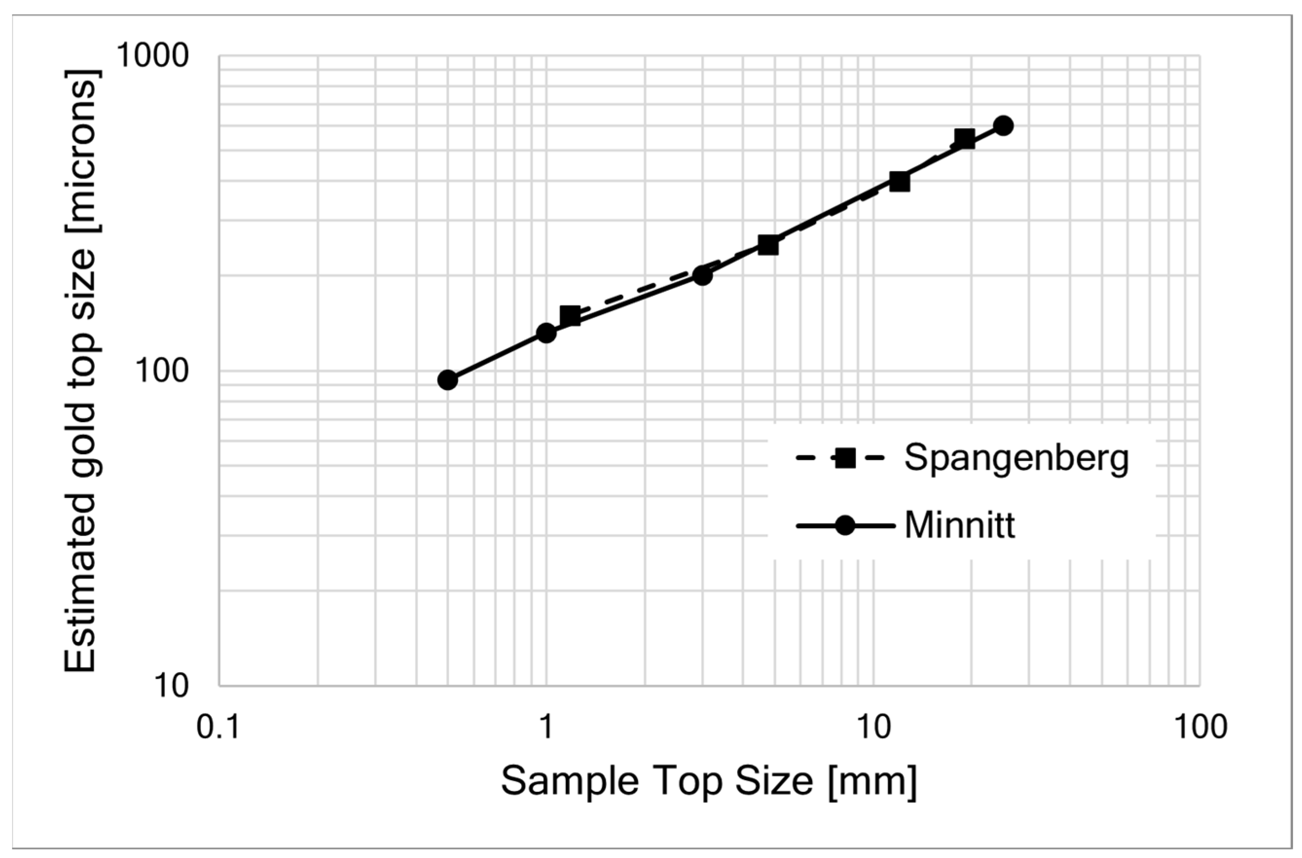
The same calculations can be made using Spangenberg’s data [11]. Both the Minnitt and Spangenberg data are plotted in Figure 1. The ore samples in both cases came from the same mine (Minnitt, private communication).

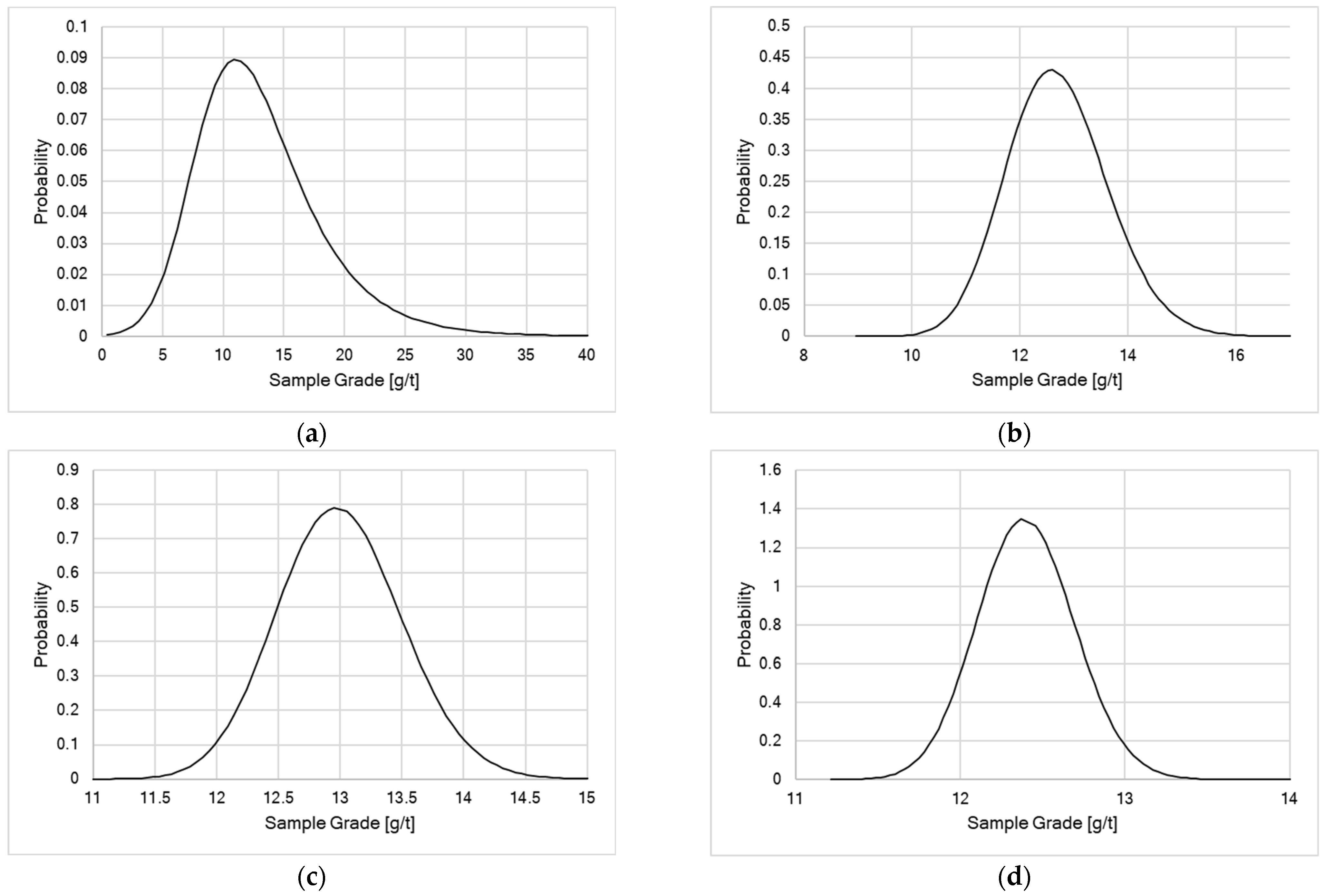
Having estimated the gold grain/cluster top size, it is now possible to calculate estimates of the full sampling distribution for the ore at the four top sizes using the characteristic function method using the assumptions regarding the effective size distribution and shape factor of the gold. These distributions, shown in Figure 2, are used to evaluate the sampling constants relative standard deviations for the distributions, and the maximum and minimum sample grades for comparison are used with the estimated 1.66 and 98.34 centiles of the distributions, respectively. These results are provided in

Table 4. Parameters for the data of Minnitt et al. [10] The values derived from the use of a Rosin–Rammler distribution for the gold cluster size and the particle size (n = 1.92), and grades are given in italics.

Particle Top Size (mm)	Cluster Top Size (μm)	Sampling Constant (g)	Grade (g/t)	RSD (%)	Min to Max Grade (g/t)
25	598	39.2 44.3	12.95	37.9 40.3	5.4 to 29.4 4.3 to 27.3
3.0	200	1.51 1.48	12.68	7.45 7.37	10.9 to 15.7 10.9 to 14.8
1.0	132	0.419 0.414	13.04	3.92 3.90	11.4 to 14.4 11.9 to14.1
0.5	93.7	0.158 0.155	12.41	2.40 2.38	11.1 to 14.0 11.8 to 13.1

.

The calculated distribution has taken the analytical variance correction into account, while those for the raw data have not, so the raw distribution is expected to be somewhat wider than the calculated distributions. In assessing the agreement, a confidence interval on the centile values for the raw data must be taken into consideration. Uncertainties on centile values can be large especially for low and high centiles. Given that the shape factor and size distribution factor were only roughly estimated, the agreement between the calculated distributions and the raw data is very good and demonstrates the utility of the method of estimation of the sampling distributions.

4. Discussion

The application of the Poisson characteristic function method to particulate sampling theory permits the completion of the particulate sampling theory developed prior to this work. The prior theory was based on Gy’s work [1,8], in which an expression for the sampling variance was provided. No higher moments of the sampling distribution (skewness etc.) were considered, and the importance of the fundamental basis of independent numbers of particle types following Poisson distributions was not used. The assay of a sample of a particulate material is a statistical quantity as it is the result of a random particle selection process. Full knowledge of any “statistic” requires a determination of its probability density function or, equivalently, all the moments of the distribution. This has not previously been possible, leaving the previous theory mathematically incomplete. The theory can now be deemed to be complete.

From a practical point of view, it is necessary to have a well-defined procedure that can be applied to an ore sample that provides results from which a comprehensive picture of the ore characteristics and its sampling properties can be derived. The sampling literature suggests a number of procedures, some of which are less useful than others. The enumeration and critique of these methods are beyond the scope of this paper.

There are a number of circumstances in which the full theory presented herein can be used to an advantage. First, for the sampling of gold ore, if the top size of the gold grains/clusters in the ore in a given sate of comminution can be estimated, the general model of a particulate material can be used to calculate the characteristic function for the ore using (17). This general expression can be specialized as appropriate for the nature of the ore as determined from microscopic studies. With reasonable assumptions about the deportment of the gold, no test work is necessary to begin the calculations of sampling distributions as a function of gold grade and sample mass. This simple process can be used to guide the development of sampling protocols for the ore, defining the masses of ore to be retained at any given top size of the ore that will reduce the skewness of sampling distributions to satisfactory levels. Confidence intervals for results cannot be correctly estimated if the sampling distribution is expected to be skewed; a reasonably estimated sampling distribution can be used to understand the manner in which sample assays will vary.

For the sampling of contaminated grains or other foodstuffs (mycotoxin contamination or adventitious contamination by genetically modified materials), sampling protocols can again be developed that control the nature of the sampling distribution and place confidence intervals on the results expected from sampling protocols using various sample masses. In these circumstances, it is critical to determine the expected skewness of results so that the confidence intervals are determined recognising the skewness. If only the sampling variance is known, confidence intervals are based on a normal distribution of results and such intervals may be far from the truth. The upper tail of a sampling distribution is critical in controlling the risk associated with a sampling protocol in which there is a maximum limit placed on the allowable concentration of contaminant in a consignment. The same is true when controlling the limits on contamination of some industrial minerals by, for example, asbestiform fibres.

It is the author’s view that the nature of the data set examined herein is the best basis for ore characterisation. The characterisation process should commence with a high amount of ore collected in such a way as to be consistent with the ore in a geotechnical domain, and the lot should be crushed to a top size of some tens of millimetres and carefully divided (rotary sample division) into several sublots of adequate mass. It is important that all subsamples at every stage be derived from original material and not from particular size fractions extracted from coarser material. One of these sublots should be further divided into nominally identical subsamples of some hundreds of grams (32 subsamples were formed for the data at hand, and 30 were then analysed to extinction). A further sublot should be crushed to a smaller top size and nominally identical subsamples analysed to extinction for all elements of interest. As smaller top sizes are used, the mass of the subsamples can be reduced, but not by so much that the spread of assays is swamped by analytical uncertainty. A stepwise process is required to balance manageable sizes of subsampled masses against the need to discern differences in subsampled assays relative to analytical uncertainty. The work should continue until a top-size to which the material is crushed permits a final pulverization to the top-size for the analytical aliquot. Multiple subsamples of appropriate mass at the analytical aliquot top size should be analysed to extinction so that the variance in assay at this size is discovered. Alternately, when the ore has been reduced to a particle size that can be mounted and sectioned for analysis in an automated scanning electron microscope (passing a 2 mm sieve), individual mineral particles can be mapped to show areas of different minerals within the particle. The mineral mounts are made for individual size fractions in the sample. These mineral maps on a particle-by-particle basis provide the compositional distribution information that is needed in the basic model of the ore as defined in Table 1 [12]. The amount of microscope work can be reduced for most ores by focusing on the two or three coarsest size fractions in the sample.

Test work of this nature must be closely controlled and not left to the staff of a commercial sample preparation and analysis facility to carry out as they see fit. All work must be supervised by a knowledgeable person who understands the importance of strictly following best practice and the procedures which must be closely specified. Appropriate sample preparation equipment must be available. Many commercial labs lack the correct equipment.

The assays from the various stages can then be analysed using the methods described in this paper. Having characterised the material, optimal sample preparation protocols can be devised in terms of top sizes to which to crush and sample masses to be retained at each top size in order to control the variance associated with the protocol. The variation of target mineral grain size will be evident from plots similar to Figure 1, which can be confidently interpolated.

5. Comments on Other Sources of Sampling Variance

The detailed theory provided here relates to sampling a particulate material from a larger lot of ore in a mechanically correct manner and is focused on the sampling variance that arises from differences in size and analyte content between the particles.

In the setting of process sampling from a flow of ore or from an orebody, a second source of variance comes into play due to the temporal or spatial variation (say between drill holes) of the ore properties and that source of variance is independent from that due to its particulate nature. While not the main objective of this paper, a summary of this additional component of variance is made here so that it is not ignored; it may indeed be the major source of variance when the particulate sampling is carried out in an industrial setting following a good design/protocol.

The appropriate analysis tool is time series analysis, in which a sequence of observed assays on some time base is taken to be a realization of a random function. This random function is a collection of random variables that are interrelated by a “covariance function”, which depends only on the difference in time (space) between observed values. Estimation of the covariance function is performed using maximum likelihood methods, which are the method of choice despite being computationally intensive. Other estimations rely on assumptions, which can seriously mislead the analysis.

Observations that are close together in time have a large covariance (tend to be similar in value), while those far apart in time have a low covariance (little similarity in value). The current sampling literature requires that observation times are based on a regular grid, but this need not be so and indeed limits the amount of information on the covariance function that can be derived from the data.

In practical terms, the sampling variance depends mostly on the first (short term and larger) part of the covariance function and this part of the function should be estimated with precision.

The analysis method and the interpretation of the data assumes the observed values are “stationary” with constant mean, variance about the mean, and covariance functions. Any long-term “drift” in the data mean has the effect of distorting the shape of the covariance function, making it appear to be linear when it is not. Consequently, observed data should be “detrended” by applying locally weighted regression methods to remove the longer-term drift. This step brings the data closer to stationarity, which it must have so as not to mislead the analysis; current literature in sampling ignores this requirement for stationarity and is consequently at risk of being misleading.

The variogram is much used in the analysis of spatially variable data and is directly related to the covariance function. The function was proposed by the early developers of geostatistics; for equally spaced data, it can be economically estimated. Maximum likelihood estimation methods for the covariance (variogram) are now preferred and practically available, and the observation times need not be equally spaced; equal spacing limits the amount of information on the covariance function carried by the data.

The current methods of analysis of time-wise process variation in sampling theory have been borrowed from early geostatistical methods and have retained the simplified methods in place at that time. They suffer from the following weaknesses:

• Data sets are not detrended;
• Unequally spaced data are forced to equal spacing to simplify variogram estimation;
• Uncertainties in the variogram estimates, derivable from the data, are ignored;
• Methods used to find periodicity within the variogram are not rigorous.
• These deficiencies lead to:
• Distortion of the variogram (covariance function) leading to incorrect estimation of sampling variance due to time variation;
• A conclusion that a covariance function is periodic when apparent periodicity is not statistically significant.

The appropriate methods of variogram/covariance function analysis are extensively dealt with by the author [9] with many quantitative illustrations. This second aspect of sampling theory has therefore been clarified with soundly based mathematics.

6. Conclusions

A consistent and sound statistical basis for particulate sampling theory has been proposed. The theory is based on a single simple assumption of Poisson-distributed numbers of particles in correct subsamples. It is shown to have practical application in calculating sampling distributions for even “difficult to sample” particulate materials, such as contaminated cereals, and should be capable of determining the sampling distribution for almost any particulate material.