Article

Retrieval of Subsurface Resistivity from Magnetotelluric Data Using a Deep-Learning-Based Inversion Technique

1
Geological Survey of Canada, 3303-33rd Street NW, Calgary, AB T2L 2A7, Canada
2
Geological Survey of Canada, 601 Booth Street, Ottawa, ON K1A 0E8, Canada
*
Author to whom correspondence should be addressed.
Minerals 2023, 13(4), 461; https://doi.org/10.3390/min13040461
Submission received: 17 February 2023 / Revised: 14 March 2023 / Accepted: 21 March 2023 / Published: 24 March 2023
(This article belongs to the Section Mineral Exploration Methods and Applications)

Abstract

:
Inversion is a fundamental step in magnetotelluric (MT) data routine analysis to retrieve a subsurface geoelectrical model that can be used to inform geological interpretations. To reduce the effect of non-uniqueness and local minimum trapping problems and improve calculation speeds, a data-driven mathematical method with a deep neural network was developed to estimate the subsurface resistivity. In this study, a deep learning (DL) inversion technique using a revised multi-head convolutional neural network (CNN) architecture was investigated for MT data analysis. We created synthetic datasets consisting of 100,000 random samples of resistivity layers to train the network’s parameters. The trained model was validated with independent noised datasets, and the predicted results displayed reasonable accuracy and reliability, which demonstrates the potential application of DL inversion for real-world MT data. The trained model was used to analyze MT data collected in the southwestern Athabasca Basin, Canada. The calculated results from the DL method displayed a detailed subsurface resistivity distribution compared to traditional iterative inversion. Since this approach can predict a resistivity model without multiple forward modeling operations after the CNN model is created, this framework is suitable to speed up the computation of multidimensional MT inversion for subsurface resistivity.

1. Introduction

An inverse problem is a process of predicting the causal input from the outcome of measurements, given a partial description of a physical law-based system. The application of inverse theory is widely applied in the science and engineering disciplines, such as geophysics and computer vision [1]. The inversion of magnetotelluric (MT) data is one such application that uses surface measurements of the Earth’s natural electric and magnetic fields as inputs to retrieve the subsurface resistivity structure for the interpretation of subsurface geology. The forward modeling procedure is based on the calculation of electromagnetic (EM) fields from a subsurface geoelectric model using numerical solutions of Maxwell’s equations [2,3,4]. Different inversion optimization methods, such as the non-linear conjugate gradient and Gauss–Newton method, have been studied [3,5,6]. The main principle of these approaches is using an iterative optimization technique to minimize the parametric function, including a data misfit function and a stabilizing function. Some useful software packages have been developed successfully for use by the MT community in academia and industry, such as Occam and ModEM [5,7].
Although there are some advantages inherent to traditional inversion methods, such as delivering details of the electrical structure of the subsurface, these inversion methods still face a few challenges. The first issue is that an initial physical model needs to be considered to reduce the possibility that the objective function may trap the search in a local minimum. Additionally, forward modeling, especially for 3D geoelectric structures, is numerically challenging, requiring significant computational resources despite recent advances to avoid lengthy computation times [8]. This issue is exacerbated for iterative inversion schemes that creep toward a final model using multiple forward computations. It must also be borne in mind that the non-linear inversion of band-limited non-precise data is unstable and non-unique [3,9]. Although regularization methods and physical constraints may be employed to stabilize the inverse solution, an alternative technique, such as deep learning (DL) that leverages modern GPU hardware and algorithms, could be investigated to assess its ability to replace traditional inversion techniques.
The DL method has matured in recent decades [10,11]. More recently, DL has received increased popularity in various disciplines due to leaps in computer hardware development that are ideally suited for the underlying DL algorithms [12,13,14,15]. As an increasingly popular method for data-driven inferences in geoscience disciplines, artificial neural networks (NN) have already demonstrated a considerable number of successful applications in different areas. For example, similarly to image segmentation in self-driving cars [16] and medical image analysis [14], an NN framework has been used to aid in the extraction of clay mineralogy and fracture mapping from scanning electron microscope images with U-net and DeepLab architecture [12,17], both of which are based on a convolutional neural network (CNN) approach. These architectures use several convolutional operation layers with modified structures and parameters. For optimization problems in geophysics, previous studies have shown that DL algorithms can be used to solve inverse problems. Kim and Nakata [1] and Russell [18] compared machine learning and geophysical inversion, showing that machine learning yields results with high spatial resolution. Das et al. [19] deployed CNN for seismic impedance inversion and demonstrated promise in the performance of more accurate, faster seismic reservoir characterizations in comparison to traditional inversion techniques. The DL inversion procedure is computationally instant after the model is created, which can improve inversion efficiency. To overcome the drawbacks of traditional EM inversion methods, it is worth investigating a DL architecture to retrieve the geoelectric structure of the subsurface. Moghadas [20], Puzyrev [21], and Puzyrev and Swidinsky [22] presented 1D inversion approaches of EM induction data, controlled source EM, and time domain EM (TEM) data using CNN models. These studies displayed impressive inversion results using a CNN architecture, which suggest the potential for CNN inversion for more widespread use in EM exploration. Liu et al. [23] presented a sample-compressed neural network algorithm for MT inversion and an adaptive clustering analysis algorithm for resistivity boundary demarcation, and Guo et al. [24] employed a supervised descent method (SDM) for 2D MT data inversion to reduce uncertainty. Conway et al. [25] applied a non-convolutional NN model to approximate the 3D MT forward method instead of resolving expensive forward functions, speeding up the inversion procedure and producing reasonable resistivity models. Further studies on MT inversion using CNN architecture are still necessary for obtaining deeper resistivity distributions and should be verified with a case study.
In this study, we revised the previous NN architecture to improve the model’s stability and estimate the subsurface resistivity distribution. Our main activities are the following: (1) to create and implement a multi-head CNN model based on U-net architecture, which uses measured MT apparent resistivity and phase data and facilitates working in a multi-scale context; (2) to update a CNN inversion workflow for dataset generation, model training, validation, and prediction, which makes the datasets cover a large range of possible resistivity variations; (3) to test the sensitivity of the model to noise and compare the results with the traditional MT inversion method; (4) to assess this CNN inversion method with the study of synthetic and real MT data from the Athabasca Basin. This study presents a novel scope of DL algorithm application for MT inversion and explores the critical task of training dataset generation and model framework, which was reflected in the sensitivity of noised data and real data results.

2. Methodology

2.1. MT 1D Forward Modeling

The MT method retrieves the subsurface distribution of electrical resistivity by measuring the variations of the EM field at the Earth’s surface, over which a source signal is assumed to be a naturally occurring, time-varying magnetic field and its induced electric field. The recorded electric and magnetic fields at the surface of the Earth contain resistivity information on the subsurface, and their ratio in frequency is termed an impedance tensor, Z ω = E ω H ω , where E is the electric field strength, H is defined as the magnetic field strength, and ω is the angular frequency [2,3]. The frequency-dependent tensor can be written in Cartesian coordinates.
E x E y = Z x x Z x y Z y x Z y y H x H y
Assuming that natural EM fields travel in terms of 1D resistivity media, the components of the impedance tensor can be simplified as follows:
Z x x = Z y y = 0 Z x y = Z y x
The apparent resistivity and phase are commonly used in 1D data analysis. The phase is the lag between the   E and H fields, whereas the apparent resistivity ( ρ a ) is a normalization of the field amplitudes and can be expressed as follows:
ρ a ω = 1 ω μ Z x y ω 2
where μ is the magnetic permeability.
It, therefore, represents an average resistivity between the Earth’s surface and skin depth
  δ = 2 ω μ σ
which is a function of conductivity   σ . Figure 1 shows the apparent resistivity and phase for various 1D models. The Occam1D forward modeling code is used to calculate the response of the three-layered resistivity models [26]. We can see that when the resistivity decreases, the phase is higher than 45°, and when the apparent resistivity increases, the phase switches to below 45°. With the dispersion relationship, the apparent resistivity and phase are coupled with causality. Based on this relation between apparent resistivity and phase, a consideration of both responses as input of the neural network will help reduce uncertainty and achieve a highly generalized DL model. For creating a CNN model for 1D MT inversion, the trained DL neural parameters will be calculated based on a group of randomly generated resistivity models. The simulated apparent resistivity and phase are gathered as the input and the resistivity model as the output for calculating the weight parameters during model training.

2.2. MT Inversion with CNN Architecture

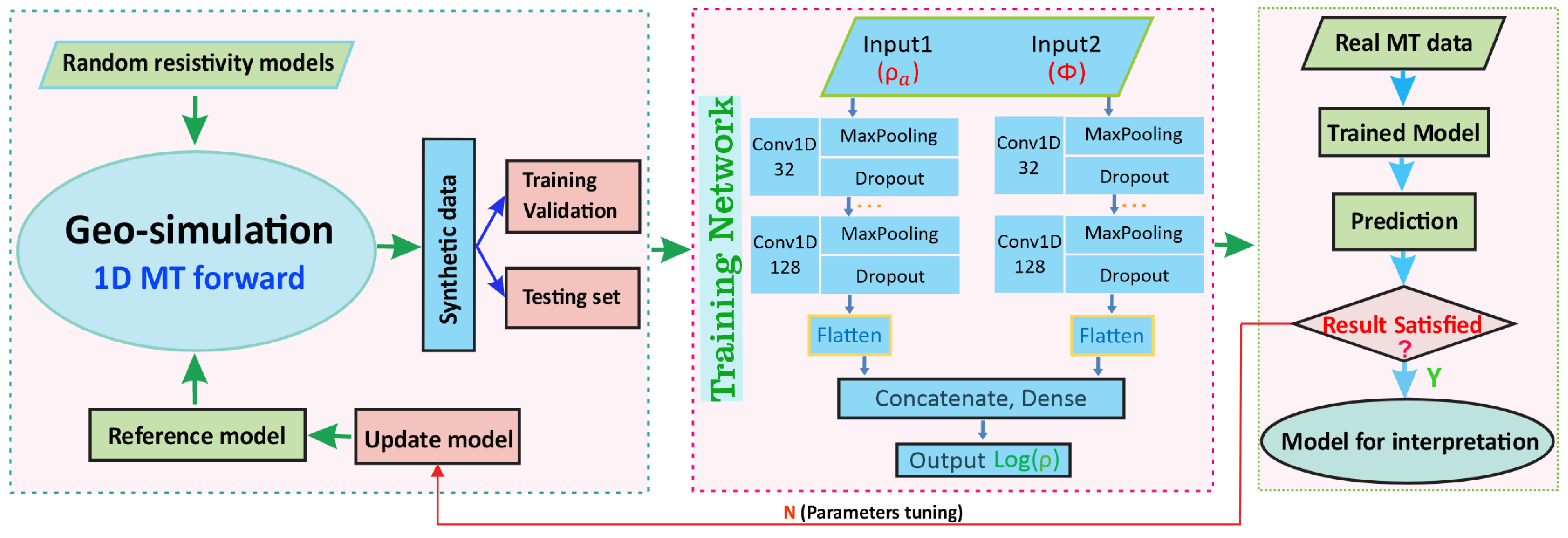
Geophysical inversion attempts to estimate the distribution of physical properties of the subsurface based on observed data. The proposed workflow in this study implements a DL algorithm with a revised U-net CNN model to predict the resistivity from the measured apparent resistivity and phase directly. Similarly to the common DL procedure, the flowchart in Figure 2 shows the major components and CNN architecture of an MT inversion consisting of three modules: data generation; neural network training and validation; and prediction.

2.2.1. Training Dataset Generation

The quantity and quality of the dataset for training the neural network model parameters are essential for prediction accuracy. As the left box in Figure 2 shows, the dataset (apparent resistivity ρ α and phase φ ) was generated using this workflow and split into a training set and validation set using an 80:20 ratio. The random resistivity models were created with a 50-layer model and a limited resistivity range of 1–104 Ωm. The resistivity distribution in each model was randomly generated with a maximum of 10 major anomalous continuous resistive or conductive zones. The thickness of the layers was fixed for all models and started at 20 m and increased in thickness to 10,000 m for the bottom-most layer. The maximum depth was 100 km. A total of 128 frequency points were calculated within a range of 0.001–100 Hz. The forward module in the Occam inversion package was used to calculate the apparent resistivity and phase [26]. The large amount of variably shaped resistivity models will cover most of the possible subsurface 1D geoelectric models without using any data augmentation methods. For this study, we generated 100,000 layered resistivity samples for model training and validation, which took about 40 min using a 56-core CPU desktop. The common logarithm of resistivity m = l o g 10 ρ was used as the targeted model parameters, and the input data x were standardized to value x ˜ using mean μ o and standard deviation σ o values when processing training [22,27].
x ˜ = x μ o σ o

2.2.2. CNN Inversion Framework

The most important part of this CNN inversion procedure is calculating the weight parameters of the neural network, which includes model training and validation. Since apparent resistivity and phase are different features and need to be input for training, the popular CNN approach, a multi-head architecture model, is employed for this study (Figure 2) [28,29]. Since only 128 frequency points were used for this model framework, a feature map with a convolution kernel size of three was used. The framework includes two parallel heads for feature analysis processing of standardized apparent resistivity and phase. Each head, which is at the top of the network, used an independent channel and was designed using similar 1D CNN layers but different weight values within neurons to extract features from the corresponding input; then, the interpretations of both heads were concatenated into one interpretation as a fully connected layer [28,29]. For each convolution layer, the number of filters increased from 32 to 128 with a rectified linear (ReLU) activation function and a stride of two, which is followed by 0.5 dropout and max-pooling layers. The ReLU is a linear function, f x = max 0 , x , which has the advantage of overcoming the vanishing gradient problem in comparison to the sigmoid function. The filter is an array vector as a feature detector; the stride is a parameter for controlling the filter’s movement; the max-pooling layer is a method for downsampling features by calculating the maximum value for each input patch, which is a subsection of input data; the dropout layer is a regularization method that sets some hidden layer neurons to zero randomly during each epoch, which means one cycle of model training with all the data. The main function of the dropout layer is to prevent model overfitting to get a better convergence of validation. The details regarding the definition and function of these NN layers are based on the Keras API [27]. The increased number of filters allows the NN to propagate contextual information to complex layers for better feature extraction. More details on the U-net CNN model can be found in Chen et al. [12] and Ronneberger et al. [14]. During the training and validation epochs, the network parameters are updated by minimizing the objective function. This is specified by the root mean squared error (RMSE) as the loss function metrics:
  RMSE = 1 n 1 n y i p r e y i m o d 2
where y i p r e is the predicted value, and y i m o d is the input model. The objective function of known resistivity models and their corresponding forward results is used to train the network with the Adam (adaptive moment estimation) optimization algorithm, which is an extension of the stochastic gradient descent for first-order gradient-based optimization that has recently seen broader adoption for DL applications [30]. Adam combines the advantages of both the adaptive gradient algorithm and the root mean square propagation such that it can deal with sparse gradients and non-stationary objectives. Python and some relevant DL open-source libraries, e.g., Tensorflow and Keras, are used for realizing the procedure [27,31], and MTpy and Occam1D packages are used for model generation and output display [32].

2.2.3. Model Test and Element Selection

The network’s model training and validation is a key step for calculating the model’s parameters and avoiding overfitting. In this study, model training took about five hours, while the iterative method for each station took two minutes of computation time with a batch size of sixty-four using one NVIDIA Quadro-P5000 GPU to reach stable accuracy. The model with the best validation loss is saved during a maximum of 150 epochs. Because CNN MT inversion is a data-driven technique, the model’s testing process is conducted to verify the reliability of the created model. During this procedure, the extra random resistivity models are generated with different parameters, such as layer thickness and kernel size, to test the trained CNN model. If the RMSE and the correlation coefficient of the test results are not satisfied, different resistivity models will be added for training the network. Although the general core neural of all network frameworks are similar, the difference in shapes and structures of the NN will affect the accuracy of the model’s prediction. Before starting model training, the selection of elements is a key component for high-accuracy prediction. In order to improve RMSE accuracy, different hyper-parameters (e.g., network structure, number of hidden layers, batch size, filter number and size, activation function, and optimization function) were adjusted during the model’s training period. The batch size affects the convergence speed and final validation accuracy. During the testing of different kernel sizes, a slightly larger kernel size (e.g., seven) will lead to a model with better noise tolerance but worse accuracy and less detail compared to the smaller kernel size (e.g., three). The activation function ReLU shows a more stable convergence than the linear operator. In addition, we also tested different learning rates for model updating. We chose four hidden layers for both contracting and expanding paths with a fixed kernel size of three for the final model. After the tests were verified, the same network architecture and weight parameters were saved and used in the rest of the program.

3. Synthetic Model Study

3.1. Results of the Synthetic Model

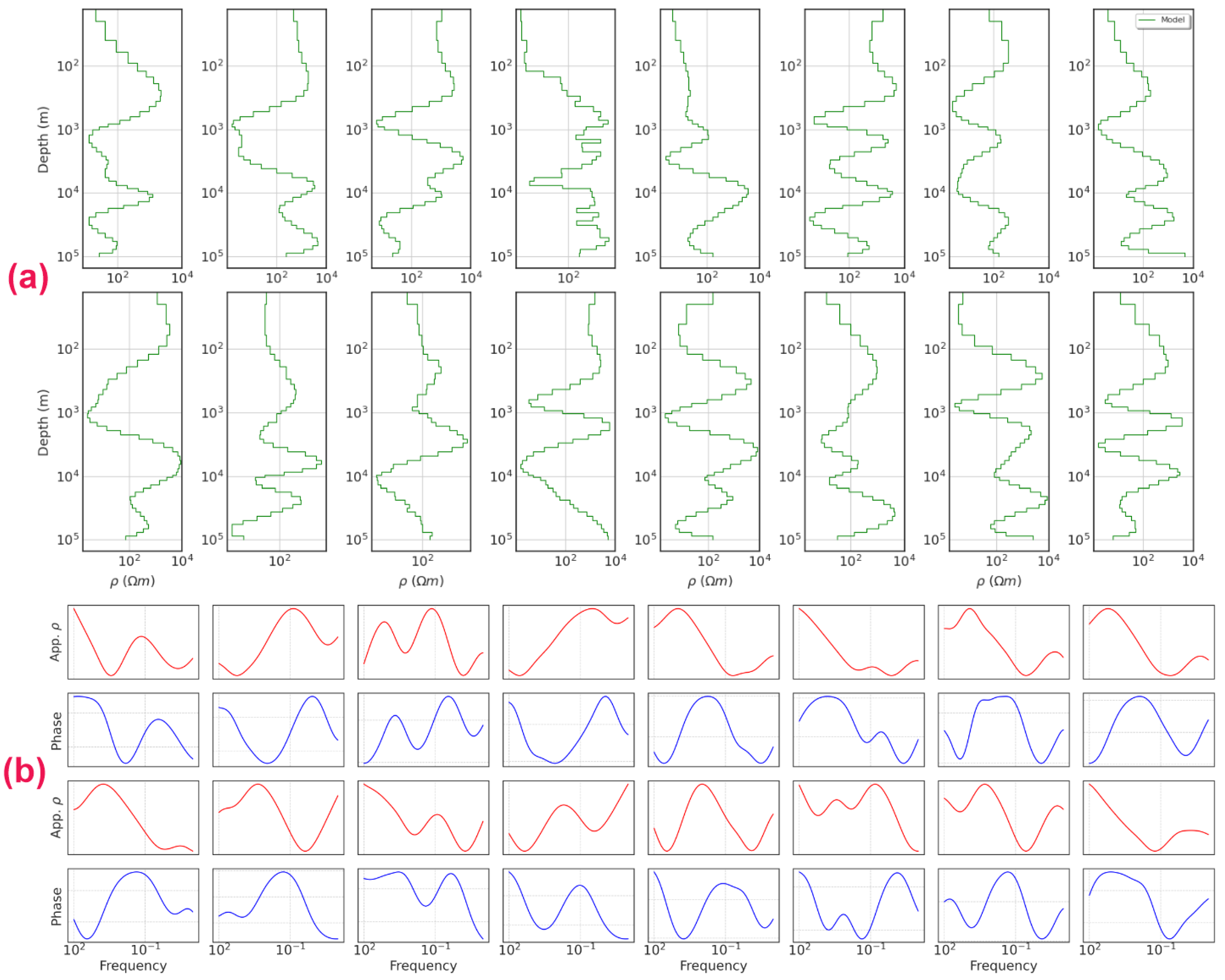
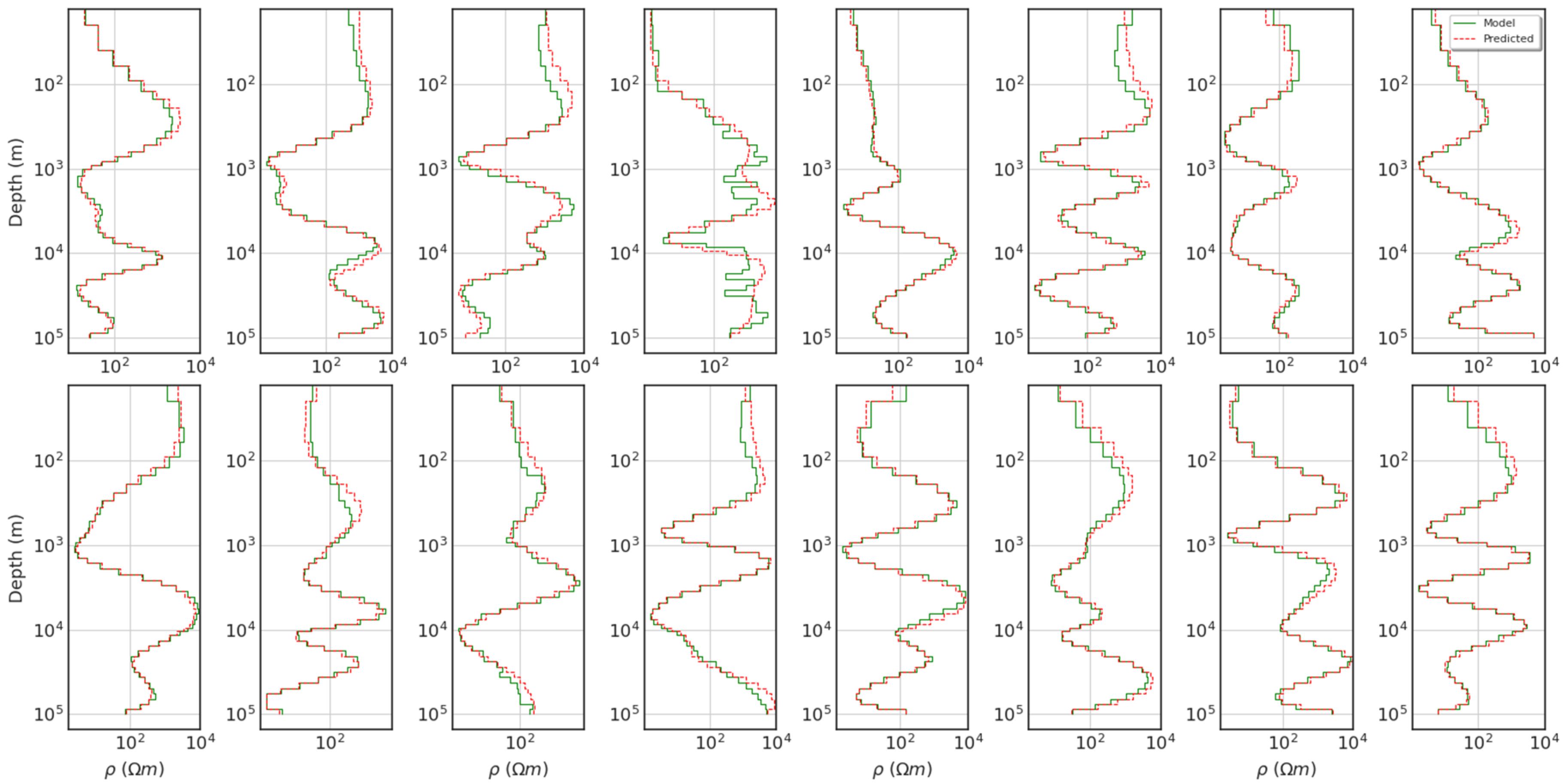
To evaluate the functionality and efficiency of the trained network model, we created synthetic models and calculated apparent resistivities and phases for model testing. The purpose of model testing is to demonstrate whether an accurate result can be obtained for a general resistivity distribution. The MTpy and Occam1D inversion packages were used to create the input files and conduct the forward modeling, respectively [5,32]. In Figure 3a, the sample data for model testing used similar criteria relative to the training dataset that was generated with a maximum of 10 major anomalous resistive or conductive layers. One can see the variation of resistivity models that cover different distributions and are diversified for creating a generalized network model. Figure 3b shows the forward apparent resistivity and phase (as input datasets). Figure 4 shows a comparison of the resistivity model and predicted inversion results with the trained CNN model. We can see that most predicted results identified the deep anomalies and displayed the desired trend in resistivity variations; however, a few predicted areas show significant bias, such as in the complex resistivity distribution zone (e.g., the fourth model on the top row). To compare the predicted results with the true values, both the normalized RMSE and correlation coefficient ( R ) from the model testing were calculated. In general, both values are within an acceptable range. Most misfits reach 0.05, and the R is greater than 0.97 (Table 1).
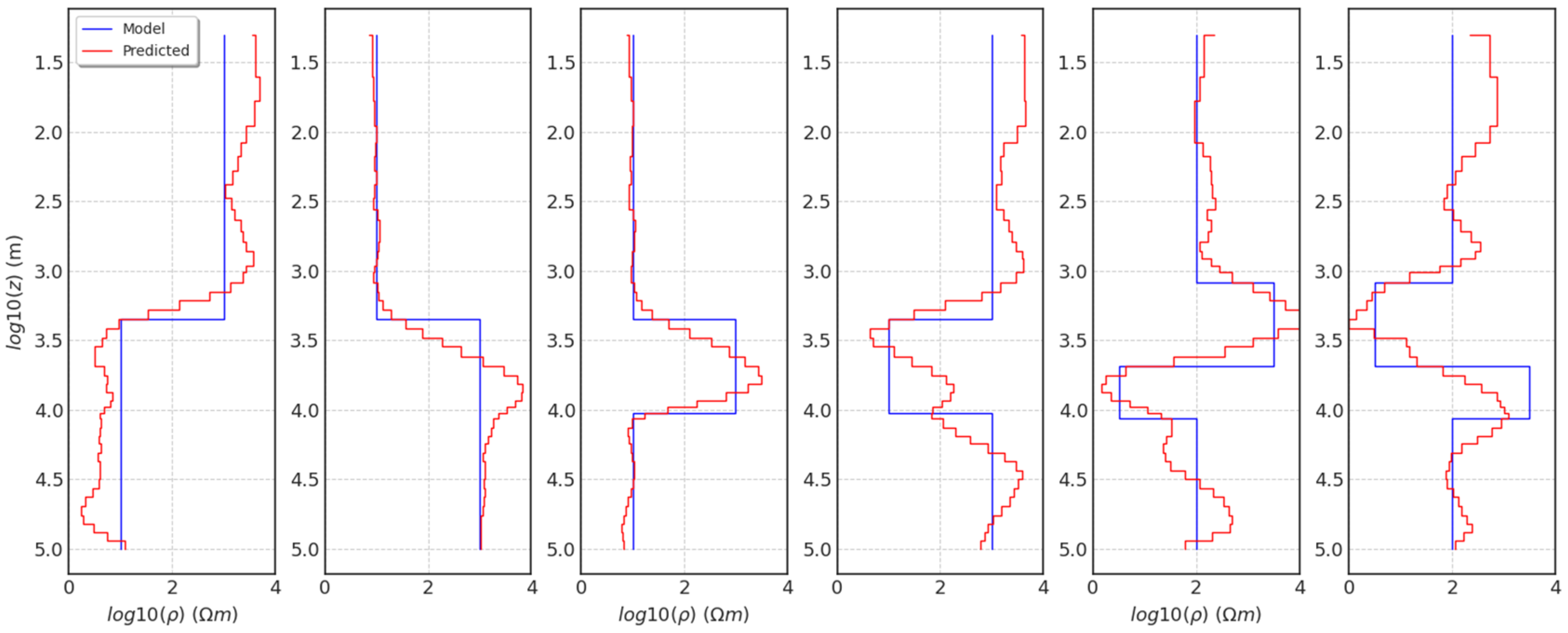
During the CNN model’s training and validation, we used 50-layer models with continuous variable resistivity at the boundary between layers. The non-continuous resistivity models and response were not added in model training, which might affect the predicted accuracy compared to non-continuous models. To further test the reliability of the model prediction, we created a few simplified models with discontinuous layer boundaries and compared the results with the CNN inversion (Figure 5). We can see that all predicted resistivity distributions are consistent with the true models and show the trend in spatial variations. Compared to the results of the continuous model (Figure 4), the bias with a non-continuous structure is larger. In general, the trained CNN model works well for both continuous and discontinuous structures.

3.2. Comparison with Traditional Iterative Inversion

To verify the accuracy of the proposed method, we compared the CNN-predicted results with a traditional deterministic inversion method, which takes an initial model and updates the resistivity model until the best fit is achieved with the observed data [5,26]. In this study, 300 synthetic data were randomly generated using 1D forward simulation. During the inversion, the same layer thickness was used, and the number of frequencies remained the same.
We calculated and plotted the statistic distribution of misfit RMSE and R based on testing of the synthetic models (Figure 6, Table 2). The figure shows that the misfit RMSE distribution peak (Figure 6 (left)) of the traditional inversion is higher than the CNN inversion, and in some cases, the correlation coefficient peak (Figure 6 (right)) is lower as well. We can also see that the results of traditional inversion reflect a larger variation than the CNN, and the quartile lines are wider than CNN inversion, which indicates that the trained CNN model produces geoelectric structures with less uncertainty. In general, the values of R and RMSE (Table 2) show that the predicted resistivity models using CNN inversion are better than the results calculated from traditional inversion. The peak values of calculated R are 0.981 and 0.968, and the RMSEs are 0.0455 and 0.0752, respectively.

3.3. Stability Test for Performance

In the study, the CNN architecture has been trained and validated with a noise-free dataset. To check the stability of this network in the presence of noise, the original resistivity and phase were distorted with noise using Equation (7). We added random noise to the simulated apparent resistivity and phase at different levels (3% and 5%). Noise was added according to the following formula:
D n = D + s · D m a x D m i n · r 0.5
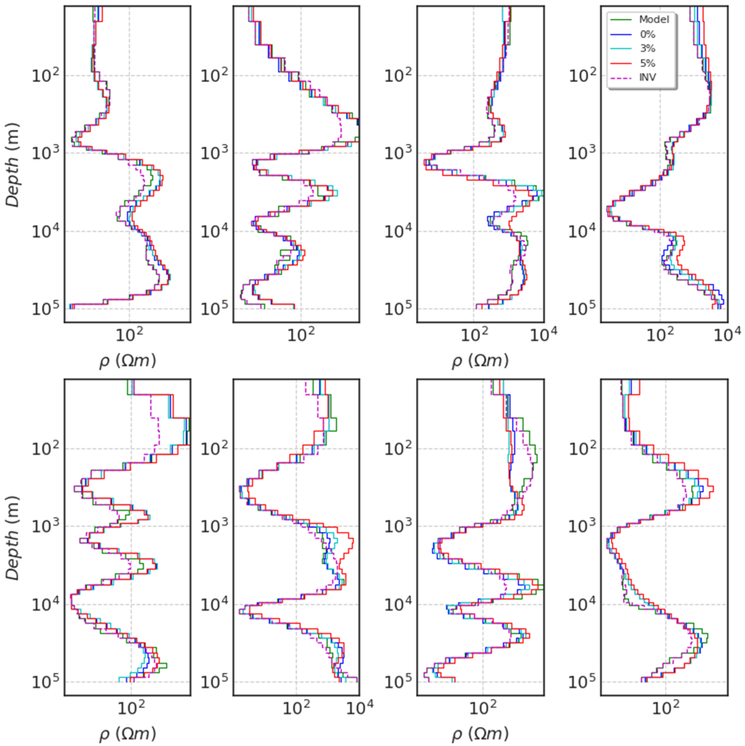
where D n is noised data, D is raw data, D m a x and D m i n are maximum and minimum of D , s is used to adjust noise magnitude, and r is a generated pseudo-random number. The noised datasets were loaded into the trained CNN model directly to calculate resistivity. In comparison to the true model, the eight inverted results show the correct trend in resistivity variations (Figure 7). As expected, the dataset with 5% noise exhibits a larger bias than the data with a 3% noise level; e.g., the fourth testing model is noised with [0%, 3%, and 5%], the R values are [0.9842, 0.9744, and 0.9692], and the RMSEs are [0.0549, 0.0722, and 0.1037]. In general, the output is stable in the presence of noise. In high-resistivity zones, the noise had a greater effect; however, by comparing the results with traditional inversion (INV), the trained CNN model can retrieve reliable results from noised data. In some samples (e.g., 2nd and 5th), the traditional inversion results show a larger bias than the output with noised data in shallow layers.

4. Application to Real Data

4.1. Geological Setting of the Study Area

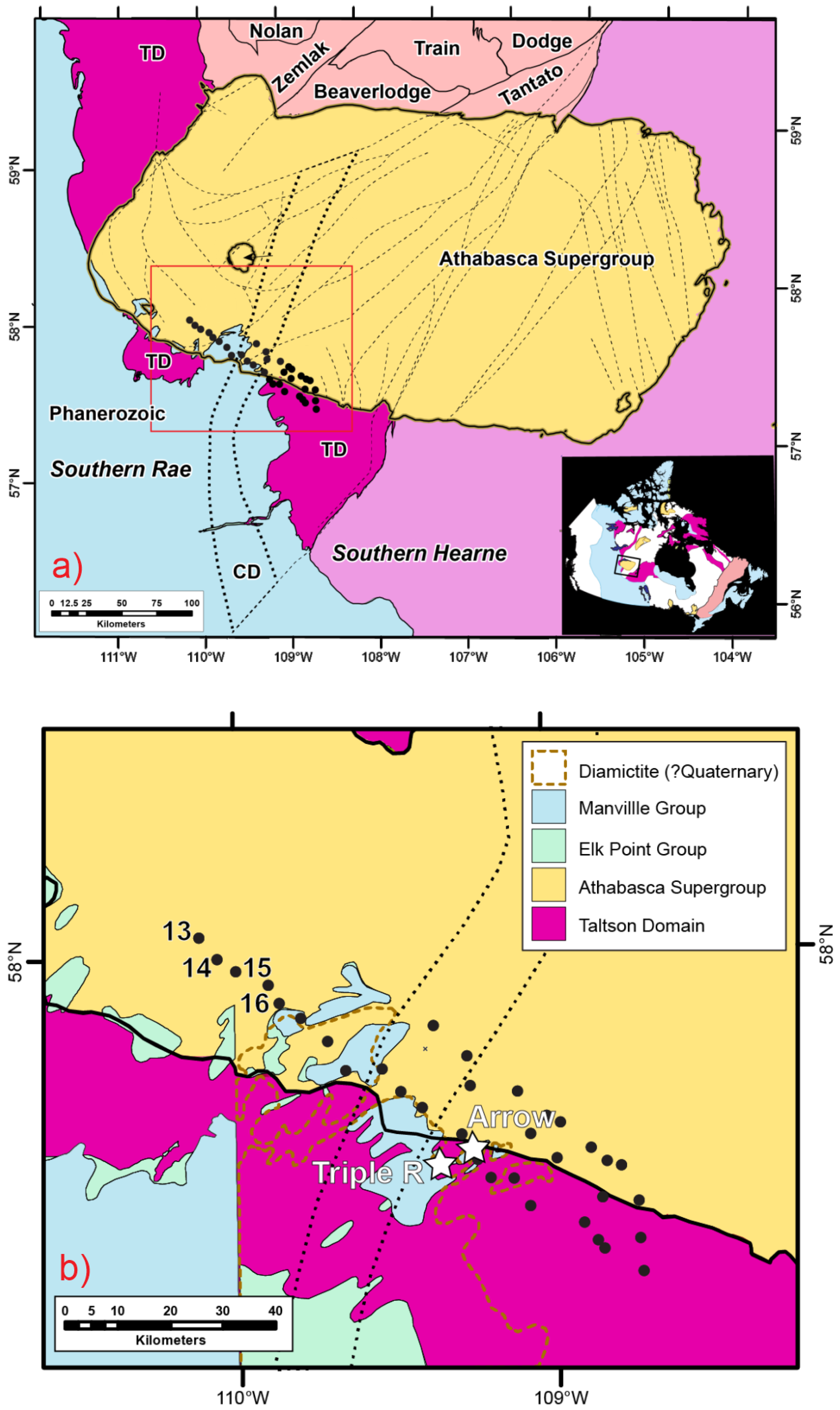
The Athabasca Basin (Figure 8a) straddles the border of Northern Saskatchewan and Alberta and is the premier region for uranium exploration in Canada, hosting the highest-grade deposits in the world. The study area is in the western Athabasca Basin (Figure 8b) where flat-lying Paleoproterozoic sedimentary rocks of the Athabasca Supergroup unconformably overlie Taltson Domain basement rocks. There is a large range in the electrical resistivity properties of the rocks in and below the Athabasca Basin; the sandstones and underlying orthogneisses and intrusive rocks are characterized by high resistivity, with resistivities greater than 5000 Ωm on average in the eastern Athabasca Basin; silicified fault zones have high resistivities; hydrothermal alteration haloes have elevated conductivities [33,34].

4.2. Real Data Inversion Results

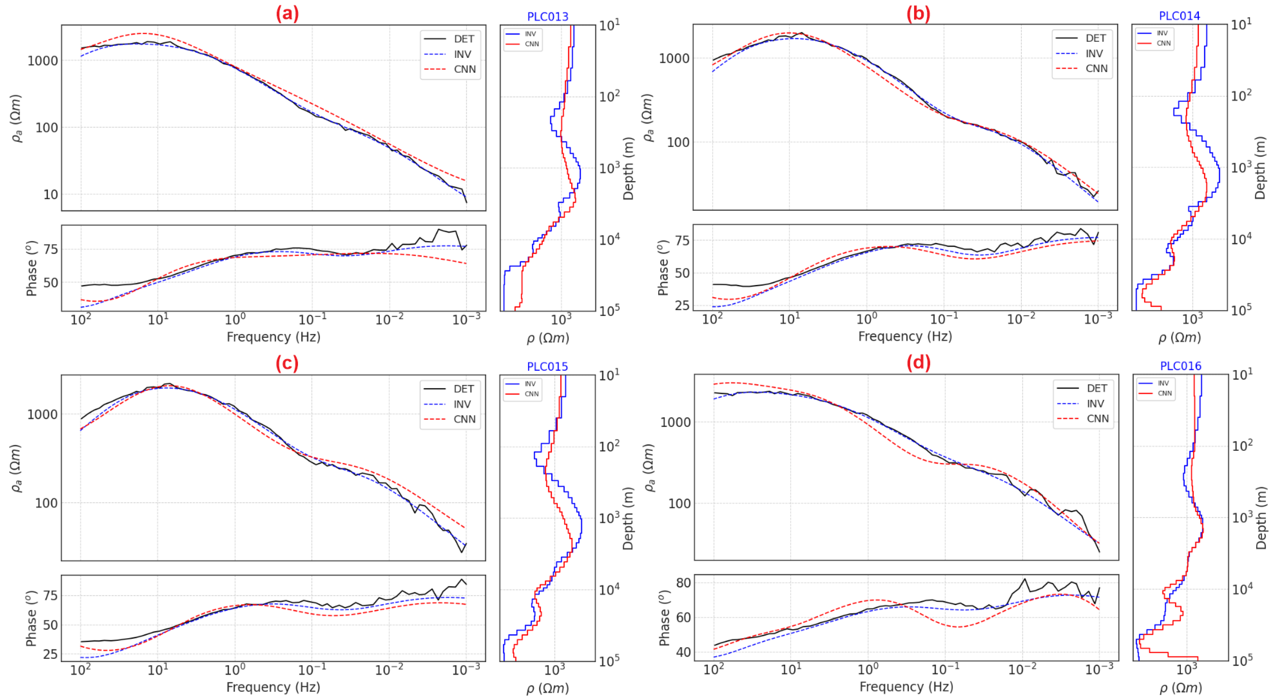
To visualize the lower crustal electrical properties, 34 broadband MT stations were collected using Phoenix Geophysics MTU-5A recorders along 2 northwest–southeast profiles transecting the PLC [37]. To test the accuracy of the trained 1D CNN model proposed in this study, four sites (PLC013, PLC014, PLC015, and PLC016; Figure 8b) were selected from the Athabasca dataset. Geologically, at these sites, upwards of ~750 m of resistive Athabasca Supergroup sedimentary rocks unconformably overlie Taltson Domain basement rocks with no major interpreted intersecting faults and, therefore, should broadly approximate a 1D Earth [36,38]. The determinant average of the impedance tensor at different frequencies was calculated for use in CNN model testing (Equation (8)) [39].
Z d e t = Z d e t e i d e t = Z x x Z y y Z x y Z y x
The predicted subsurface resistivity with the trained CNN model is presented in Figure 9. The dotted red line is the forward apparent resistivity and phase of the predicted resistivity model using the CNN inversion. We can see that most results predict the trend in the measured data. Compared to the results of the iterative inversion (blue), both methods identified the high resistivity zone around 1 km and displayed a similar trend in the resistivity distribution. We can see some differences in the resistivity models with the two methods in the near surface (<300 m) and mantle (>40 km) because of the effect of high noise levels in the data and the trend toward 3D geology at depth. Both the CNN and iterative inversions showed similar trends with respect to resistivity variations from 300 m to ~40 km. The prediction in the high-frequency zone shows a larger difference, potentially owing to static shift effects arising due to a resistive overburden at these sites. The deeper parts of the models are consistent across all four sites, where the resistivity decreases from 25 km to 40 km, coinciding with the boundary between lower crust and mantle, which is located at ~35 km depth in the study area [40]. Based on the inversion results in Figure 9, the inline classified resistivity section with site-to-site correlation is shown in Figure 10. The resistivity values are displayed in logarithmic space. The result of iterative inversion (Figure 10b) is a reference. Overall, the section shows a reasonable correlation in the resistivity variation between sites with both methods. The shallow layers show the resistivity increasing to a depth of ~1 km corresponding to the thickness of the Athabasca Supergroup cover [36]. The predicted results using the CNN inversion match the resistivity trend from a previous 2D inversion at some points, particularly at depths of less than 20 km [41].

5. Discussion

In this study, we investigated the possible use of DL for 1D MT data inversion. Compared to traditional inversion methods, the computation time required for CNN inversion is mainly spent on synthetic dataset generation and training/validation of the NN model parameters. Based on the computational resources available for this study (i.e., NVIDIA Quadro-P5000 GPU), the dataset generation and model training/validation stage is the most time-consuming part, taking approximately five hours. Because a trained model can be applied to all stations at the same time, the time taken to compute a predicted response is much faster since there is only a single calculation step. In contrast, traditional iterative convergence approaches with regularizing modeling constraints require updating the response after each iteration with computationally intensive forward modeling. Even for solving a 1D problem, traditional inversion will take around two minutes for each station depending on parameter settings. The advantage of CNN model prediction is that it is suitable for calculating many stations all at once. This study displayed the potential of CNN inversion to efficiently reconstruct subsurface resistivities with less computational requirements in general.
Despite the advantages of using the U-net CNN framework and its positive potential in MT inversion from the above analysis of synthetic and real data, there are a few limitations with respect to CNN inversion where improvements could be addressed. The generated dataset for training is not unlimited, which might lead to a bias of the related parameters in the network model. During the model training period, we considered a wide range of resistivity distributions so that better model parameters will be calculated and the predicted models would be closer to real-world data. To create a more generalized DL model, one approach is to make a model generator that covers even wider resistivity ranges so that the training datasets will be better suited to a wider variety of input data. During the synthetic model study, the trained model can predict more complex subsurface structures accurately after having added more layers to the architecture. In addition, a more complex network architecture could improve the accuracy of simulating the connection between physical models and MT-observed data. Because of limitations in computational power, we only considered four convolutional layers in each head for this U-shape neural network framework. By increasing hidden layers in the network architecture and the number of filters, it might reduce the noise effect of distorted data on the model. Finally, a different objective function with a stabilizer could be added to the training procedure. In general, optimizing training datasets, weights of layers, and a tuned objective function will make the DL inversion algorithm more powerful and efficient based on a given optimization strategy.
As the noise-tolerance testing showed, the predicted results show a larger bias at high noise levels. Updating the NN framework could be a solution and make the DL model process real-world noisy data more efficiently. Based on the results of the current study, it is possible that the application of this NN framework to anisotropic or 3D resistivity model inversion studies will be fruitful. With a similar NN architecture, the impedance and tipper will be used as inputs to train a CNN model for estimating the 3D resistivity model. Since numerous datasets are required for training and validation, the training period for 3D CNN inversion will require significant computational resources for both data generation and the calculation of weighted values of nodes. However, prediction processing with a trained model will be accomplished instantaneously, which is more efficient for skipping the optimization parameter adjustment during traditional iterative inversions. In this study, we demonstrated a proposed algorithm for implementing the optimization problem in MT 1D inversion with a CNN framework. Continuous research is still necessary to improve DL algorithms for solving high-dimensional MT data optimization problems.

6. Conclusions

In this study, 1D MT inversion using a revised U-net CNN architecture has been developed successfully. The merits of this technique are demonstrated by synthetic and real data testing. As a data-driven mathematical method, a trained network architecture can build a relationship between observed MT data and subsurface resistivity distributions and speed up the inversion procedure to derive reliable subsurface physical property distribution. The application of the trained network model to a noised synthetic test dataset produced satisfactory results and suggests that developing a network for complex geoelectric model inversion is feasible. Although containing some 2D and 3D geoelectrical structure and real-world noise, the predicted resistivity model using the MT stations from the western Athabasca Basin displayed reasonable geoelectric structure in comparison to results using traditional inversion algorithms. Thereby, the methodology study of DL-based inversion not only offers a prospective technique for geophysical data analysis but also presents a solution for obtaining regional subsurface resistivity distributions instantly for mineral resource assessment.

Author Contributions

X.L.: Methodology, software, and draft writing; J.A.C.: data collection, data curation, validation, revision, and funding acquisition; V.T.: data processing, data curation, geological interpretation, editing, and reviewing. All authors have read and agreed to the published version of the manuscript.

Funding

This work is fully funded by the Targeted Geoscience Initiative (TGI-6) program of Natural Resources Canada (Grant number: 340333).

Data Availability Statement

The generated datasets and real MT ‘.edi’ files in this study are available from the corresponding author upon request.

Acknowledgments

This study is funded by the TGI program of Natural Resources Canada. The authors are grateful to the two anonymous journal reviewers for constructive comments and suggestions. The authors thank research scientist Seyed Masoud Ansari at the Geological Survey of Canada for internal review and discussion during an early period of this study. The NRCan Contribution number is 20210009.

Conflicts of Interest

All co-authors declare that there are no potential conflict of interest in this study.

References

  1. Kim, Y.; Nakata, N. Geophysical inversion versus machine learning in inverse problems. Lead. Edge 2018, 37, 894–901. [Google Scholar] [CrossRef]
  2. Ward, S.H.; Hohmann, G.W. Electromagnetic Theory for Geophysical Applications. In Electromagnetic Methods in Applied Geophysics-Theory; Society of Exploration Geophysicists: Tulsa, OK, USA, 1988; Volume 1, p. 201. [Google Scholar]
  3. Zhdanov, M.S. Geophysical Inverse Theory and Regularization Problems; Elsevier Science: Amsterdam, The Netherlands, 2002; p. 214. [Google Scholar]
  4. Craven, J.A.; Farquharson, C.G.; Mackie, R.L.; Siripunvaraporn, W.; Tuncer, V.; Unsworth, M.J. A comparison of two- and three-dimensional modelling of audio-magnetotelluric data collected at the world’s richest uranium mine, Saskatchewan, Canada. In Proceedings of the 18th International Workshop on Electromagnetic Induction in the Earth, El Vendrell, Spain, 17–23 September 2006; p. 1. [Google Scholar]
  5. Constable, S.C.; Parker, R.L.; Constable, C.G. Occam’s inversion: A practical algorithm for generating smooth models from electromagnetic sounding data. Geophysics 1987, 52, 289–300. [Google Scholar] [CrossRef]
  6. Egbert, G.D.; Kelbert, A. Computational recipes for electromagnetic inverse problems. Geophys. J. Int. 2012, 189, 251–267. [Google Scholar] [CrossRef] [Green Version]
  7. Kelbert, A.; Meqbel, N.; Egbert, G.D.; Tandon, K. ModEM: A modular system for inversion of electromagnetic geophysical data. Comput. Geosci. 2014, 66, 40–53. [Google Scholar] [CrossRef]
  8. Ansari, S.; Schetselaar, E.; Craven, J.; Farquharson, C. Three-dimensional magnetotelluric numerical simulation of realistic geologic models. Geophysics 2020, 85, E171–E190. [Google Scholar] [CrossRef]
  9. Zhdanov, M.S.; Wan, L.; Gribenko, A.; Cuma, M.; Key, K.; Constable, S. Large-scale 3D inversion of marine magnetotelluric data: Case study from the Gemini prospect, Gulf of Mexico. Geophysics 2011, 76, F77–F87. [Google Scholar] [CrossRef]
  10. Fukushima, N. A self-organizing neural network model for a mechanism of pattern recognition unaffected by shift in position. Biol. Cybern. 1980, 36, 193–202. [Google Scholar] [CrossRef]
  11. Hochreiter, S. The Vanishing Gradient Problem During Learning Recurrent Neural Nets and Problem Solutions. Int. J. Uncertain. Fuzziness Knowl.-Based Syst. 1998, 6, 107–116. [Google Scholar] [CrossRef] [Green Version]
  12. Chen, Z.; Liu, X.; Yang, J.; Little, E.; Zhou, Y. Deep learning-based method for SEM image segmentation in mineral characterization, an example from Duvernay Shale samples in Western Canada Sedimentary Basin. Comput. Geosci. 2020, 138, 104450. [Google Scholar] [CrossRef]
  13. Long, J.; Shelhamer, E.; Darrell, T. Fully Convolutional Networks for Semantic Segmentation. arXiv 2014, arXiv:1411.4038. Available online: https://people.eecs.berkeley.edu/~jonlong/long_shelhamer_fcn.pdf (accessed on 14 November 2014).
  14. Ronneberger, O.; Fischer, P.; Brox, T. U-net: Convolutional networks for biomedical image segmentation. In Medical Image Computing and Computer-Assisted Intervention (MICCAI); LNCS; Springer: Berlin/Heidelberg, Germany, 2015; Volume 9351, pp. 234–241. [Google Scholar]
  15. Roy, A.G.; Navab, N.; Wachinger, C. Concurrent Spatial and Channel ‘Squeeze & Excitation’ in Fully Convolutional Networks. In Medical Image Computing and Computer Assisted Intervention—MICCAI 2018; Lecture Notes in Computer Science; Springer: Cham, Switzerland, 2018; Volume 11070. [Google Scholar] [CrossRef] [Green Version]
  16. Paszke, A.; Chaurasia, A.; Kim, S.; Culurciello, E. Enet: A deep neural network architecture for real-time semantic segmentation. arXiv 2016, arXiv:1606.02147. [Google Scholar]
  17. Chen, L.C.; Papandreou, G.; Schroff, F.; Adam, H. Rethinking Atrous Convolution for Semantic Image Segmentation. arXiv 2017, arXiv:1706.05587. [Google Scholar]
  18. Russell, B. Machine learning and geophysical inversion; a numerical study. Lead. Edge 2019, 38, 512–519. [Google Scholar] [CrossRef]
  19. Das, V.; Pollack, A.; Wollner, U.; Mukerji, T. Convolutional neural network for seismic impedance inversion. Geophysics 2019, 84, R869–R880. [Google Scholar] [CrossRef]
  20. Moghadas, D. One-dimensional deep learning inversion of electromagnetic induction data using convolutional neural network. Geophys. J. Int. 2020, 222, 247–259. [Google Scholar] [CrossRef]
  21. Puzyrev, V. Deep learning electromagnetic inversion with convolutional neural networks. Geophys. J. Int. 2019, 218, 817–832. [Google Scholar] [CrossRef] [Green Version]
  22. Puzyrev, V.; Swidinsky, A. Inversion of 1D frequency- and time-domain electromagnetic data with convolutional neural networks. Comput. Geosci. 2021, 149, 104681. [Google Scholar]
  23. Liu, W.; Lü, Q.; Yang, L.; Lin, P.; Wang, Z. Application of Sample-Compressed Neural Network and Adaptive-Clustering Algorithm for Magnetotelluric Inverse Modeling. IEEE Geosci. Remote Sens. Lett. 2020, 18, 1540–1544. [Google Scholar] [CrossRef]
  24. Guo, R.; Li, M.; Yang, F.; Xu, S.; Abubakar, A. Application of supervised descent method for 2D magnetotelluric data inversion. Geophysics 2020, 85, WA53–WA65. [Google Scholar] [CrossRef]
  25. Conway, D.; Alexander, B.; King, M.; Heinson, G.; Kee, Y. Inverting magnetotelluric responses in a three-dimensional earth using fast forward approximations based on artificial neural networks. Comput. Geosci. 2019, 127, 44–52. [Google Scholar] [CrossRef]
  26. Constable, S.C.; Weiss, C.J. Mapping thin resistors and hydrocarbons with marine EM methods: Insights from 1D modeling. Geophysics 2006, 71, G43–G51. [Google Scholar] [CrossRef] [Green Version]
  27. Chollet, F. Keras. Available online: https://keras.io (accessed on 14 November 2015).
  28. Canizo, M.; Triguero, I.; Conde, A.; Onieva, E. Multi-head CNN–RNN for multi-time series anomaly detection: An industrial case study. Neurocomputing 2019, 363, 246–260. [Google Scholar] [CrossRef]
  29. Khan, Z.N.; Ahmad, J. Attention induced multi-head convolutional neural network for human activity recognition. Appl. Soft Comput. 2021, 110, 107671. [Google Scholar] [CrossRef]
  30. Kingma, D.P.; Ba, J. Adam: A method for stochastic optimization. arXiv 2017, arXiv:1412.6980. [Google Scholar]
  31. Abadi, M.; Barham, P.; Chen, J.; Chen, Z.; Davis, A. Tensorflow: A system for large-scale machine learning. Oper. Syst. Des. Implement. (OSDI) 2016, 16, 265–283. [Google Scholar]
  32. Krieger, L.; Peacock, J.R. MTpy: A Python toolbox for magnetotellurics. Comput. Geosci. 2014, 72, 167–175. [Google Scholar] [CrossRef]
  33. Craven, J.A.; McNeice, G.; Powell, B.; Koch, R.; Annesley, I.R.; Wood, G.; Mwenifumbo, C.J.; Unsworth, M.J.; Xiao, W. Audio-magnetotelluric studies at the McArthur River mining camp and Shea Creek area, northern Saskatchewan. Bull.-Geol. Surv. Can. 2007, 588, 413–424. [Google Scholar]
  34. Farquharson, C.G.; Craven, J.A. Three-dimensional inversion of magnetotelluric data for mineral exploration: An example from the McArthur River uranium deposit, Saskatchewan, Canada. J. Appl. Geophys. 2009, 68, 450–458. [Google Scholar] [CrossRef]
  35. Jefferson, C.W.; Thomas, D.J.; Gandhi, S.S.; Ramaekers, P.; Delaney, G.; Brisbin, D.; Cutts, C.; Quirt, D.; Portella, P.; Olson, R.A. Unconformity-associated uranium deposits of the Athabasca Basin, Saskatchewan and Alberta. Geol. Surv. Can. Bull. 2007, 588, 23–67. [Google Scholar]
  36. Tschirhart, V.; Pehrsson, S.; Card, C.; Potter, E.G.; Powell, J.; Pană, D. Interpretation of buried basement in the southwestern Athabasca Basin, Canada, from integrated geophysical and geological datasets. Geochem. Explor. Environ. Anal. 2021, 21, geochem2019-061. [Google Scholar] [CrossRef]
  37. Tschirhart, V.; Potter, E.; Powell, J.; Roots, E.; Craven, J. Deep geological controls on formation of the highest-grade uranium deposits in the world: Magnetotelluric imaging of unconformity-related systems from the Athabasca Basin, Canada. Geophys. Res. Lett. 2022, 49, e2022GL098208. [Google Scholar] [CrossRef]
  38. Caldwell, T.G.; Bibby, H.M.; Brown, C. The magnetotelluric phase tensor. Geophys. J. Int. 2004, 158, 457–469. [Google Scholar] [CrossRef] [Green Version]
  39. Smirnov, M.Y.; Pedersen, L.B. Magnetotelluric measurements across the Sorgenfrei-Tornquist Zone in southern Sweden and Denmark. Geophys. J. Int. 2009, 176, 443–456. [Google Scholar] [CrossRef]
  40. Schetselaar, E.M.; Snyder, D.B. National Database of MOHO Depth Estimates from Seismic Refraction and Teleseismic Surveys. In Geological Survey of Canada, Open File 8243; Natural Resources Canada: Ottawa, ON, Canada, 2017; 14p. [Google Scholar] [CrossRef]
  41. Potter, E.G.; Tschirhart, V.; Powell, J.W.; Kelly, C.J.; Rabiei, M.; Johnstone, D.; Craven, J.A.; Davis, W.J.; Pehrsson, S.; Mount, S.M.; et al. Targeted Geoscience Initiative 5: Integrated Multidisciplinary Studies of Unconformity-Related Uranium Deposits from the Patterson Lake Corridor, Northern Saskatchewan. In Geological Survey of Canada, Bulletin 615; Natural Resources Canada: Ottawa, ON, Canada, 2020; 37p. [Google Scholar]
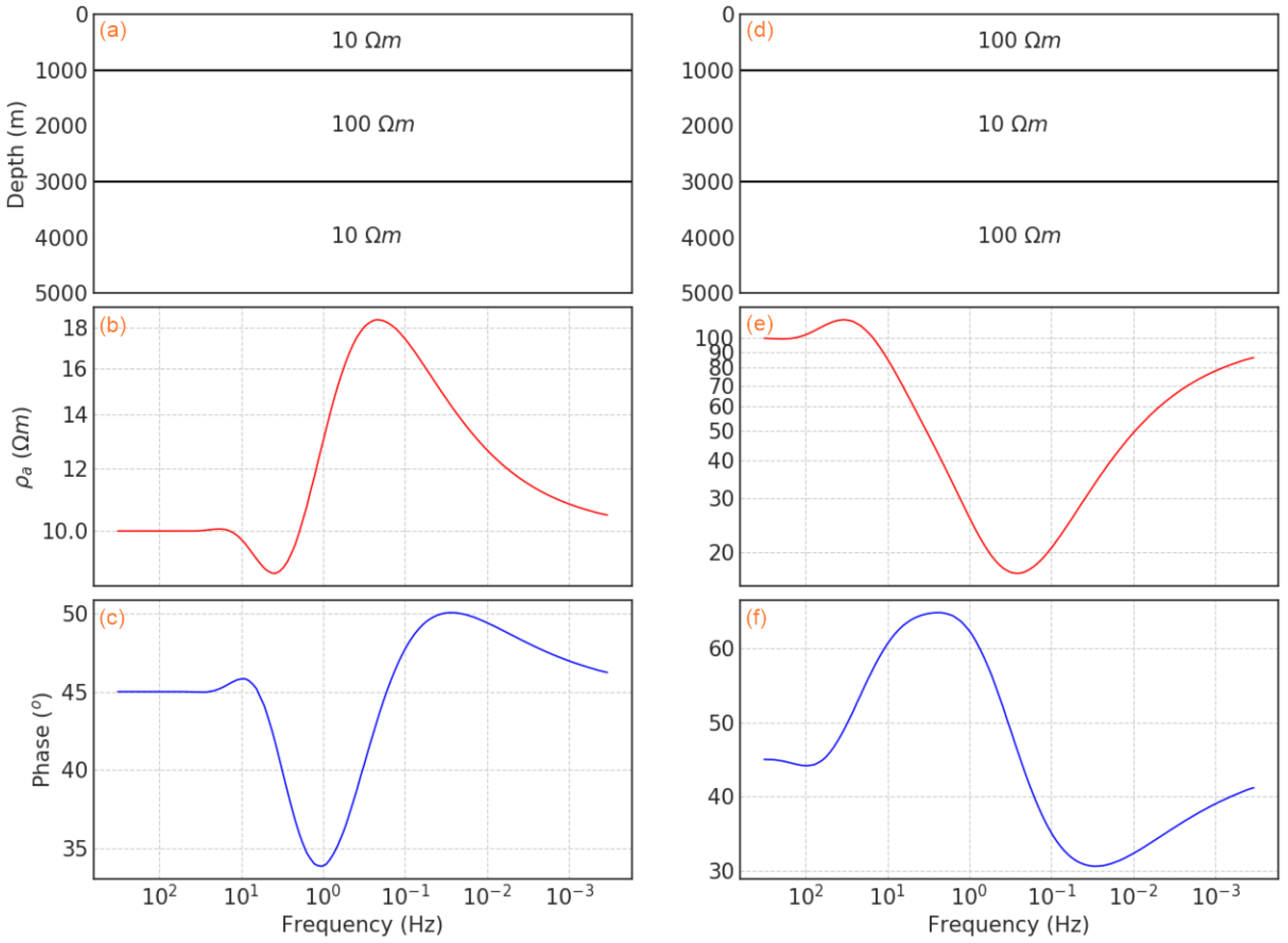
Figure 1. Synthetic model parameters (a,d) and its forward model curves showing the variation of apparent resistivity (b,e) and phase (c,f) on the Earth’s surface.
Minerals 13 00461 g001
Figure 2. A schematic workflow of the MT CNN inversion used in this study (left: resistivity model generation and forward response. Paired datasets are split for model training and validation; middle: A schematic network architecture displaying input and output for optimizing model parameters. More details of the U-net structure can be found in [12,14]; right: With a trained NN model, the datasets are used as inputs to calculate resistivity).
Minerals 13 00461 g002
Figure 3. (a) Samples of generated synthetic models that are selected randomly from the testing datasets; (b) calculated apparent resistivity and phase from the synthetic geoelectric models.
Minerals 13 00461 g003
Figure 4. Comparison of calculated resistivity with testing datasets in Figure 3a (green solid line is the true model; red dashed line is the predicted resistivity with a trained CNN model).
Minerals 13 00461 g004
Figure 5. Comparison of predicted resistivity with CNN inversion and true layered resistivity models.
Minerals 13 00461 g005
Figure 6. Violin plot of statistic distributions based on 300 results using CNN and traditional iterative inversion (INV).
Minerals 13 00461 g006
Figure 7. CNN inversion results of 8 synthetic samples at different noise levels (0%, 3%, and 5%) and iterative inversion (INV) results.
Minerals 13 00461 g007
Figure 8. (a) Simplified geological map of the Athabasca Basin outlining the location of (b) by a red box. Clearwater Domain (CD) is outlined by black dotted line, and the location of structures from Jefferson et al. [35] is plotted as black dashed lines. TD = Taltson Domain; (b) geological map of the Patterson Lake corridor MT survey area. Location of MT stations plotted as black dots; location of uranium deposits labeled by white stars (modified from Tschirhart et al. [36]).
Minerals 13 00461 g008
Figure 9. The plots of selected sites: (a) site PLC013, (b) site PLC014, (c) site PLC015, and (d) site PLC016. In the subplot of each site: left top panel: comparison of apparent resistivity between the determinant and 1D modeling response; left bottom panel: comparison of phase between determinant and 1D modeling response; right panel: predicted resistivity with a CNN model and traditional iterative inversion.
Minerals 13 00461 g009
Figure 10. Inline classified resistivity sections of four calculated 1D models with CNN inversion (a) and iterative inversion (b), which show the correlations of resistivity variations.
Minerals 13 00461 g010
Table 1. RMSE and R of selected model testing results shown in Figure 4.
ID12345678910111213141516
RMSE0.03160.05390.07080.12360.01930.05740.04990.03630.02910.04740.05190.05180.04740.04140.03410.0330
R 0.99610.99170.97700.91390.99810.98230.98950.99210.99600.98140.98600.99040.98690.99340.99610.9943
Table 2. The calculated R and RMSE using CNN and iterative inversion with 300 models.
Inversion MethodsCorrelation Coefficient (Peak)Misfit RMSE (Peak)
CNN0.9810.0455
Traditional Inversion0.9670.0752
Disclaimer/Publisher’s Note: The statements, opinions and data contained in all publications are solely those of the individual author(s) and contributor(s) and not of MDPI and/or the editor(s). MDPI and/or the editor(s) disclaim responsibility for any injury to people or property resulting from any ideas, methods, instructions or products referred to in the content.