Machine Learning Algorithms for Semi-Autogenous Grinding Mill Operational Regions’ Identification

Abstract

Energy consumption represents a significant operating expense in the mining and minerals industry. Grinding accounts for more than half of the mining sector’s total energy usage, where the semi-autogenous grinding (SAG) circuits are one of the main components. The implementation of control and automation strategies that can achieve production objectives along with energy efficiency is a common goal in concentrator plants. However, designing such controls requires a proper understanding of process dynamics, which are highly complex, coupled, and have non-deterministic components. This complex and non-deterministic nature makes it difficult maintain a set-point for control purposes, and hence operations focus on an optimal control region, which is defined in terms of desirable behavior. This paper investigates the feasibility of employing machine learning models to delineate distinct operational regions within in an SAG mill that can be used in advanced process control implementations to enhance productivity or energy efficiency. For this purpose, two approaches, namely k-means and self-organizing maps, were evaluated. Our results show that it is possible to identify operational regions delimited as clusters with consistent results.

1. Introduction

The mining industry plays an important role in the supply chain of critical minerals for the development of modern technologies; however, in recent years, the increased production costs along with lower ore grades have generated an interest in finding strategies to reduce operating costs and increase productivity. Within the mining process, the ore size reduction stage or comminution represents the largest energy consumption, and the operation of semi-autogenous grinding (SAG) circuits is commonly responsible for a high percentage of this power consumption [1].

The development of automation strategies to generate adequate production while reducing the energy consumption has been favored by the implementation of digital transformation tools in the mining industry [2]. These tools allow for a better understanding of the input/output relations in the process, which is an essential step in the development of control strategies. Artificial intelligence (AI) has proven a valuable tool for grinding representation, particularly in the area of the generation of SAG mill models suitable to be used for process control purposes. However, properly characterizing SAG mill dynamics is challenging, given that it has a largely nonlinear behavior, with coupled dynamics, and considerable delays [3,4], which is mainly due to the intrinsic variability in the treated ore. To overcome the challenge of SAG mill modeling, several research works have considered the use of AI-based tools to study the relationship among the SAG mill operational variables. In [5,6], the correlation between acoustic emissions, hardness, and feed size in SAG mills was studied using machine learning models. In [7], a deep learning approach to study mineral hardness and predict related values is presented. Ref. [8] demonstrated the efficacy of an SVM-NARMAX model in predicting the fill levels in SAG mills by incorporating historical error information. The work [9] encompassed a convolutional neural network (CNN) approach for monitoring grinding circuits. Ref. [10] utilized back propagation (BP) neural network models to evaluate the effective processing throughput of SAG mills. These studies collectively underscore the substantial impact of ML and AI approaches to study SAG mill operation.

Relevant research efforts have also been devoted to the study of energy consumption and its prediction based on the behaviors of other operational variables. Input–output models for predicting power consumption using a combination of genetic algorithms and neural networks (GANNs) were studied in [11] with favorable results. In [12], the authors developed a model for predicting energy consumption in SAG mills using machine learning (ML) and deep learning (DL) methods. An AI-driven approach was developed in [13], where a model based on gene expression programming (GEP) is used to predict the power of SAG mills’ consumption; Ref. [14] introduced a data-driven, multi-regime method for energy prediction. Ref. [15] compared different machine learning models to predict energy consumption in SAG mills, determining that deep learning provided one of the most promising results. The study in [16] reached a similar conclusion.

Aside from generating models used for representation and decision-making, the use of machine learning has also provided tools for improving control strategies. See [17] for an implementation using decision tree algorithms, Ref. [18] for intelligence-based hybrid approaches, and Ref. [19] where a compelling case study is provided that leverages machine learning techniques to enhance SAG mill productivity indicators such as production and energy consumption. A great review on this subject can be found in [20], where a rigorous discussion on the topic is provided. It is important to mention that the implementation of control and optimization strongly relies on the use the proper representation, particularly in model-based controllers [21].

Contributions

The growing potential of machine learning applications in SAG mills is evident, spanning a wide array of operational domains. However, despite the extensive scope for ML implementations, several challenges remain associated with the development of optimizing controllers for SAG mill operation [4]. The extensive use of model predictive control (MPC) strategies in grinding, due to their ability to operate in multi-input–multi-output systems, has improved consistency and predictability in the process. MPC offers a sophisticated framework for optimizing the operation of SAG mills by integrating real-time data, predictive models, and process constraints. MPC formulations are based on optimization principles, and hence require a representative model, operating regions that specify the allowable and preferred sets of values for the SAG variables, and an optimization routine.

In order to provide suitable representations for the formulation of model-based controllers, our work is devoted to the identification of operational regions within the SAG mill behavior. These define subsets of the state space where a local behavior can be identified and considered for process control. As the SAG mill operation is subject to inherent (bounded) uncertainty, finding these regions is not trivial. In this work, we focus on identifying operational regions within the SAG mill which can be used to target specific behaviors (such as processing with reduced energy, or increased performance) and thus integrate them in control design. Under this approach, rather than stabilizing a set-point for the SAG operation, it will be possible to formulate a target region in which an invariant-set controller can maintain the process [22,23]. We study the use of two different machine learning models to identify and separate these regions using an unsupervised learning approach. Although deep learning has demonstrated remarkable effectiveness in various domains, we opted for classical machine learning algorithms for this specific problem. Deep learning models are renowned for their computational intensity, demanding a significant processing power, memory, and time. In scenarios involving real-time applications and MPC controllers, this computational overhead could potentially become a drawback.

The results of this study hold the potential to offer substantial value in terms of enhancing decision making and refining control strategies in the operation of SAG mills. This, in turn, could lead to a more efficient process, effectively balancing the imperative of maintaining production levels while concurrently reducing energy consumption.

2. Background

The main goal of mineral processing is to increase (in an economically viable way) the grade of valuable minerals so that the subsequent metal extraction process becomes profitable [4]. This is performed in a concentrating plant in the following stages:

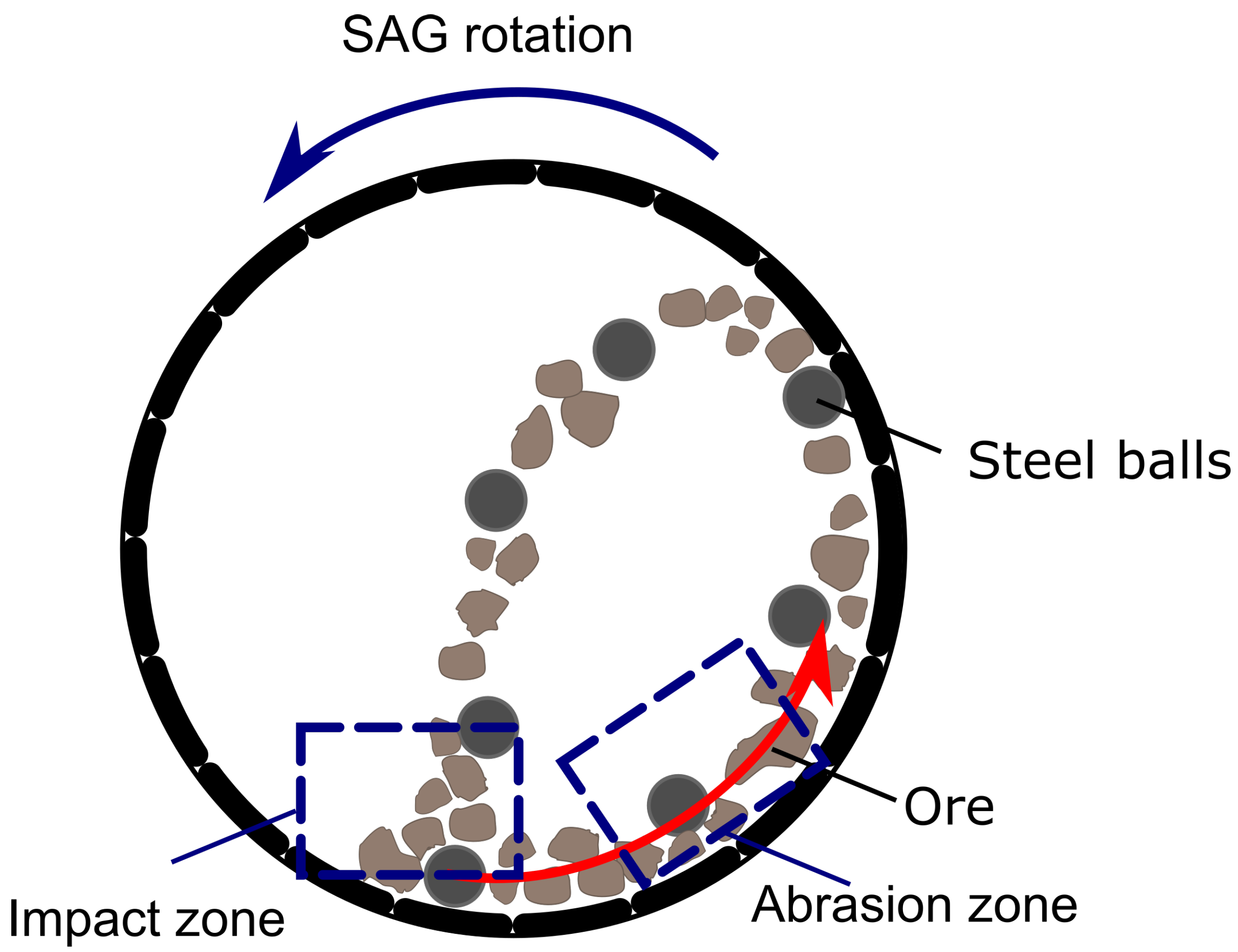
• Size reduction: it seeks to increase the liberation of valuable minerals from gangue minerals through the reduction in particle size. Part of this process is carried out in mills, in which water is added to the ore prior to its operation. This is where the operation of SAG mills is considered, as these devices play a crucial role in the reduction in ore size and the preparation of the material for the subsequent stages of the process.
• Classification: consists of separating the grinding product according to its size. Fine particles that meet the required size criteria are directed towards flotation, whereas larger coarse particles that exceed the specified size are sent back for regrinding.
• Concentration: achieved through processes such as flotation, involves enriching the ore by removing non-valuable components, generating a valuable ore concentrate.

As mentioned above, the SAG mill is one of the main elements in the size reduction process. The most relevant characteristic of SAG mill is the capacity to process ore, which supports its implementation despite the high associated energy cost. The operation of the mill is based on the fragmentation of the mineral through the abrasion and impact forces generated by the physical interaction between the grinding media (steel balls) and the mineral particles in the slurry (Figure 1).

Aside from parameters fixed at design (mill dimensions, installed power, and the circuit type), the major variables affecting the SAG mill circuit performance, according to [4] are related to: (1) ore hardness of the feed material, which plays a pivotal role in shaping the mill’s performance; (2) distribution of feed particle sizes, which significantly impacts the efficiency of the grinding process, and (3) the SAG mill operating variables, such as mill rotational speed, density, and total mill load.

3. Methodology

In this section, we describe the methodology utilized to comprehensively investigate and identify operational regions specific to the context of SAG mills. Our approach involves machine learning algorithms, including K-means clustering and self-organizing maps (SOMs), to discern patterns and relationships within the intricate operational landscape that defines these regions.

3.1. Dataset

For model development, a dataset containing data from 10 SAG operational variables is considered. These are described in

Table 1. Dataset variables.

Variable	Parameter	Unit
Timestamp	Sampling time	min
TPH total	Inbound material to the mill	TPH
SAG speed	Mill speed	RPM
Thick split	Coarse material percentage	TPH
Water	Inbound water to the mill	m${}^3$/h
SAG weight	Total mill weight	ton
Power SAG	Power consumed	kW
Size	Percentage solids F80	in
Rock hardness	Ore hardness	kWh/t
Pebbles	Recirculating pebbles	TPH

. The dataset considered an initial size of 50,700 instances with an associated sampling time of 5 min, extracted from a SAG mill located in a concentrator plant in northern Chile. This dataset collects the information on the SAG mill in operation from 1 January to 24 June 2020.

The dataset used in this study was collected from an AVEVA PI system data infrastructure. While the system provided the flexibility for smaller sampling times, a 5 min sampling interval was selected for this work. This choice was made based on the dynamic properties of the SAG mill and prior studies in the field of data-driven models for grinding. During the data preprocessing phase, we undertook several measures to enhance the quality of the dataset. Instances linked to maintenance periods and scheduled detentions were eliminated. Additionally, we identified and removed data points influenced by sensing errors. To address outliers, we applied a filtering criterion that excluded values lying beyond 2 standard deviations from the data mean; the specific choice of a threshold of 2 standard deviations was selected by the dynamic and variations in the SAG mill operational conditions (considering the fact that the study used data for a system under control, which is intended to reduce the variability of SAG mill operational variables). We decided to follow the standard deviation rule for identifying outliers, because, as has been proven, that works correctly for symmetric distributions, and the standard rule for this outlier detection method indicates that more than three standard deviations from the mean may be considered an outlier [24] but is also possible to find 2.5 or 2 standard deviations depending on the system. Subsequently, a correlation analysis was carried out to identify the most relevant variables, which was complemented with a phenomenological and empirical study of the SAG mill [25]. Finally, 41,095 samples and 7 variables remained from the initial dataset. These variables are: inbound material to the mill, SAG speed, water inside the mill, size of the ore, rock hardness (determined by SMC test), total weight, and energy consumed by the SAG mill.

3.2. Machine Learning Models

For model development, we used two clustering methods. The first one was K-means, which uses an unsupervised learning approach, where the objective is to find groups based on their characteristics. Then, we applied self-organizing maps (SOMs), which have the capability to group data of great similarity in a low-dimensional space, preserving the relationship between them. This allows us to watch the result in a two-dimensional plane, which can be useful in the visualization process at the control room.

3.2.1. K-Means

K-means seeks to find groups in the data. The algorithm can be described in three stages: (1) initialization, where k centroids are created, with one for each cluster. Each centroid is a point that inhabits the same space as the data and can be randomly created; (2) assignment, where dataset instances are assigned to the nearest centroid, creating preliminary clusters; and (3) update, where the position of each centroid is replaced by the average (of the values) of the previously assigned instances [26]. The assign-and-update steps are repeated until the centroids do not change, or the change occurs below a predefined threshold. The following equation describes this process.

$$d=\sum _{k=1}^K\sum _{i=1}^N{∥x_i-u_k∥}^2$$

(1)

where:

• d: total distance between data points;
• K: number of clustering centers;
• N: total number of data points in the dataset;
• $u_k$: k-th center;
• $x_i$: i-th point in dataset.

3.2.2. SOM

The self-organizing map (SOM) or Kohonen network is a neural network model that permits the visualization of high-dimensional data. It converts the nonlinear statistical relationships between high-dimensional data into simple geometric relationships of their points on a low-dimensional display (two-dimensional grid of nodes). SOM compresses information while preserving the most important topological or metric relationships in the data. Each unit in the map is equipped with a weight vector, where the number of elements is equal to the number of variables per input object [27]. The use of SOM allows not only for a clearer visualization of the operational regions for SAG mill operators, but it may also be helpful in the formulation of predictive controllers with set-valued constraints [22].

The elements of all weight vectors need to be initialized by values in a specific range in a dataset. Usually, for each map layer, the unit elements are initialized by a small random number added to the average value of the corresponding variable obtained for the entire training set. Then, individual objects belonging to the pre-selected training set are presented in random order to all units in the network. The unit in the map possessing the weight vector most similar to the presented object is assigned to be the winner. Subsequently, the weight vectors of this unit and its closest neighbors are updated by calculating the difference between the actual input object and the respective weight vector, and adding this difference dampened by some factor to the original weight vector. This iterative process of weight updating is repeated until all objects belonging to the training set are presented a sufficient number of times to the network [28].

3.2.3. Performance Metrics

Once the appropriate machine learning model is selected for a specific task, the next critical step involves evaluating its performance using relevant metrics. In our study, the application of two key metrics, namely inertia and silhouette score, playing a pivotal role in rigorously assessing the effectiveness of the clustering algorithms employed.

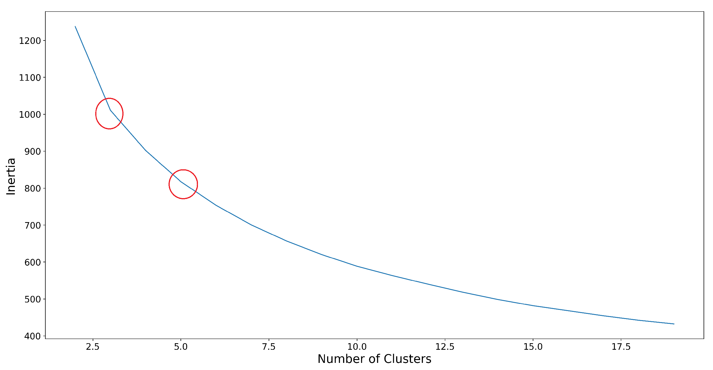
• Inertia: Is the square of the average distance between each instance (vector) and its nearest centroid. The smaller the inertia, the denser the cluster. However, it is also not advisable to consider the smallest inertia, as this would result in a poor model. That said, a middle point is considered, which is referred to as the ’elbow.’ The point where an elbow is observed indicates a good number of clusters for the dataset. As can be seen in Figure 2, two elbows are enclosed within a red circle, where you can observe how the curve changes its direction. This occurs with K equal to 3 and equal to 5, indicating that these would be good values for the number of clusters in our data.

  Figure 2. Inertia metric. Elbows are enclosed in red.

  Figure 2. Inertia metric. Elbows are enclosed in red.
• Silhouette score: this metric varies in the range of [−1, 1]. A score of 1 indicates that the instance is well within its own cluster and far from others; a value close to 0 suggests that the instance is near the perimeter of another cluster; and a value close to −1 means that the instance could have been assigned to the wrong cluster. In Figure 3, one can see how the values range between 0.35 and 0.1. From Figure 3, it can be observed that, with 2 or 5 clusters, the results show a variation of 0.15 in the Silhouette score.

  Figure 3. Silhouette score metric. Critical K values are enclosed in red.

  Figure 3. Silhouette score metric. Critical K values are enclosed in red.

After examining both the inertia and silhouette values in the dataset, it is determined that the tests will be conducted with two and three different clusters. This decision is based on the observation that, as shown in both metrics, having more than five clusters does not result in proper grouping. This is because the boundary of one cluster is very close to the perimeter of another cluster, which can create issues in determining whether a data point belongs to one group or another.

4. Results

This section presents the configurations used in the development of the models, as well as the performance obtained from the application of each of these.

4.1. K-Means

First, we conducted the test with two clusters (K = 2), and the results were analyzed as shown in

Table 2. K-means, K = 2.

Variable	Mean Val Cluster 0	Mean Val Cluster 1
TPH (TPH)	2588.2	2447.8
SAG speed (RPM)	9.16	9.51
Water (m${}^3$/h)	899.5	895.4
SAG weight (ton)	3853.5	3885.8
Power SAG (kW)	12,717.4	13,291.8
Size (in)	3.15	3.74
Rock hardness (kWh/t)	16.74	45.56

. In this table, we report the mean value of each parameter associated with both clusters (cluster 0 and cluster 1).

Then, we perform the test with three clusters (K = 3), and the resulting values are presented in

Table 3. K-Means, K = 3.

Variable	Mean Val Cluster 0	Mean Val Cluster 1	Mean Val Cluster 2
TPH (TPH)	2587.6	2395.3	2557.0
SAG speed (RPM)	9.11	9.53	9.37
Water (m${}^3$/h)	891.5	901.9	902.7
SAG weight (ton)	3851.3	3894.6	3865.8
Power SAG (kW)	12,704.9	13,405.7	12,931.7
Size (in)	3.51	3.86	3.55
Rock hardness (kWh/t)	12.07	52.04	31.79

. In this table, we also report the mean value of each parameter associated with cluster 0, cluster 1, and cluster 2.

4.2. SOM

Once K-means with two and three clusters has been applied, we apply SOM on these clusters with the goal of obtaining a two-dimensional plane.

The training performed to generate the model consisted of 1000 iterations. The initialization of the neuron values was defined randomly, in a map with dimensions of 20 × 20. For the calculation of the distance in each iteration, the Euclidean metric was used. First, we apply the SOM model in K = 2 (cluster 0 and cluster 1). In Figure 2, a clear grouping trend is identified for cluster 1 where its main grouping was the lower center of the map. In cluster 0, however, the data presented a greater tendency to group together and cover the upper area of the map.

Then, the SOM model was applied in the test with 3 clusters (cluster 0, cluster 1, and cluster 2). In Figure 4, the presence of a new cluster (Cluster 2) that grouped the data present in the limits of Figure 5 tended to mix in certain positions of the map. Therefore, cluster 2 segregates the previous clusters.

Based on these results, it is possible to identify different regions based on the different clusters. Table 2 and Table 3 present the mean values of these regions.

4.3. Sensitivity Analysis

For this final process, we considered the phenomenological and empirical study of the SAG mill, selecting the five variables that had more impact in the SAG mill as: TPH, water, power SAG, size and rock hardness [25]. This test was performed with three clusters, the main values of which can be seen in

Table 4. Sensitivity analysis, K = 3.

Variable	Mean Val Cluster 0	Mean Val Cluster 1	Mean Val Cluster 2
TPH (TPH)	2400.6	2553.1	2581.9
Water (m${}^3$/h)	899.6	900.6	888.3
Power SAG (kW)	13,365.9	12,919.0	12,679.4
Size (in)	3.85	3.54	3.5
Rock hardness (kWh/t)	51.8	31.49	12.00

.

We repeated the same process using SOM. Figure 6 shows the results of the analysis. It is possible to appreciate in this figure that the grouping is similar to the one shown in Figure 4. However, in the case of SOM, the colors and positions of the clusters are different. This happened because the algorithm initializes the weights randomly at the nodes. As in the previous figures, it is still possible to clearly identify the different areas identified by the cluster analysis.

5. Conclusions and Future Work

This study introduced the use of machine learning models tailored to the identification of distinct operational regions within SAG mills, focusing on ore type properties such as rock hardness and particle size. Additionally, we incorporated essential process variables, including tons per hour, water usage, and power consumption, to enhance the precision of our analysis.

Our findings reaffirmed the expected influence of rock hardness as the most significant factor in cluster creation. In addition, the noteworthy impact of TPH and particle size on the operational regions within the SAG mill was also shown as expected. The consistent results obtained from clustering with the application of two different unsupervised machine learning models validate that operational regions within the SAG mill operation can be effectively identified using data-driven methods. These results are suitable to be integrated into real-time mill control systems, thus providing control designers and operators with tools to optimize performance, that can lead to ensuring the necessary production rate, while achieving energy optimization.

Future work considers the implementation of a model predictive controller using the identified regions, and using a digital twin platform to further demonstrate the feasibility of our approach. Other future steps are associated with partnering with a mining company in order to implement these models within a model predictive control in a real mining setting.

References

1. Comision Chilena del Cobre. Proyección del Consumo de Energía Eléctrica en la Minería del Cobre 2019–2030; Technical Report; COCHILCO: Santiago, Chile, 2019.
2. Kawatra, S.K.; Young, C. SME Mineral Processing & Extractive Metallurgy Handbook; Society for Mining Metallurgy & Exploration (SME): Denver, CO, USA, 2019; p. 279. [Google Scholar]
3. Salazar, J.L.; Valdés-González, H.; Vyhmesiter, E.; Cubillos, F. Model predictive control of semiautogenous mills (sag). Miner. Eng. 2014, 64, 92–96. [Google Scholar] [CrossRef]
4. Sbárbaro, D.; del Villar, R. Advanced Control and Supervision of Mineral Processing Plants; Springer: London, UK, 2010. [Google Scholar] [CrossRef]
5. Owusu, K.B.; Skinner, W.; Asamoah, R. Feed hardness and acoustic emissions of autogenous/semi-autogenous (AG/SAG) mills. Miner. Eng. 2022, 187, 107781. [Google Scholar] [CrossRef]
6. Owusu, K.B.; Skinner, W.; Asamoah, R.K. Acoustic Sensing and Supervised Machine Learning for In Situ Classification of Semi-Autogenous (SAG) Mill Feed Size Fractions Using Different Feature Extraction Techniques. Powders 2023, 2, 299–322. [Google Scholar] [CrossRef]
7. Avalos, S.; Kracht, W.; Ortiz, J.M. An LSTM Approach for SAG Mill Operational Relative-Hardness Prediction. Minerals 2020, 10, 734. [Google Scholar] [CrossRef]
8. Acuña, G.; Curilem, M.; Cubillos, F. Development of a software sensor based on a narmax-support vector machine model for semiautogenous grinding. Rev. Iberoam. Automática Informática Ind. RIAI 2014, 11, 109–116. [Google Scholar] [CrossRef]
9. Olivier, J.; Aldrich, C. Dynamic Monitoring of Grinding Circuits by Use of Global Recurrence Plots and Convolutional Neural Networks. Minerals 2020, 10, 958. [Google Scholar] [CrossRef]
10. Liao, Z.; Xu, C.; Chen, W.; Chen, Q.; Wang, F.; She, J. Effective Throughput Optimization of SAG Milling Process Based on BPNN and Genetic Algorithm. In Proceedings of the 2023 IEEE 6th International Conference on Industrial Cyber-Physical Systems (ICPS), Wuhan, China, 8–11 May 2023; pp. 1–6. [Google Scholar] [CrossRef]
11. Hoseinian, F.S.; Aliakbar, A.; Bahram, R. Semi-autogenous mill power prediction by a hybrid neural genetic algorithm. J. Cent. South Univ. 2018, 25, 151–158. [Google Scholar] [CrossRef]
12. Avalos, S.; Kracht, W.; Ortiz, J.M. Machine Learning and Deep Learning Methods in Mining Operations: A Data-Driven SAG Mill Energy Consumption Prediction Application. Mining Metall. Explor. 2020, 37, 1197–1212. [Google Scholar] [CrossRef]
13. Hoseinian, F.S.; Faradonbeh, R.S.; Abdollahzadeh, A.; Rezai, B.; Soltani-Mohammadi, S. Semi-autogenous mill power model development using gene expression programming. Powder Technol. 2017, 308, 61–69. [Google Scholar] [CrossRef]
14. Kahraman, A.; Kantardzic, M.; Kahraman, M.M.; Kotan, M. A Data-Driven Multi-Regime Approach for Predicting Energy Consumption. Energies 2021, 14, 6763. [Google Scholar] [CrossRef]
15. López, P.; Reyes, I.; Risso, N.; Aguilera, C.; Campos, P.G.; Momayez, M.; Contreras, D. Assessing Machine Learning and Deep Learning-based approaches for SAG mill Energy consumption. In Proceedings of the 2021 IEEE CHILEAN Conference on Electrical, Electronics Engineering, Information and Communication Technologies (CHILECON), Valparaíso, Chile, 6–9 December 2021; pp. 1–6. [Google Scholar] [CrossRef]
16. Dorkhah, A.; Arab Solghar, A.; Rezaeizadeh, M. Experimental Analysis of Semi-autogenous Grinding Mill Characteristics under Different Working Conditions. Iran. J. Sci. Technol. Trans. Mech. Eng. 2020, 44, 1103–1114. [Google Scholar] [CrossRef]
17. Olivier, J.; Aldrich, C. Use of Decision Trees for the Development of Decision Support Systems for the Control of Grinding Circuits. Minerals 2021, 11, 595. [Google Scholar] [CrossRef]
18. Zhou, P.; Chai, T.; Sun, J. Intelligence-Based Supervisory Control for Optimal Operation of a DCS-Controlled Grinding System. IEEE Trans. Control. Syst. Technol. 2013, 21, 162–175. [Google Scholar] [CrossRef]
19. Saldaña, M.; Gálvez, E.; Navarra, A.; Toro, N.; Cisternas, L.A. Optimization of the SAG Grinding Process Using Statistical Analysis and Machine Learning: A Case Study of the Chilean Copper Mining Industry. Materials 2023, 16, 3220. [Google Scholar] [CrossRef] [PubMed]
20. Loudari, C.; Cherkaoui, M.; Bennani, R.; Harraki, I.E.; Younsi, Z.E.; Adnani, M.E.; Abdelwahed, E.H.; Benzakour, I.; Bourzeix, F.; Baina, K. Predicting energy consumption of grinding mills in mining industry: A review. AIP Conf. Proc. 2023, 2814, 040003. Available online: https://pubs.aip.org/aip/acp/article-pdf/doi/10.1063/5.0148768/18038672/040003_1_5.0148768.pdf (accessed on 10 August 2023).
21. Mayne, D.Q. Model predictive control: Recent developments and future promise. Automatica 2014, 50, 2967–2986. [Google Scholar] [CrossRef]
22. Risso, N.; Altin, B.; Sanfelice, R.G.; Sprinkle, J. Set-Valued Model Predictive Control. In Proceedings of the 2021 60th IEEE Conference on Decision and Control (CDC), Austin, TX, USA, 14–17 December 2021; pp. 283–288. [Google Scholar]
23. Raković, S.V.; Zhang, S.; Hao, Y.; Dai, L.; Xia, Y. Convex MPC for exclusion constraints. Automatica 2021, 127, 109502. [Google Scholar] [CrossRef]
24. Dunn, P.K. Scientific Research and Methodology: An Introduction to Quantitative Research in Science and Health; RStudio, PBC: Boston, MA, USA, 2021. [Google Scholar]
25. Wills, B.; Finch, J. Wills’ Mineral Processing Technology: An Introduction to the Practical Aspects of Ore Treatment and Mineral Recovery; Elsevier: Amsterdam, The Netherlands, 2015. [Google Scholar]
26. Jin, X.; Han, J. K-Means Clustering. In Encyclopedia of Machine Learning; Sammut, C., Webb, G.I., Eds.; Springer: Boston, MA, USA, 2010; pp. 563–564. [Google Scholar] [CrossRef]
27. Kohonen, T. Self-Organizing Maps; Springer Series in Information Sciences; Springer: Berlin, Germany, 1995; Volume 30. [Google Scholar] [CrossRef]
28. Melssen, W.; Wehrens, R.; Buydens, L. Supervised Kohonen networks for classification problems. Chemom. Intell. Lab. Syst. 2006, 83, 99–113. [Google Scholar] [CrossRef]
Figure 1. A section view of a SAG mill. Steel balls are shown in dark gray; the operation zone is shown in blue boxes.
Minerals 13 01360 g001
Figure 4. Results SOM K = 3.
Minerals 13 01360 g004
Figure 5. Results SOM K = 2.
Minerals 13 01360 g005
Figure 6. Sensitivity analysis result.
Minerals 13 01360 g006