A Natural GMS Laboratory (Granulometry-Morphometry-Situmetry): Geomorphological-Sedimentological-Mineralogical Terrain Analysis Linked to Coarse-Grained Siliciclastic Sediments at the Basement-Foreland Boundary (SE Germany)

Abstract

The “natural GMS laboratory” (granulometry-morphometry-situmetry) is located within the Variscan Basement in SE Germany (Fichtelgebirge Mts.), which is uplifted relative to its Permo-Mesozoic foreland along a deep-seated lineamentary fault zone. This transitional study area is crossed by straight to low drainage systems in the basement, turning meandering channel systems into high sinuosity when entering the foreland. Due to its good geological coverage, the entire region is subjected to an advanced-level terrain analysis and completed with a sedimentological study focusing on the GMS tool. Unlike many applications in the past, the three components of the GMS tool that are of almost equal value ought to be used in combination and not as stand-alone procedures so as to be integrated into other near-surface geoscientific methods, e.g., sediment petrography. The strong points of granulometry of coarse-grained/gravel-sized sediments are its extension into the smaller sand and clay grain size intervals using the sorting, mean and/or median values for an environmental analysis. Morphometry can be linked to the compositional geosciences, e.g., mineralogy and geochemistry. The grain shape is intimately connected with the lithology, providing options from triaxial measuring of the lithoclast to the digital image analysis. It is a favorable tool to supplement the provenance of lithoclasts. Situmetry is the key element of hydrodynamic research and directly builds upon its sister methods. Its applications and numerical approaches are useful for the identification and quantification of physical land-forming processes. It is the fan sharpness and the orientation of lithoclasts relative to the direction of the talweg and in relation cross-sectional valley features that integrate the GMS tool into geological and geomorphological mapping, both of which result in a digital terrain model. Horizontal rose diagrams are useful for the upper reaches of drainage systems, be they of alluvial or non-alluvial types, and vertical ones for alluvial channels in the distal and proximal foreland where stacked patterns of depositional terraces are of widespread occurrence. In general, the GMS tool can be applied to sedimentological, geomorphological, petrographic and tectonic objects in basements and foreland basins; in applied geosciences, it is suitable for the identification of mineral resources and of areas vulnerable to geohazards, and in genetic geosciences for the discrimination of supergene chemical and physical depositional and land-forming processes.

1. Introduction

One of the main goals of sedimentological geosciences is the study of depositional environments and the paleogeography of sedimentary basins at different scales. Not surprisingly, a lot of publications focusing on environment analysis are concerned with calcareous and siliciclastic sedimentary deposits alike, so that only a few comprehensive studies are given herein for reference to underpin the importance of this discipline [1,2,3,4,5,6,7,8,9,10].

Already during the 1930s, attempts were made to provide a numerical platform for terrigenous sediments based upon which of the environments of deposition can be categorized and interpreted by the aid of different granulometric discrimination diagrams [11,12,13,14,15,16,17,18,19]. More recently, published applications of the granulometric parameters revealed that these sedimentological methods may yield reasonable results for stratigraphic purposes, but no unequivocal ones for the analyses of the interpretation of the depositional environments as being used as a stand-alone method [20,21,22].

Another strategy to give insight into the environment is based on the grain shapes of the siliciclastic sediments, which are frequently expressed by the roundness and the sphericity of clasts [23,24]. The third method in this tripartite set of sedimentological methods measures the orientation of clasts and is called herein as “situmetry”. This method has been used as a stand-alone one in colluvial, fluvial and glacial deposits [25,26,27,28,29]. Unless the universal revolving table is used for oriented thin sections under the petrographic microscope, the third method is limited in its application to coarse-grain sizes detrital grains following the classical Udden–Wentworth particle scale for the GMS tool [30]: (1) gravel (>20 mm, cobble plus boulder), (2) sand (63 to 2000 µm, very fine- to very coarse-grained sand). Clay minerals are not considered for particle size in the current study for technical reasons.

The open questions debated in the current study and the issues awaiting clarification are as follows:

• How can the GMS triplet be subdivided, applied and linked up with other geoscience operatives under near-ambient conditions and in which theater of operation can each of them most favorably be used?
• How and where in applied and genetic geomorphology and sedimentology can the GMS tool successfully be used to tackle environment and provenance analyses?
• Which are the main goals of each element, granulometry, morphometry and situmetry, and how can they be achieved?
• To define new numerical parameters for each sub-tool to achieve the established goals on a field and laboratory scale.

In order to address these goals, a tripartite approach (GMS) was taken, and its results combined with those of a terrain analysis published under separate cover. The field work was devoted to the landscape hosting the terrigenous sediments, to determine the parameter to the best of one’s ability in an area which has been profoundly studied throughout the last decades [31,32,33,34,35,36,37,38,39,40,41,42]. This good coverage makes the Western Approaches of the Fichtelgebirge Mts., SE Germany, and its Permo-Mesozoic foreland an ideal place to set up what might be called “a natural sedimentological laboratory” (Figure 1 and Figure 2).

2. Methodology

The methods presented in this section are a selection to be used mainly in the field by geomorphologists and geologists alike, being in charge of mapping (“hammer-and-laptop strategy”).

2.1. Field Work

The focus of the current sedimentological-geomorphological study lies on the gravel size class with emphasis placed on the cobbles, small boulders and coarse pebbles [30,43,44]). During field work, a horizontal or vertical reference square measuring 1 × 1 m was outlined on the exposed clastic sediments. Between 50 and 150 gravel-sized lithoclasts were performed for situmetry, with about 200 hand specimens for granulometry and grain morphology [45,46]. It is the only way for measuring the clast orientation in the field using the strike or dip of the longest axis of the gravel-sized fragments at outcrop. The larger gravelly clasts are measured in the field using a digital caliper with regard to their grain size and their roundness has been determined based on visual inspection as compared to the reference charts of sensu [24]. For indoor morphological and granulometric studies, big-pack samples of the same number have been taken and the three axis of the clasts measured in the same way. The statistical treatment follows the suggestion put forward by [47]. As far as the sand samples are concerned, about 3 kg have been taken for follow-up granulometric and morphological measurements in the laboratory, applying the Camsizer technique.

2.2. Laboratory Work

Granulometric and morphological analyses: The granulometric and morphological field studies are extended into the laboratory where some sedimentological fine-tuning can be achieved. Sorting values and median are used as numerical parameters to characterize the granulometric variation of siliciclastic sediments [14,44,48,49]. The basic data are obtained from sieving and/or the CAMSIZER technique. The latter laboratory method is suitable for grain size and morphological analysis; likewise (sphericity), only in the interval <2000 µm, and as such only applicable when it comes to a comparison between gravel- and sand-sized grains.

Image analysis: The morphological parameters are measured by means of the ImageJ software using gravel photographs. Prior to this, the images were processed by means of Adobe Photoshop CS3 software (Apache Software Foundation, Wilmington, DE, U.S.A.). This process includes conversion to greyscale mode and adjusting contrast, levels and curves for a better contrasting view between the grains and background, without modifying the edges of each individual grain. The processed images are imported into the ImageJ software where most of the grains are selected automatically. Only those that share even point contacts edges are selected and the contours are handled manually. The following shape parameters are obtained: area, Feret diameter, circularity, aspect ratio, roundness and solidity. The area (size), circularity (sphericity) and roundness (angularity) have shown to be the most efficacious parameters and are mainly used in the subsequent sections.

2.3. Mineralogy and Petrology

Mineralogical and petrographic investigation are not the centerpieces of the current paper but saved for a different one, needed to some extent so as to determine the genetic relation between textural parameters and composition.

Petrographic microscopy: Routine thin section analysis was carried out in combination with optical microscopy (Zeiss microscope, Jena, Germany) of heavy and light minerals with 200 to 300 g counted per sample. Heavy mineral separation was performed for each sample to the grain size fractions richest in heavy minerals (the 3–4 fraction), using sodium polytungstate at a density of 2.9 g/cm³ [50].

Raman spectroscopy: The micro-Raman spectra were acquired by using the Renishaw InVia Raman Microscope system equipped with two laser sources with wavelengths of 532 nm and 785 nm and full power of 500 mW, with a CCD detector. The measurements were performed with the 532 nm wavelength laser with the 1800 L/mm holographic grid, at a power of 10%, exposure time of 1–5 s, and 10–20 acquisitions, using the zoom objective 50× from the Leica microscope attached to the spectrometer. The interpretation of the micro-Raman spectra was conducted using the LabSpec software by means of baseline correction and peak-fitting. It is the most advanced level and used for fine-tuning of the mineralogical results.

Electron microscopy: Scanning-electron analyses (SEM-EDX) are conducted by means of a QUANTA 600 FEG equipped with a GEMINI EDX system. Because all analyses were carried out under low-vac-chamber conditions (1 to 10 mbar), no sputter coater was used prior to analysis. It is run in combination with the XRD analysis.

X-ray analysis: X-ray diffraction (XRD) patterns are a supplement to the aforementioned method and were recorded using a Philips X´Pert PW3710 Θ-2Θ diffractometer (Cu-Kα radiation generated at 40 kV and 40 mA, equipped with a 1° divergence slit, a secondary monochromator, a point detector and a sample changer (sample diameter 28 mm). The samples were investigated from 2° to 80° 2Θ with a step size of 0.02° 2Θ and a measuring time of 3 sec per step. For specimen preparation the top loading technique was used.

2.4. Geochemistry

Major and trace elements were analyzed by X-ray fluorescence spectrometry. Powdered samples were analyzed using a PANalytical Axios and a PW2400 spectrometer. Samples were prepared by mixing with a flux material and melting into glass beads. The beads were analyzed by wavelength dispersive X-ray fluorescence spectrometry (WD-XRF). To determine loss on ignition (LOI), 1000 mg of sample material were heated to 1030 °C for 10 min. After mixing the residue with 5.0 g lithium metaborate and 25 mg lithium bromide, it was fused at 1200 °C for 20 min. The calibrations were validated by analysis of Reference Materials. “Monitor” samples and 130 certified reference materials (CRM) were used for the correction procedures.

2.5. Geomorphology

The geomorphometric analyses delivering numerical data for the slope angle, elevations and gradient have been used in previous studies and described by [41,42]. They were only adjusted to the current topic and modified to a larger scale. The database of the slope angle measurements was created based on field measurements measuring the inclination in some places and topographic maps on the scale of 1:25,000 with a resolution of a 5-m spacing in height of the contour lines. The determination of the slope angles was calculated for the same XYZ data by using Surfer’s Terrain Slope Calculus gridding function.

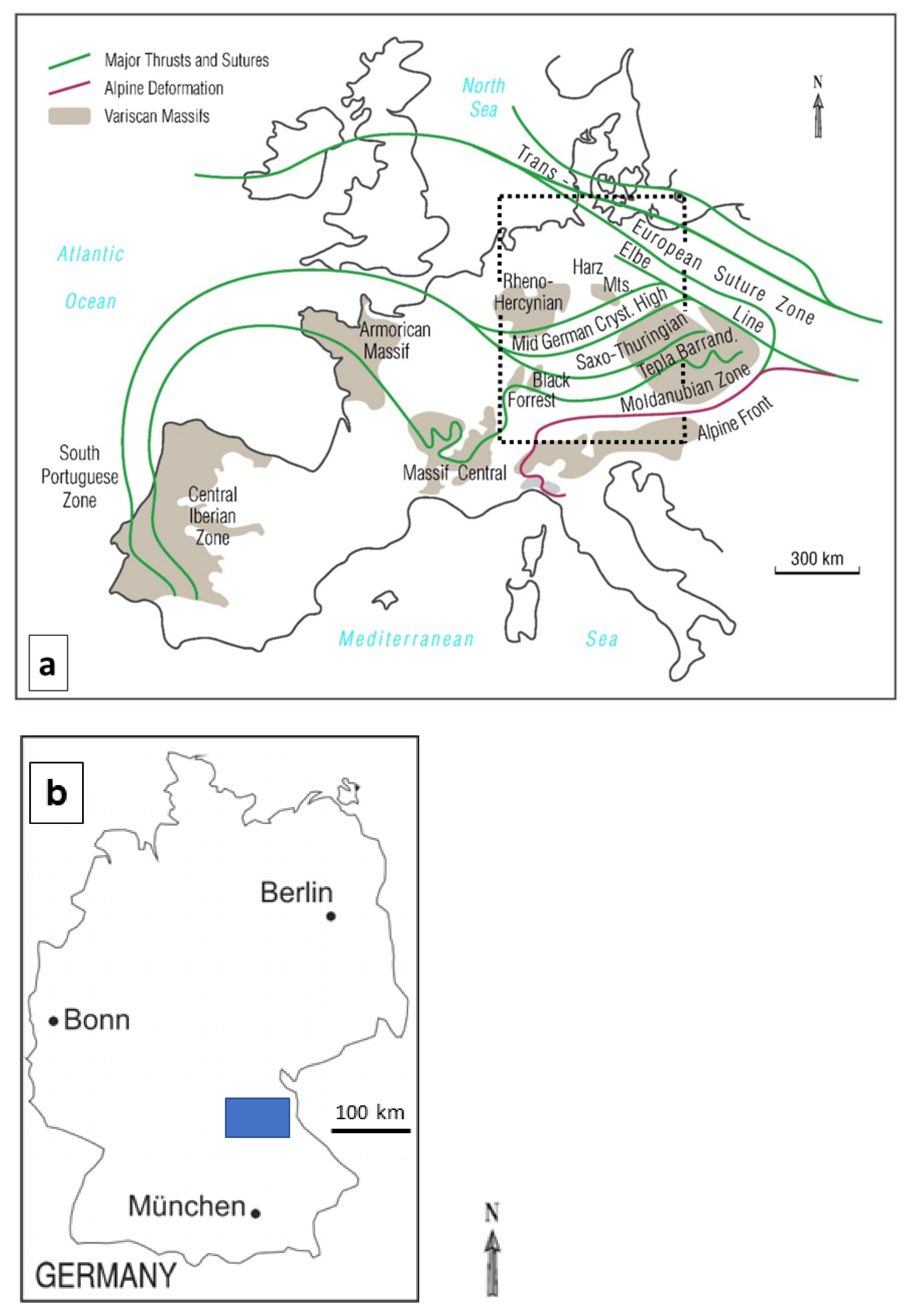
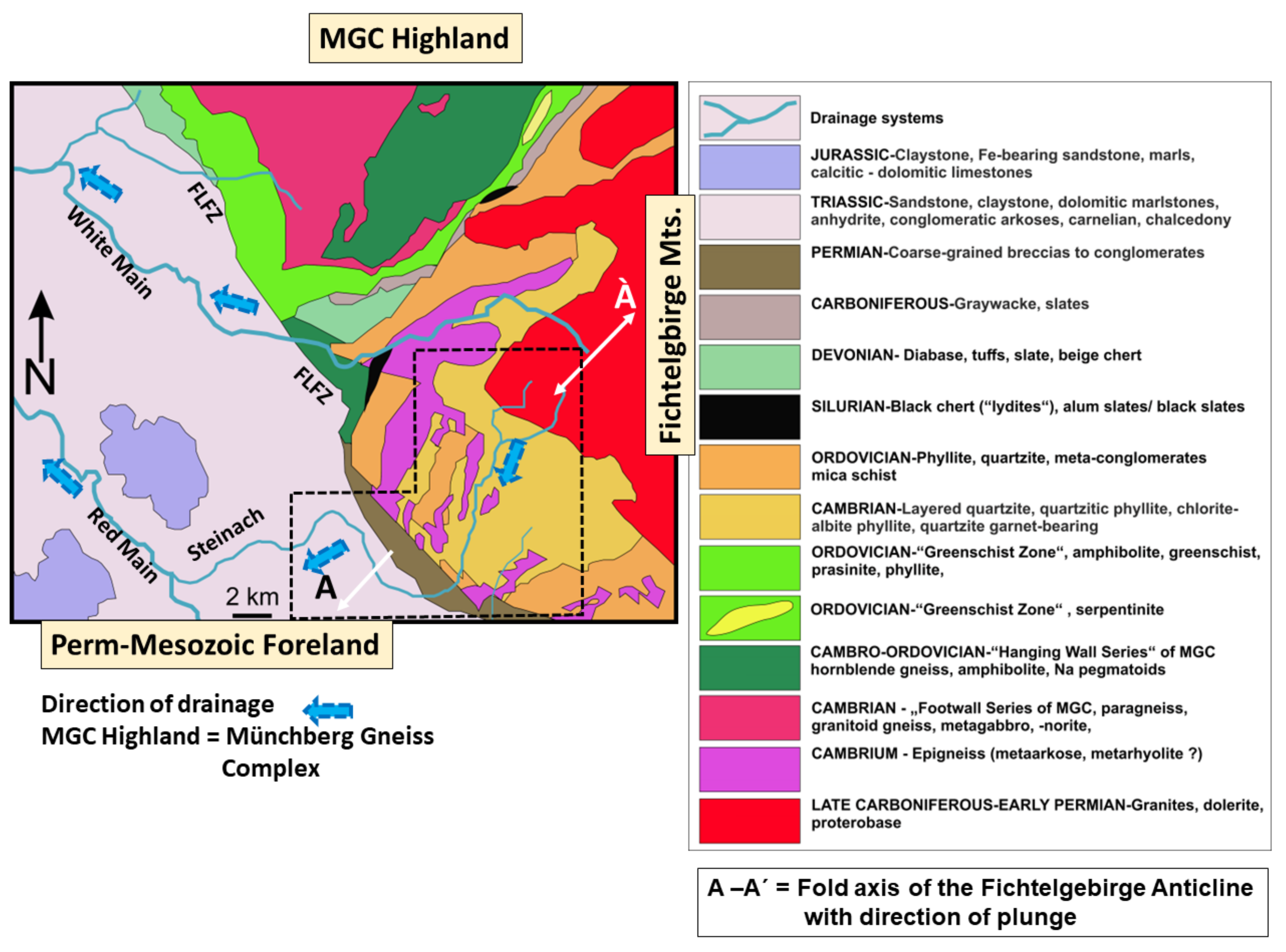
3. Geological Setting

The upper reaches of the Main and Steinach river systems run through a transition zone between basement rocks, represented by the Fichtelgebirge Mts. and by the Münchberg Gneiss Complex (MGC) Highlands in the NE and the Permo-Mesozoic foreland in the SW, both of which are located in SE Germany (Figure 2). The basement belongs to the Saxothuringian Zone, a geodynamic realm of the central European Variscides, which subsided during the Cambro–Ordovician as a rift basin NW of the Moldanubian Zone [51]. The MGC is an allochthonous lithological unit that was pushed towards the NW over the Fichtelgebirge and emplaced by thrustal nappe movements in its present position. In the MGC sensu stricto, we are faced with an allochthonous synform with a dual litho-stratigraphic subdivision into the so-called “Liegend-Serie” (footwall series) and the “Hangend-Serie” (hanging-wall series) of Cambrian to Ordovician metamorphic rocks (Figure 2). The aforementioned MGC is rimmed by a tripartite marginal series made up of the “Randschiefer-Series” (rim slate), “Phyllit-Prasinit-Series” (phyllite-prasinite), and the “Rand-Amphibolit” (rim amphibolite) denominated as the “Greenschist Zone” (Figure 2). The Early Paleozoic country rocks of the Fichtelgebirge Mts. are similar in age but geodynamically completely different due to their autochthonous position and lower metamorphic grade (Figure 3a,b). These meta-psammopelites were intruded during the Late Carboniferous and the Early Permian by granites, among them the G2 (marginal granite) and the G3 (core granite), which are largely exposed by the headward erosion of the Main and Steinach rivers (Figure 3). After the Variscan deformation, the entire basement complex became dryland and was uplifted along the deep-seated Franconian Line lineamentary fault zone [52] (Figure 2 and Figure 3a,b). It gave rise to the Permo-Mesozoic foreland, which is made up of Permian to Late Jurassic sediments, mainly siliciclastic in composition. Only during the Middle Triassic, “Muschelkalk”, a marine invasion, took place in the study area (Figure 2 and Figure 3). Sediments mainly of Triassic age constitute the basis of the depositional area of the Steinach River and the bedrock of the meandering drainage systems discussed in the precursor study [41,42]. Proximal to the basement bilateral symmetrically, coarse-grained red bed fanglomerates extend towards the NW and SE of Fichtelgebirge Anticline, the fold axis of which plunges towards the SW (Figure 2). Quaternary sediments were deposited during the evolution of the Steinach drainage system. They form the centerpiece of the present sedimentological study (Section 4) and are discussed in Section 5, with emphasis placed upon the gravel-sized sediments.

4. Results

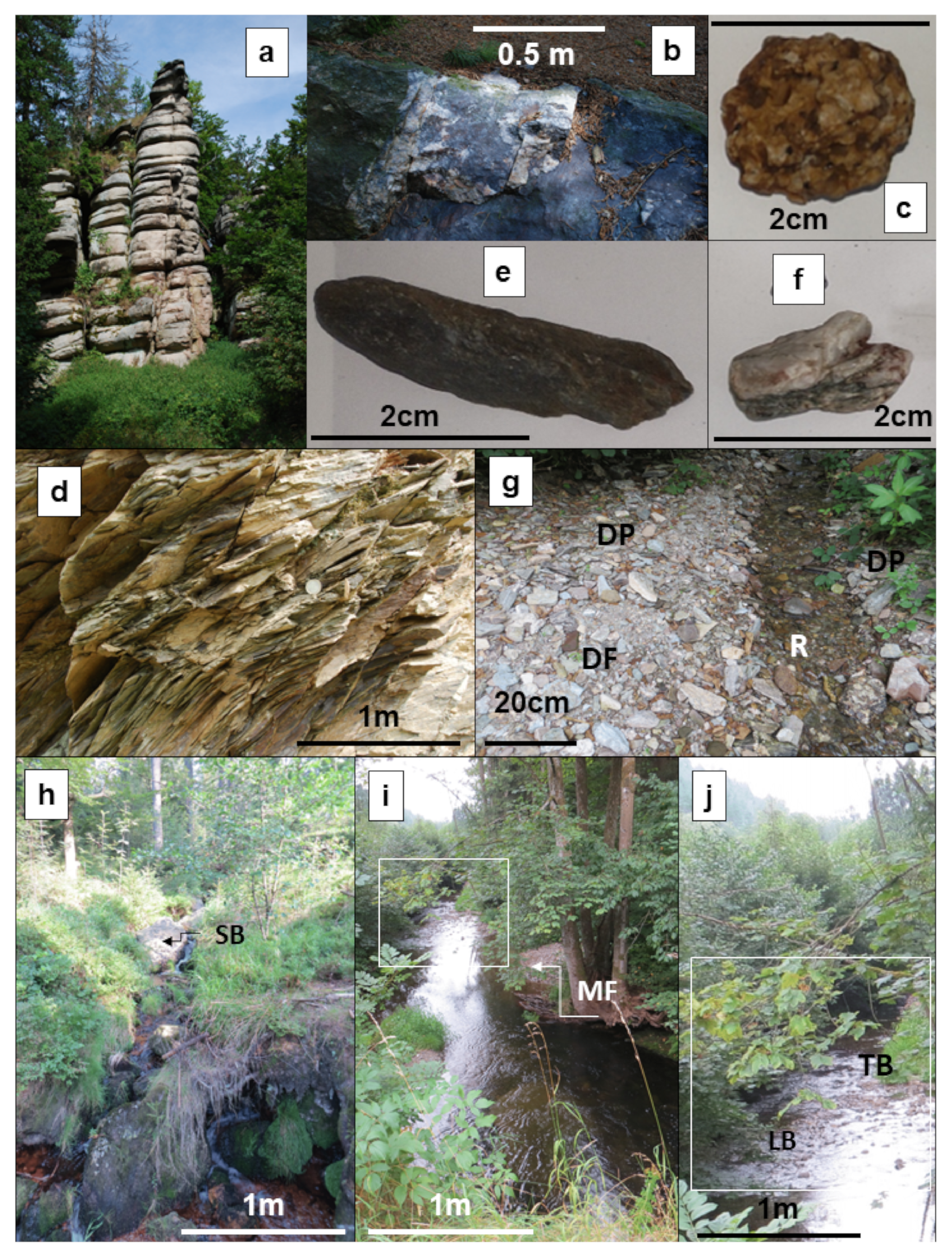
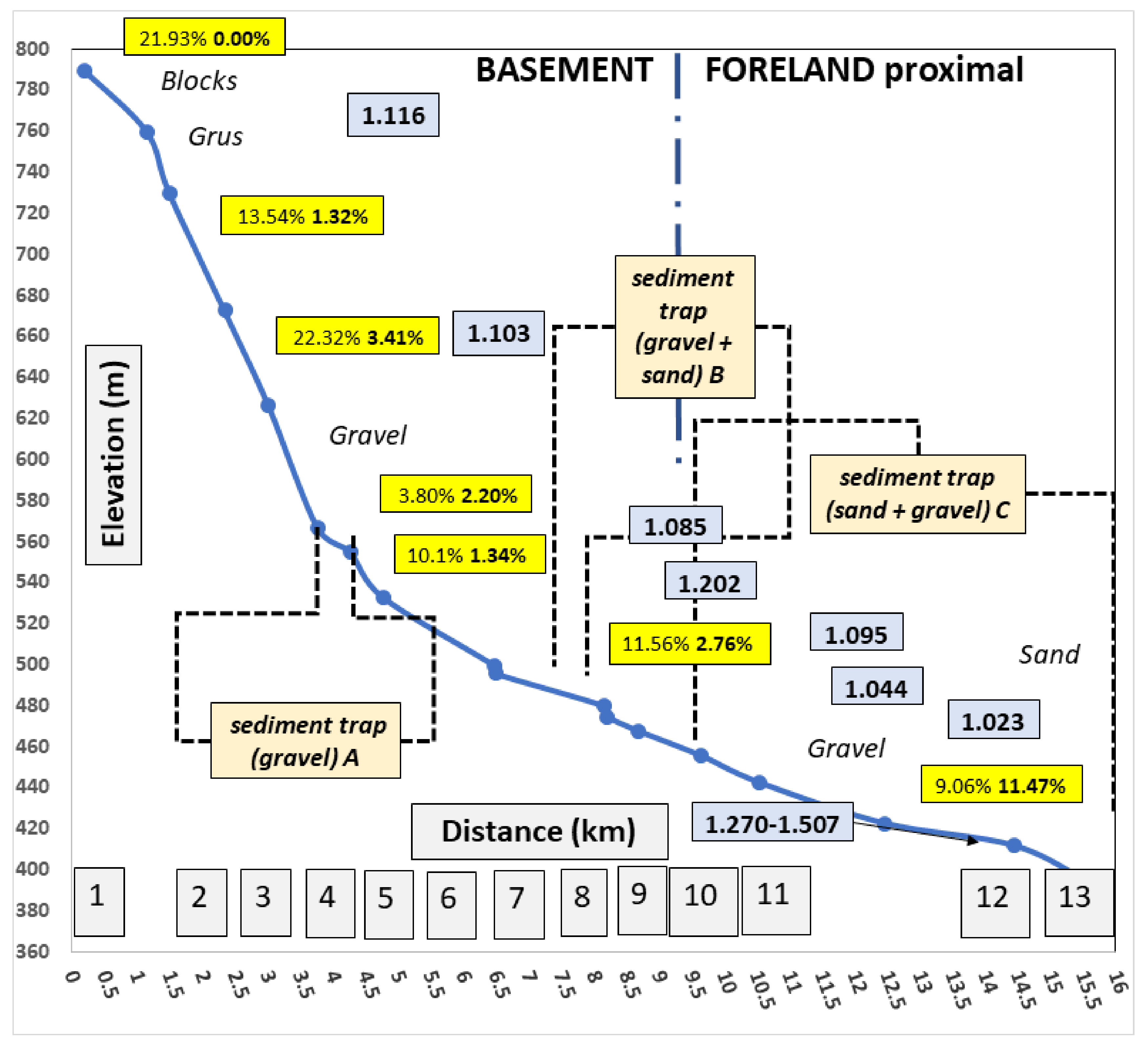
4.1. Geomorphology of the Steinach Drainage System

The current sedimentological study forms part of a tripartite approach taken during terrain analysis of a basement-foreland terrain. The geomorphological part has already been published and only some amendments have been performed during the current sedimentological study which are provided in the succeeding paragraphs of Section 4.1 to help understand the issues presented [41,42,53]). The amendments mainly concern a more detailed mapping of the country rocks of the Steinach drainage system, the results of which are illustrated in the map of Figure 3 and form the basis for the follow-up sedimentological studies. The landform series are depicted in Figure 4 and the numerical parameters of the drainage system plotted along a longitudinal profile in Figure 5. This set of figures acts as the platform for the “natural sedimentological laboratory”. A third study concerning the compositional data of this terrain analysis, based on sediment petrography/mineralogy and geochemistry, is in the making.

The description of the river course and the categorization of its three main sections, headwaters, zones of transport and deposition, are performed according to the proposals put forward by Knight et al. [54], Rodriguez and Garcia [55], Reineck and Singh [9] and Scheffers et al. [56].

The Steinach is made to arise on the upper slopes of the Ochsenkopf Summit, developing a dendritic alluvial channel system so as to be denominated as the zone of headwaters. Upslope of site 1, the summits of the Fichtelgebirge Mts. are topped by typical landform series belonging to the monadnocks. Mass wasting exhumed the syeno- and monzo-granites and, after having completely deprived them from their regolith, rendered the well-known tors to stand out from an ancient peneplain [57,58] (Figure 4a). The characteristic towers of woolsacks on the Fichtelgebirge summits display subhorizontal onion-shell fractures or sheet joints and subvertical mural joints originating from the cooling history of the granitic magma [59]. They take effect on the size and morphology of the granitic rock slabs as the granitic rocks disintegrate and show up in the bedload of the fluvial channels (Figure 3). The same also holds true for the quartz veins intersecting the granites which, in places, abundant in platy lustrous hematite, are accumulated along joints and fissures with a decimeter-spacing, in contrast to the jointing of their host granites that measure by the meter (Figure 4a,b). Dislodged blocks and bolder strewn elevation give rise to blockmeers. Scattered boulders may drift away from their source area on a thick “lubricant” layer of grus sensu [60]), into V-shaped valleys. These bolder-sized rocks are common to the upper reaches of the Steinach River and mark the transition from the headwaters into the zone of transport (Figure 4c,d).

This is a widespread phenomenon that appears at cataracts and occurs around the knickpoint at 760 m in the Steinach drainage system as a result of a fault tectonic, where the gradient significantly increases before entering into the intermediate sediment trap A of the “Warmensteinach Bowl” (Figure 5) [61,62]. It is the most elevated sediment trap filled up only with gravel. The downstream intermediate sediment traps B and C are both also enriched in sand. In the “Weidenberg Bowl” the flood plains are arranged in a quadripartite set of abandoned floodplains which are dissected by the Holocene drainage system of the Steinach (Figure 3 and Figure 5).

By and large, the mass wasting processes of the incipient phases of transport in the Steinach drainage system are mainly talus and soil creep, block sliding, topple and rockfall, the deposits of which were reworked and incised by confined flow processes (Figure 4g–j).

The passage into the transport zone is not only marked by a striking change in the land-forming processes but also by the appearance of a new suite of metapelitic bedrocks (Figure 4d). Tightly folded phyllitic slates, phyllites and quartzites are exposed on both banks of the Steinach River, in places, endowed with rod-like placoids sensu [63], made up of sandy material. The dendritic channel pattern converts into a long river course characterized by a non-alluvial single-channel system that has to be denominated as a strike stream system running subparallel to the strike of the metamorphic host rocks (sub) parallel to the south-westerly plunging fold axis of the Fichtelgebirge Anticline (Figure 2). The channel system features step-and-pool-dominated channels in the upper and middle valley sections, while changing into wandering low sinuosity channels with small longitudinal, and near the highland boundary fault also traverse gravel bars. The latter fluvial landforms subsequently grade into meandering river sections in their lower reaches of the Steinach, following the schematic classification schemes proposed by Nanson and Knighton [64], Church [65], Beechie et al. [66] and Charlton [67] (Figure 4i,j). The sinuosity given in the present study is calculated according to the suggestions put forward by Ahnert [68]. The sinuosity of the channels, the ratio of mass wasting vs. fluvial deposits along the river, and its gradient can be deduced from Figure 5 while forming the platform for the sedimentological follow-up analyses. At the basement-foreland boundary the river course suffers a relapse into an alluvial channel system with several active, abandoned flood plains arranged in a stacked pattern of terraces on the low scarp of the valley (Figure 3a,b).

There are also several small tributaries delivering from both sides coarse-grained material into the Steinach River and thereby contributing to the variegated lithology of the fluvial deposits. Not all of them are of the same fluvial type as the trunk river, as demonstrated by the deltaic fan at site 9 (Figure 4g). A discrete delta plain can be mapped and distinguished from a delta front prograding into the Steinach where it builds up a lobe in a relatively deep channel section (Figure 4i). Downstream of its entrance where the channel depth becomes shallower, a shoal of longitudinal and transverse bar sets develop from the reworking of the material put into the Steinach at site 8 (Figure 4j).

4.2. Lithology of the Gravel-Sized Fluvial and Colluvial Deposits

The variegated lithology of the fluvial and colluvial debris in and around the Steinach drainage system has to be split into two principal groups for grain-size reasons, because the GMS tool can successfully only be applied to gravel and, hence, debris of sand-sized material have to be excluded from being considered in the current sedimentological study but they are mentioned in

Table 1. Lithology of the detrital clasts of the Steinach-Main drainage system as a function of the distance to source and grain size. Normal font = occurs in the gravel-size class, italics = occurs only in the sand-size class. For the 10 km and 20 km zones, see Figure 3, and for the 50 km zone, Figure 2, as far as the potential source rocks are concerned.

	Basement < 10 km	Foreland < 20 km	Foreland < 50 km	Origin and Occurrence
Limestone				Triassic sulfate-bearing calcareous rocks of the “Weidenberg Bowl”
Carbonate gangue				Carbonate-bearing vein-type deposits
Fe mineralization				Supergene alteration, fluctuating ground water table
Ba-F ore mineralization				Barite-ankerite/siderite vein-type deposits -upstream of site 5 to site 10
Quartz aggregates				Granites, metapsammites, vein-quartz with/without hematite
Chert (black “lydite”)				Silurian to Early Devonian marine biogenetic sediments (low to non-metamorphic)
Silcrete, “carnelian				Early Triassic paleosols
Quartzite				Low grade metamorphic sandstones-metapelites of the country rocks of the Late Paleozoic granites
Sandston–conglomerate				Permian-Lower Triassic red beds foreland basin
Graywacke				Impure sandstone of Early Paleozoic age (low to non-metamorphic)
Phyllite				Low grade metamorphic claystones-metapelites of the country rocks of the Late Paleozoic granites
Mica schist				Phyllites of slightly higher metamorphic grade (contact metamorphic)
Granite				Late Paleozoic granites of the Fichtelgebirge domal anticline
Rhyolite-dacite				Early Permian volcanic rocks at the basement-foreland boundary
Epigneiss				Early Paleozoic low grade metamorphic meta-rhyolites or meta-arkoses
Lamprophyre-Proterobase				Basic dykes intersecting the granitic domes
Diabase				Early Paleozoic meta-basalts and metabasalt tuffs
Metavolcanic rocks				Hydrothermally altered volcanic rock manly of basic composition
Epidote-chlorite amphibolite				Low-grade basic volcanics and pyroclastic rocks-Ordovician Greenschist Zone
Serpentinite				Low-grade ultrabasic volcanics and pyroclastic rocks-Ordovician Greenschist Zone
Amphibolite				Basic volcanic rocks (medium-high grade) Ordovician Greenschist Zone, MGC Hanging Wall rocks
Mica gneiss (+ garnet)				Meta-psammopelites (medium-high grade) MGC Footwall rocks
Slags (Fe, Cu.) and processing artifacts				Historic Fe smelting and waste from ceramic industry (glass)

for the sake of completeness and comparison. These sand-sized lithoclasts are highlighted in Table 1 by italics while being mentioned in each of the eight lithofacies types.

The fine-grained calcareous rocks are composed almost completely of calcite and dolomite. They have been sourced from the distal Triassic foreland sedimentary units, called “Muschelkalk” and undergo rapid dissolution and disintegration in parts accelerated by the presence of gypsum and anhydrite which was locally mined in the region [69,70]. Limestone gravel appear only in site 13. This is also true for calcitic coarse-grained aggregates where the perfect cleavage of the carbonate crystals matters more than in the marine limestone. They have been derived from vein-calcite and are confined to sampling sites 8 and 9 [71].

Baryte associated with fluorite and Fe carbonates was concentrated in veins which are truncated by the Steinach channel [71]. The fragments eroded from the veins by the running water rapidly pass from the gravel into the sand-sized clasts spectrum and thereby escape the grain-size range appropriate for the GMS analysis. Gravel-sized “limonitic” fragments are observed within the Holocene channels cutting into basement rocks and rarely in terraces of the foreland [72,73]. They are rather friable and disappear very rapidly from the gravel-sized clasts into the sand fraction so that they can only be found within the range of a few kilometers between sites 8 and 12 and in some terraces of the “Weidenberg Bowl”.

Quartz aggregates are defined in the current study as a monomineralic intergrowth of at least two quartz grains. It may be monochrome or take on different colors from white to brown and red or to greenish shades caused by Fe oxides and chlorite, respectively, but present only as accessory minerals. These green aggregates have been derived from meta-psammopelites. They are preserved from attrition in notches of the siliceous aggregates so that they can be traced back to their meta-psammopelitic source rocks in the Fichtelgebirge Mts., even after more than a 100 km distance to source. Some quartz aggregates originating from vein-type mineralizations have their interstices filled with platy hematite attesting to hematite-bearing quartz veins which are quite common to the Fichtelgebirge–Erzgebirge Anticline, e.g., Gleißinger Fels [74,75] (Figure 4b). These fragments allow, owing to their ore minerals, to be identified with the naked eye. They occur only a few kilometers downstream of the site where the parent mineral veins are crossed by the river run.

Chemical siliceous sediments pertain to two different groups. It is the silicious marine biota, such as radiolarians, together with organic matter, make up the chert or black “lydite” and the paleosols and duricrusts called duricrusts or silcretes [76,77,78,79,80]. Owing to their rock strength and conspicuous black and red rock colors these siliceous rocks can act as a valuable provenance markers.

Psammopelitic sediments, such as phyllites, quartzites, and mica schists, are widespread in the wall rocks of the granites as low-grade metamorphosed quartzites and quartz phyllites that show up in the basement [81]. In the current study the BGS classification scheme of meta-psammopelitic lithologies was adopted, containing quartz, ±feldspar, ±mica, and < than 10% carbonate minerals [82]. A rising quantity of argillaceous matter renders these meta-psammitic rocks to grade into meta-pelitic rocks. The various meta-sedimentary rock types may be classified in the field and distinguished from each other according to their quartz (qtz) contents: qtz > 90 % quartzite (in places with layered phyllite intercalations), qtz 89 to 50% phyllitic quartzite, qtz 49 to 10 % quartzitic phyllite, qtz < 10% phyllite. For the current publication the end members quartzite and phyllite have proven to be sufficient to meet with the project scope.

In the foreland country rocks of the Steinach drainage system the non-metamorphosed sandstones, arkoses and conglomerates formed during the Early Triassic in the “Bunter Series”. The non-metamorphic psammites or sandstones are denominated as feldspar or lithic arenites dependent upon the predominance of feldspar over lithoclasts or vice versa [44]. The matrix of the Triassic sandstones and conglomerates is made up of illite and kaolinite. The ensuing decrease in rock strength along with an increase in clay minerals reduces the preservation potential of the Mesozoic arenite samples tremendously and impedes their appearance in the fluvial channels over a long distance. The term graywacke is confined to the impure basement sandstones which, due to their very-low to low-grade regional metamorphism, attain a higher rock strength and enables them to stand out among the gravel assemblage in the fluvial channels (Table 1),

Three different types of felsic magmatic rocks can be observed among the gravel association of the Steinach drainage system: (1) granites, (2) felsic to intermediate volcanic rocks, and (3) low-grade metamorphic rock named “epigneiss” (Table 1). All of them have been derived from different geodynamic realms and arranged in the following paragraphs according to the increasing resistance to mechanical and chemical destruction on transport (Table 1, Figure 2 and Figure 3). The monzo- and syeno-granitic specimens can easily be differentiated based upon their textural features. Coarse-grained to pegmatitic granites represented by the granite G3 (core granite) more rapidly disintegrate into smaller grus clasts than their fine-grained porphyritic equivalents called granite G2 (marginal granite). In the rivers granitic rocks disappear very rapidly after 2 to 5 km from their source under the harsh fluvial attrition in the non-alluvial watercourses of the basement.

Rhyolite and dacite have a higher preservation potential than the felsic intrusive rocks. Their bimodal grain size distribution of matrix and phenocrysts places these lithologies at an advantage to chemically equivalent granites and granodiorites in terms of weathering resistance and vulnerability to attrition. They are rare constituents but nevertheless a valuable tool and point to Permo- (Late) Carboniferous source rocks in the study region (Table 1).

Regional geologists used the term epigneiss for feldspar-muscovite gneisses which by international definition is an orthogneiss (meta-rhyolite) or paragneiss (meta-arkose) [33,35,82]. The metamorphic counterpart of granite and rhyolite has a higher preservation potential due to its preferred alignment of their rock-forming minerals and thermal overprinting.

Basic and ultrabasic rocks among the gravel assemblage can be distinguished based upon their texture, composition and geodynamic position following the classification scheme of Robertson [82]. This igneous suite encompasses meta-basaltic massive, porphyritic volcanic rocks and coarse-to-medium-grained specimens originating from dikes (dolerite, proterobase). Where hydrothermal alteration, such as splitisation or argillitization, was too intensive so as to enable us any precise identification of the rock-forming minerals and a determination of the parent material, the general term metavolcanic rocks is used for classification [83]. Serpentinites and epidote amphibolites (greenstones) belong to the Ordovician Greenschist Zone (Table 1, Figure 2).

Medium to high-grade metamorphic rocks, such as amphibolites and gneisses with and without garnet, originated from the denudation of metamorphic rock of the “Hanging Wall” and “Footwall” units of the MGC. They appear only in the 50-km foreland zone of the drainage system under consideration (Table 1, Figure 2).

Artifacts need to be mentioned in the debris assemblage of the creeks and rivulets for completeness. They are slags of ancient iron smelting [84]. They closely resemble in their outward appearance the limonitic ferricretes mentioned above (Table 1).

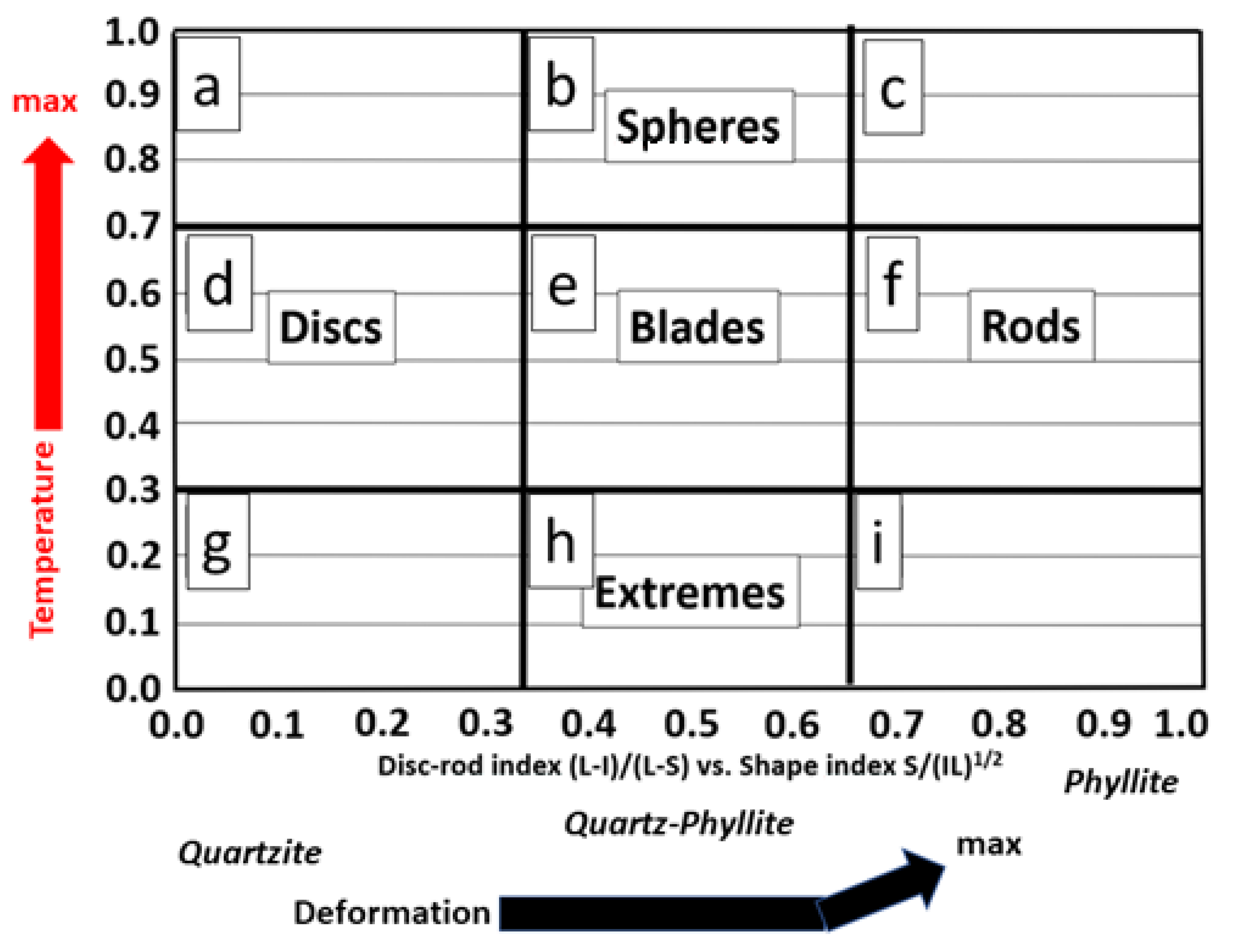
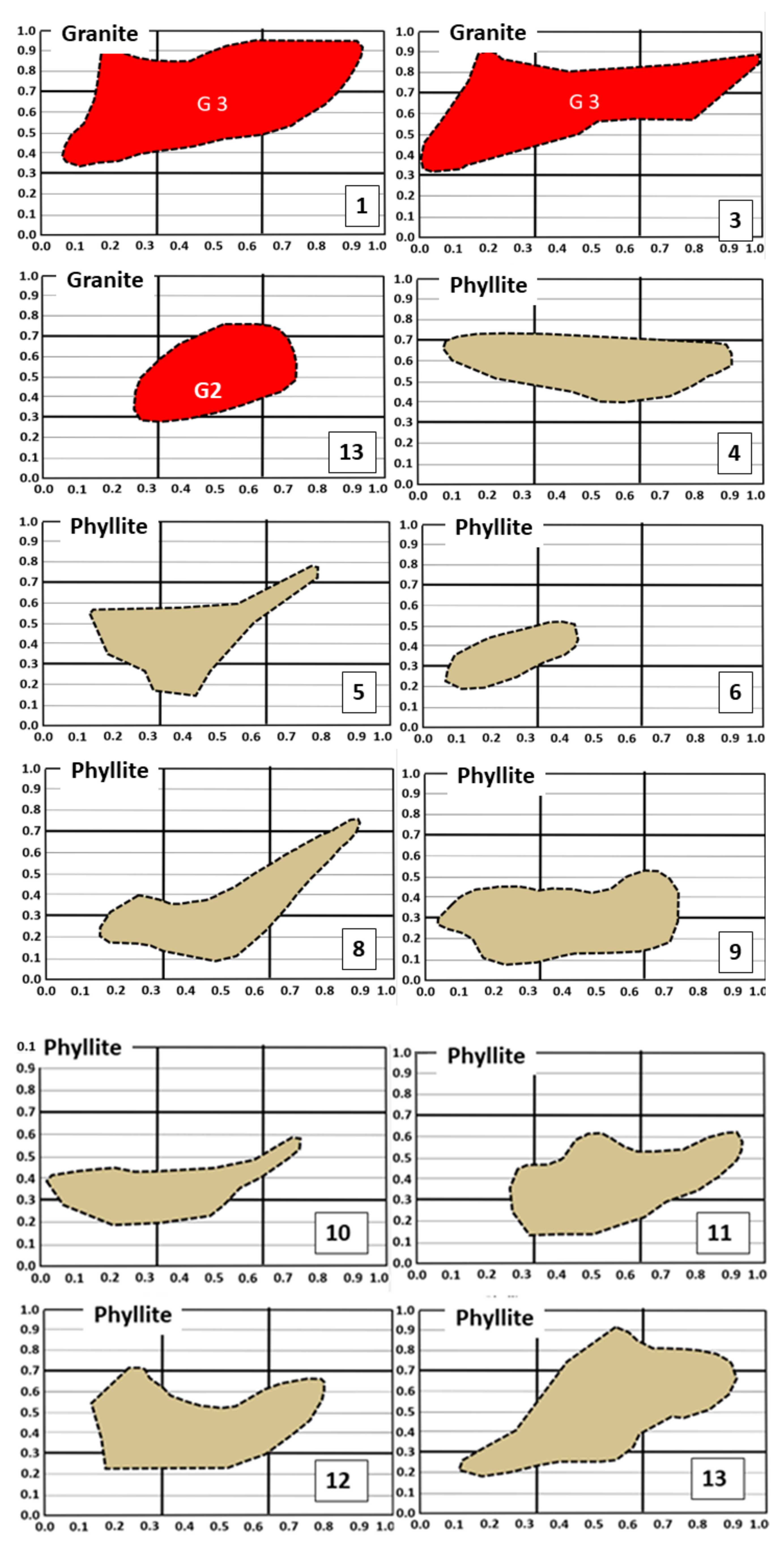
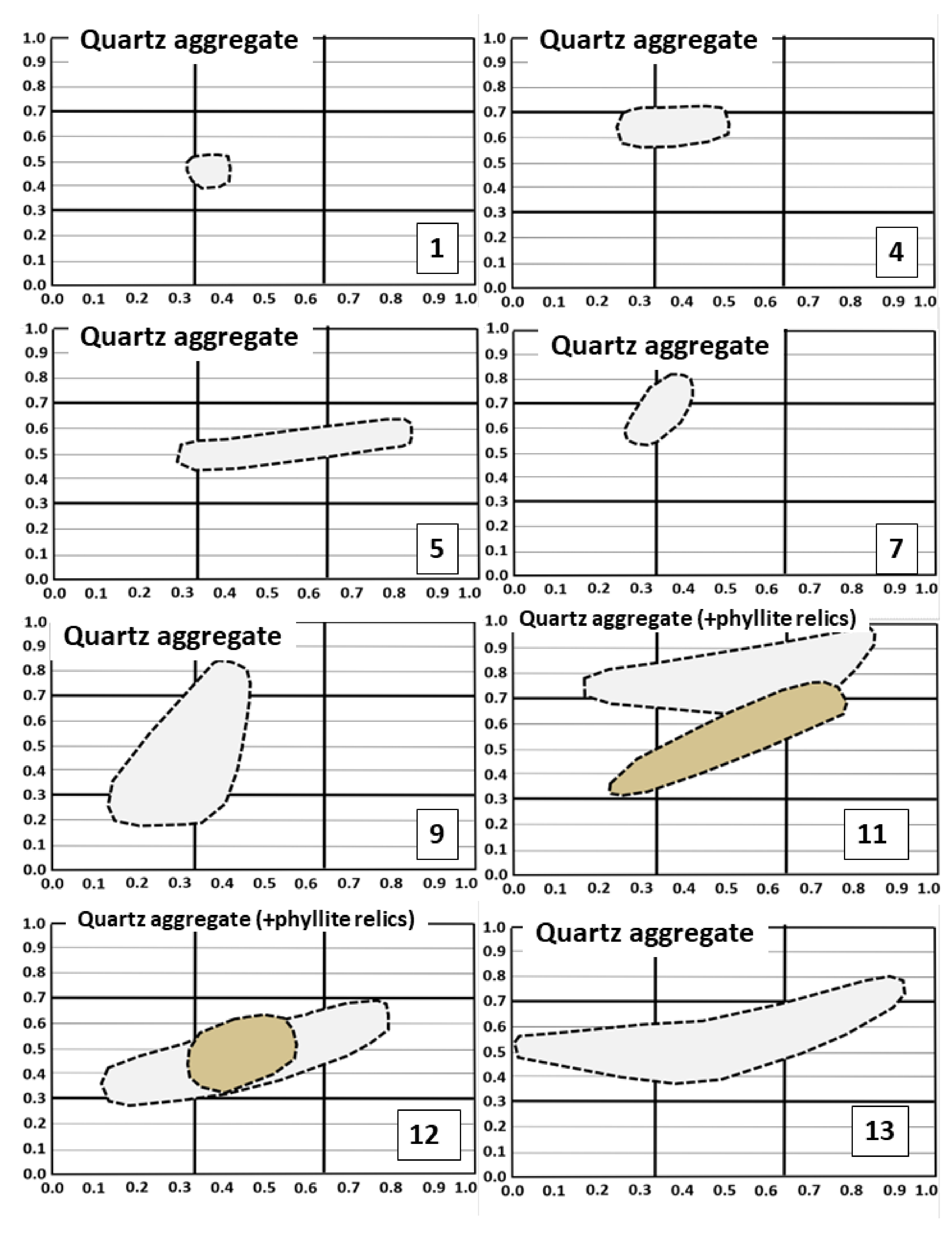
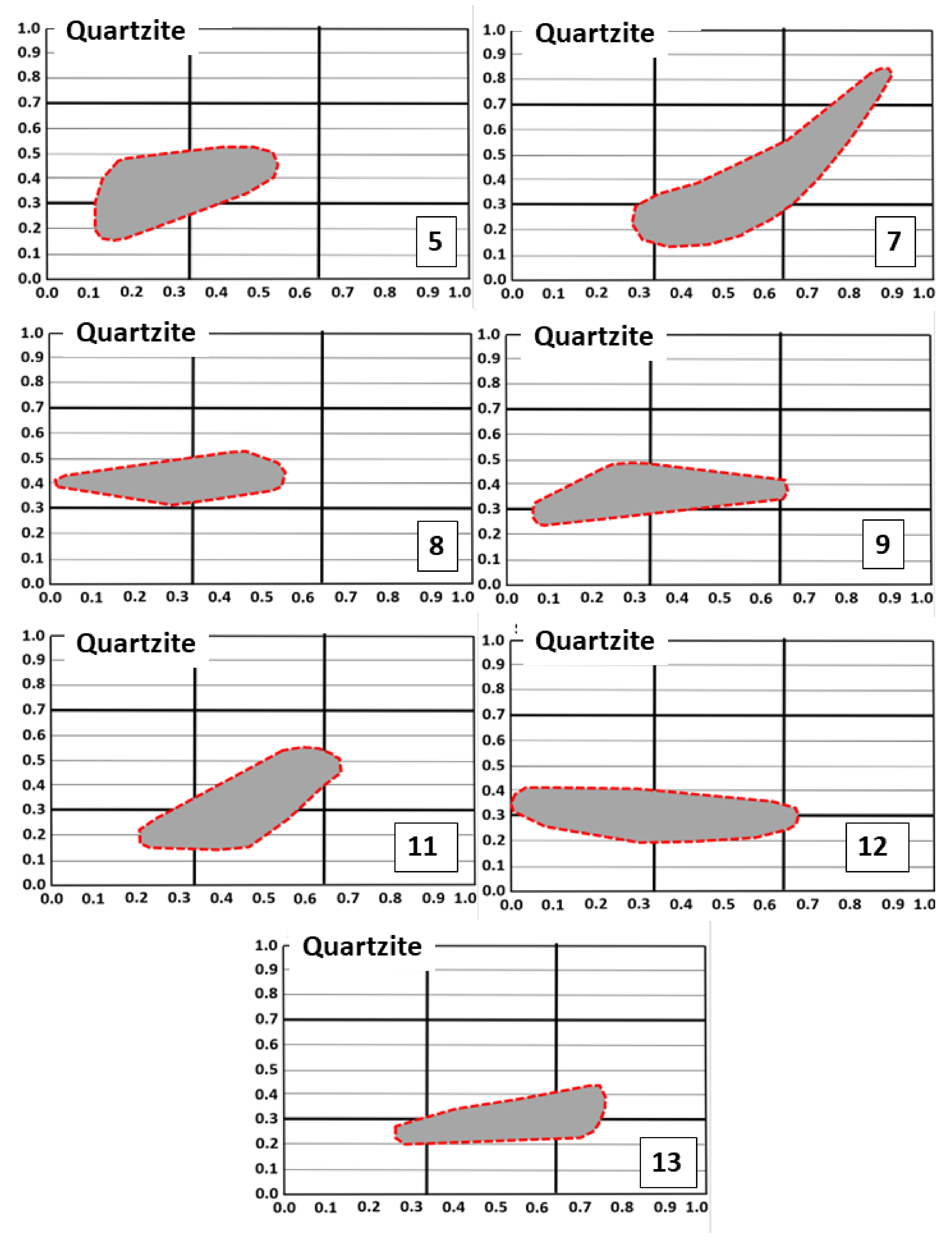
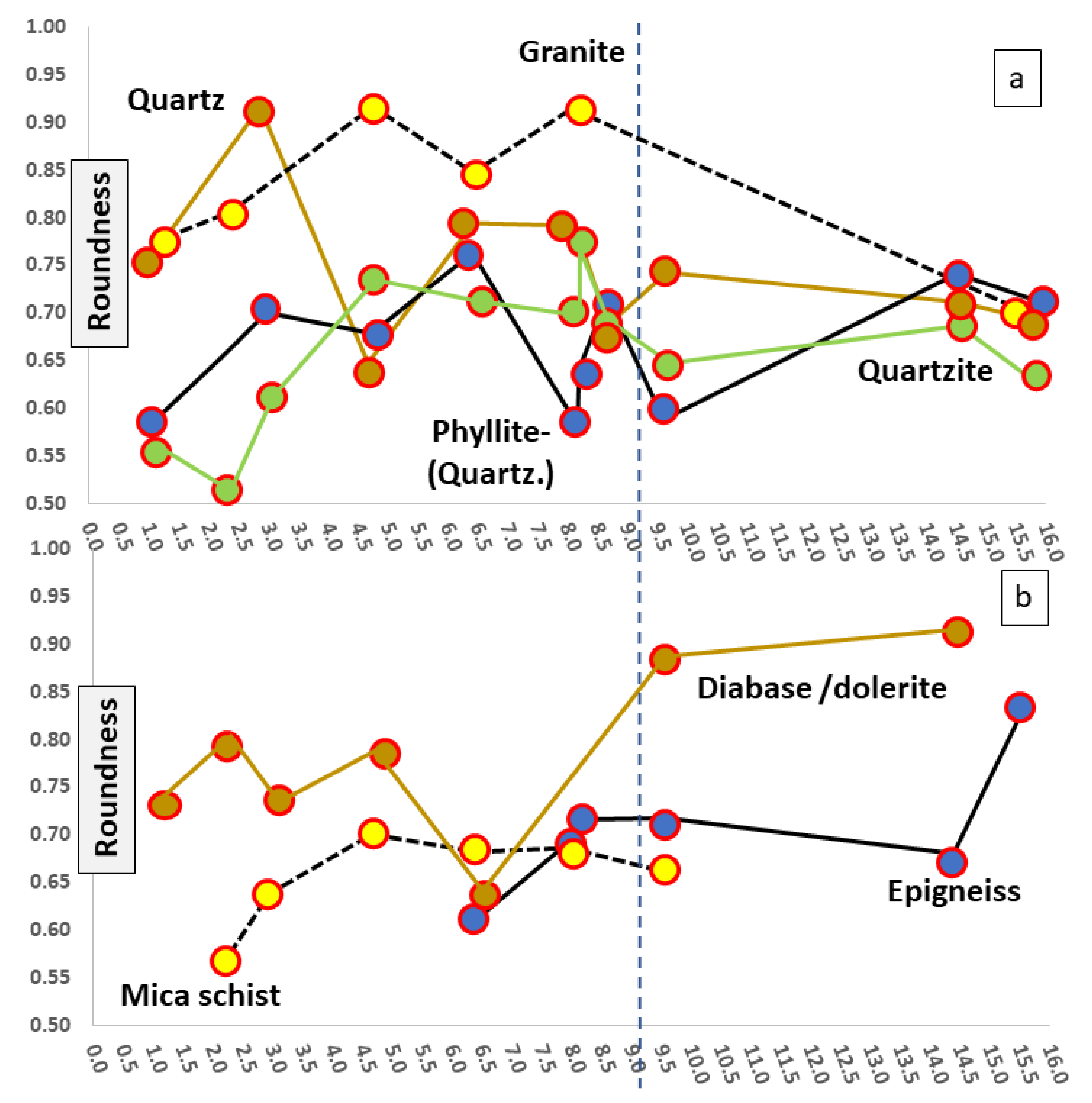
4.3. Grain Morphology of the Gravelly Debris

More than granulometry and situmetry, the grain morphology is linked to the mineralogical/lithological composition of the coarse-grained sediments as demonstrated by the three methods applied in the current study: (1) visual examination of the roundness index after Powers [23,85], (2) triaxial measuring the three dimensions of the particles after Illenberger [24], and (3) digital image analysis determining the circularity, aspect ratio, roundness, and solidity (Figure 6, Figure 7, Figure 8, Figure 9, Figure 10, Figure 11 and Figure 12). A description of classical methods No. 1 and No. 2 is provided by Boggs [86]. It has to be noted that the sequence of methods does not mirror an evolution of sedimentological parameters from the analogue towards the digital sedimentological world, but every method still has its advantages today which can best be harnessed by a tripartite approach taken in the field and in the laboratory. The most recent successful use of morphological studies of fluvial gravel clasts has been achieved in Holocene sediment of the Sava River, Croatia, by Barudžija et al. [87] who made use of the x-y plots elaborated by Zingg [88]. An overview of the methods available to determine the shape of grains in sedimentology has been given by Blott and Pye [89].

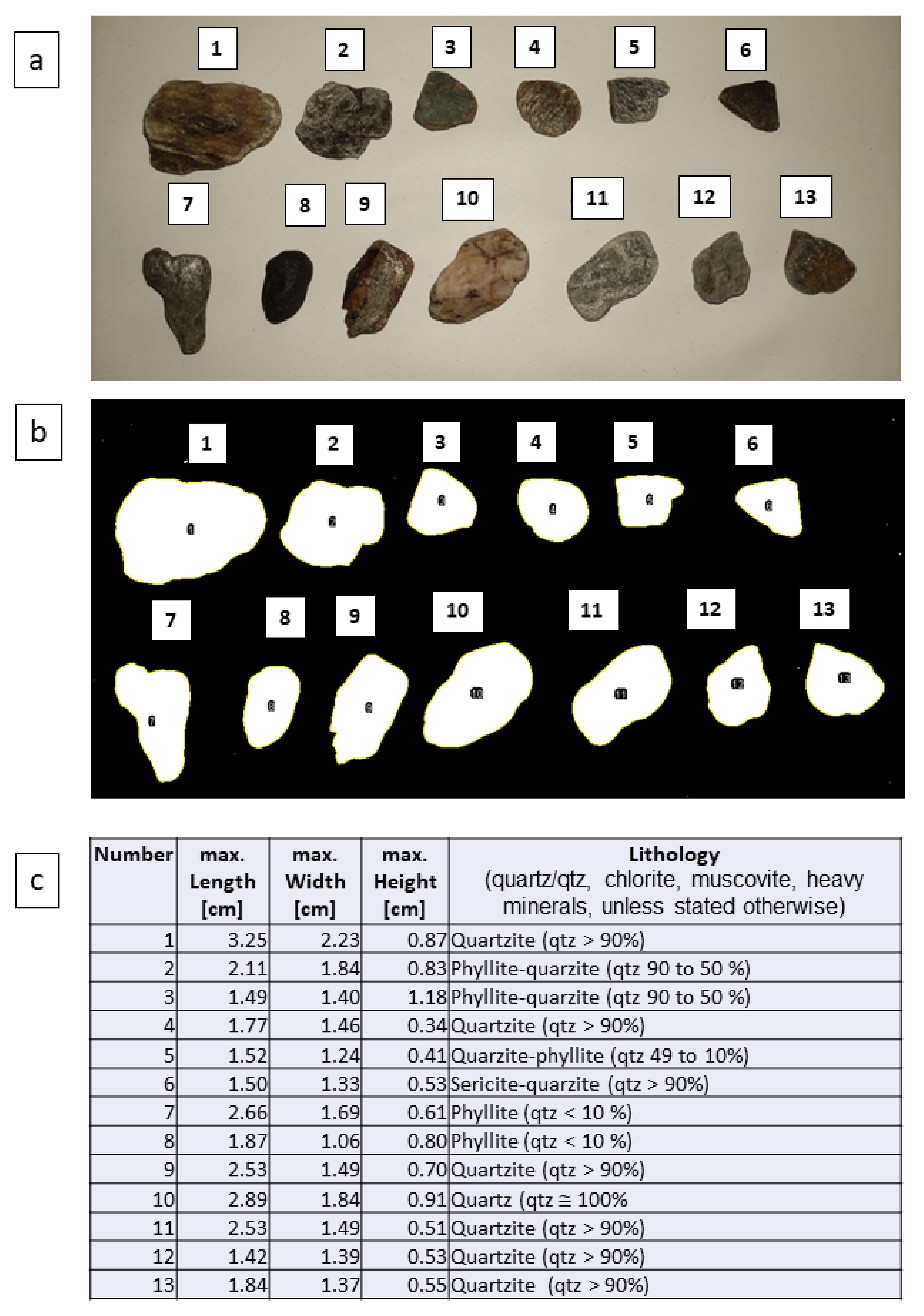
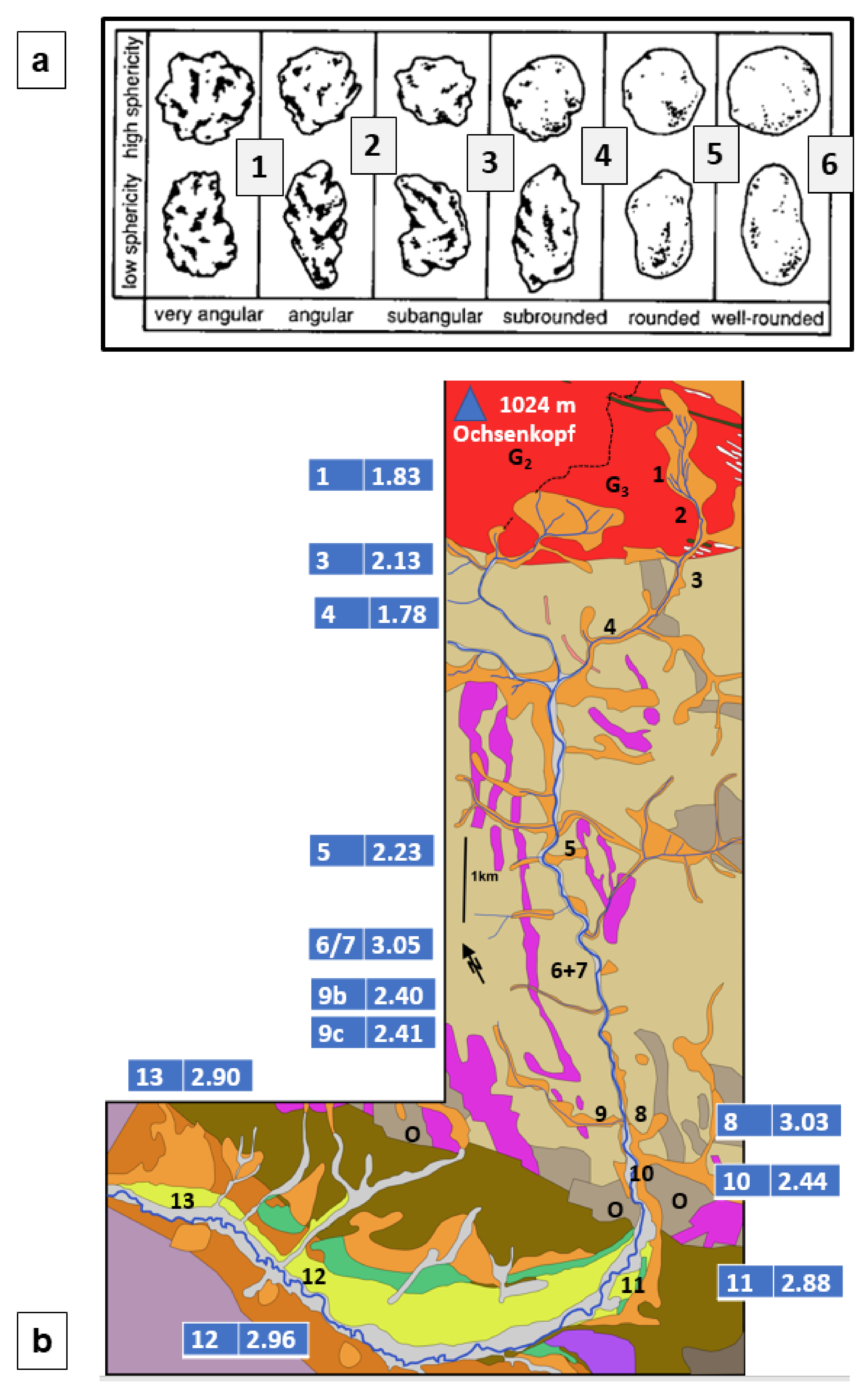
4.3.1. 2-D Visual Examination and Comparison Charts

The roundness of the gravel-sized detritus is determined on the basis of comparative charts showing six reference grain classes, each of them subdivided into gravel-sized fragments of low and high sphericity gravel [23,85]. To allow for a numerical comparison, each class is assigned a number, giving the very angular-shape class the number 1 and the well-rounded one at the opposite end of the scale the number 6 (Figure 10a). The mean of roundness can be calculated and plotted for each sampling site as a function of the distance to source and fluvial facies (Figure 10b). A general trend of the roundness to increase downstream from angular (>1.5) to subangular (>2.5) can be inferred but exceptions from this rule have also been considered midway between two intermediate sediment traps where the roundness reaches the subrounded level.

4.3.2. 3-D Measurement of Shape and the Morphology Indices

The 3-D measurement of the small (S), intermediate (I) and large (L) size/axis of the gravel debris by means of a yardstick or caliper is the basis for the calculation of the disc-rod index ((L − I)/(L − S)) and the shape index (S/(I × L)^1/2 (Figure 6). The most widespread lithologies in the western Fichtelgebirge Mts., the granitic intrusive rocks and the surrounding meta-pelitic rocks show rather regular trends and data arrays in the x-y plots of Figure 7. Granites have high shape indices except the granitic gravel of site 13. Quartz aggregates with and without relic phyllites are shown in Figure 8. By comparison with the phyllites, the shape patterns of quartz aggregates are less variegated than those of the metapelites. Not surprisingly, these monomineralic aggregates form the “positive boomerang pattern” (Figure 8—site 13), small isometric clusters (Figure 8—site 1) or inclined ellipses (Figure 8—site 5), all of which with high shape indices relative to the meta-pelitic rocks. Quartzites only play a part relatively late within the longitudinal fluvial profile owing to the poor exposure of meta-psammopelitic rocks in the upper reaches of the Steinach River (Figure 9). Apart from the morphological patterns referred to previously, the quartzite data cluster subparallel to the x-axis at rather low shape indices (Figure 9—site 12) and also form the “negatively skewed boomerang pattern” (Figure 9—sites 9, 11).

4.3.3. Digital Image Analysis

The digital image analysis offers a great variety of parameters to describe the shape of gravel and also paves the way into the granulometric section of the GMS approach. In Figure 11, a reference example has been selected for a direct comparison between the 3-D and 2-D methods, tackling the morphological issue.

Morphological studies of grains are often conducted using different techniques in image analysis [90,91]. Visual inspections using morphology charts proposed by Illenberger [24] and measuring the tripartite set of dimensions, the smallest, intermediate and longest axes are two options indicating a sequence towards gathering numerical data. The digital image analysis measures five parameters: (1) area, (2) circularity, (3) roundness, (4) aspect ratio, and (5) solidity (

Table 2. Lithology of gravelly debris of the Steinach drainage system and the mean values of different sedimentological parameters measured and calculated from digital image analyses of gravel. For definition and algorithm of area, circularity, aspect ratio, roundness and solidity please see text (Section 4.3.3, Digital image analysis).

Lithology of Sediment Grain	Area	Circularity	Aspect Ratio	Roundness	Solidity
Granite (in places pegmatitic)	12,600	0.774	1.241	0.819	0.958
Metavolcanic rocks (basic)	5165	0.748	1.314	0.792	0.948
Diabase plus “Proterobase” (diabase/dolerite in dikes)	11,218	0.783	1.322	0.781	0.961
Quartz aggregates (in places with relic phyllite fragments), quartz monomineralic, red-pinkish (e.g., carnelian, jasper), milky vein quartz	8557	0.772	1.401	0.738	0.954
Mud clasts	3164	0.721	1.388	0.736	0.914
Graywacke	11,166	0.748	1.378	0.734	0.947
Epizonal gneiss (“Epigneiss”)	8911	0.805	1.43	0.713	0.971
Mica schist	9201	0.798	1.529	0.674	0.972
Phyllite, phyllite with remnants of quartzite, phyllite sheared (phyllonite)	10,316	0.773	1.557	0.673	0.964
Fault breccia	2371	0.773	1.508	0.663	0.947
Quartzite, quartzite-phyllite, quartzite intergrown with remnants of phyllitic aggregates, sericite quartzite, quartzite with trace fossils “Phycodes Quarzite”, quartzite + ferricretes	9404	0.748	1.622	0.658	0.953
Conglomerate	12,363	0.746	1.564	0.639	0.951
Ferricretes	7225	0.722	1.801	0.621	0.946
Sandstone	5769	0.753	1.67	0.599	0.969
Limestone calcitic to dolomitic	4814	0.699	2.069	0.489	0.946
Calcite aggregates	14,875	0.648	2.243	0.446	0.939

). Tests throughout this study revealed the circularity (sphericity) and roundness (roundness-angularity) out of the group of the aforementioned parameters, which are used for a great variety of scopes outside geosciences, such as internal surgery [92].

Aspect ratio is defined as the ratio of major axis to minor axis. It comes close to the method described in the previous section which considers all three axes. This parameter is therefore held to be redundant and not further debated in-depth, excluding the small gravelly lithoclasts of the pebble-size clast community where manual handling often is too time-consuming and rather complicated.

Solidity is defined as the area divided by a convex area. It has proved to be the least meaningful among the cited and tested parameters.

Circularity is defined as 4 π · A/P2, where A is the area, and P is the perimeter of the grain. Values close to 1.0 are close to a perfect circle. As the value approaches 0.0, it indicates a grain with an increasingly elongated shape.

Roundness is defined as 4 · A/(π · x2), where A denotes the area and x the major axis. Roundness and circularity are strongly positive correlated (R² = 0.4629) and consequently only the roundness, which is more sensitive to environmental changes, is applied in the current study (Figure 11a,b). In Table 2 these parameters are listed side-by-side each for the lithologies determined in the drainage system, so as to allow a direct comparison. There are two different groups of gravel lithologies, synonymous with the main lithoclasts types, that show different trends in their roundness when plotted versus the talweg downstream at the basement-foreland boundary (Figure 12a,b). Diabase/dolerite and epigneiss reveal a positive trend downstream with a remarkable increase in roundness. This also holds true, albeit not very strikingly, for the mica schists. There is a conspicuous maximum in the graphs of the metapelites, while showing an overall positive trend towards an increase in roundness. Granite and quartz aggregates reflect a similar hump; however, with a tendency of decreasing roundness values downstream (Figure 12a). The hump coincides with the appearance of the intermediate sediment traps and the zone where the steep gradient flattens (Figure 5 and Figure 12).

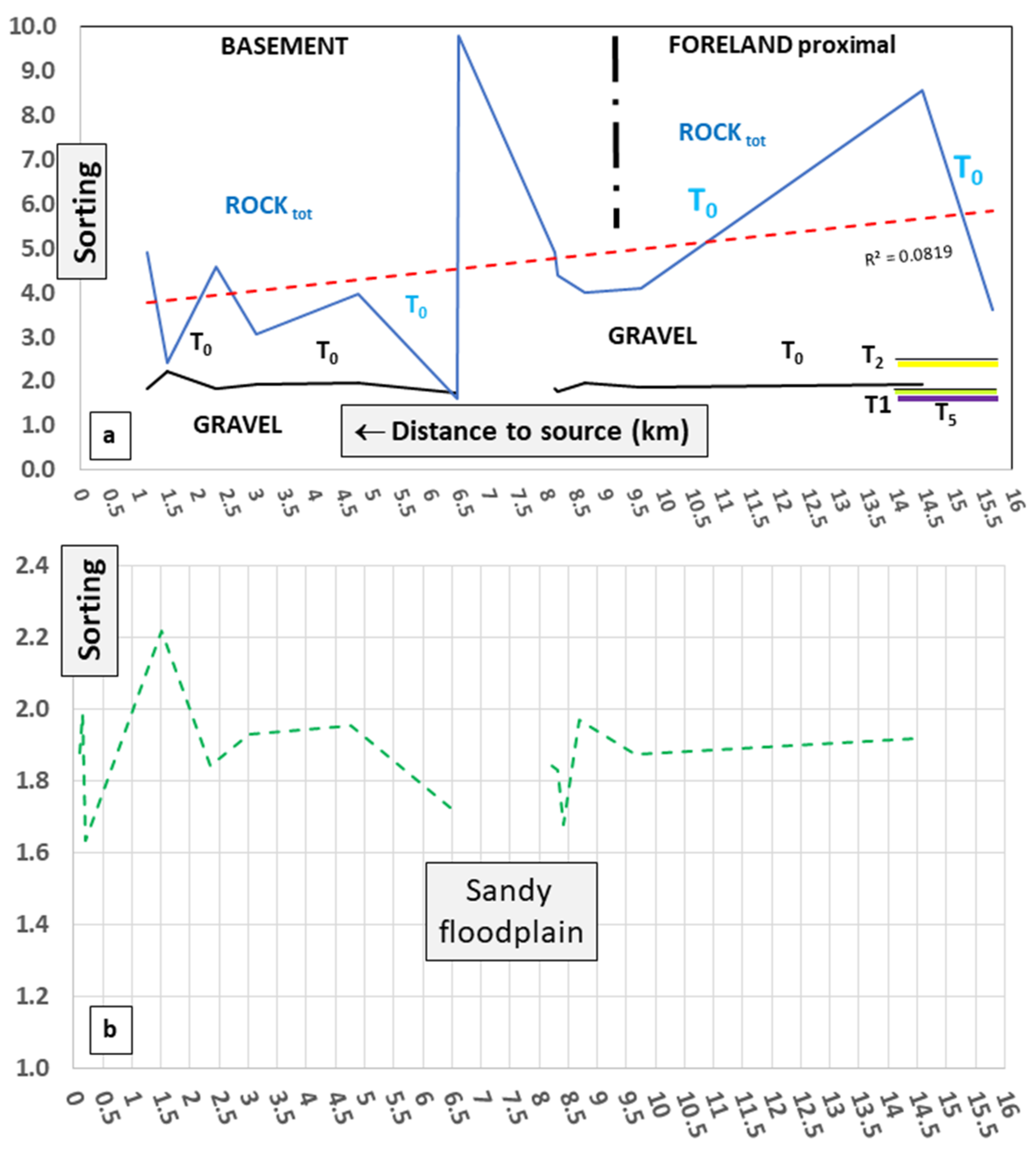
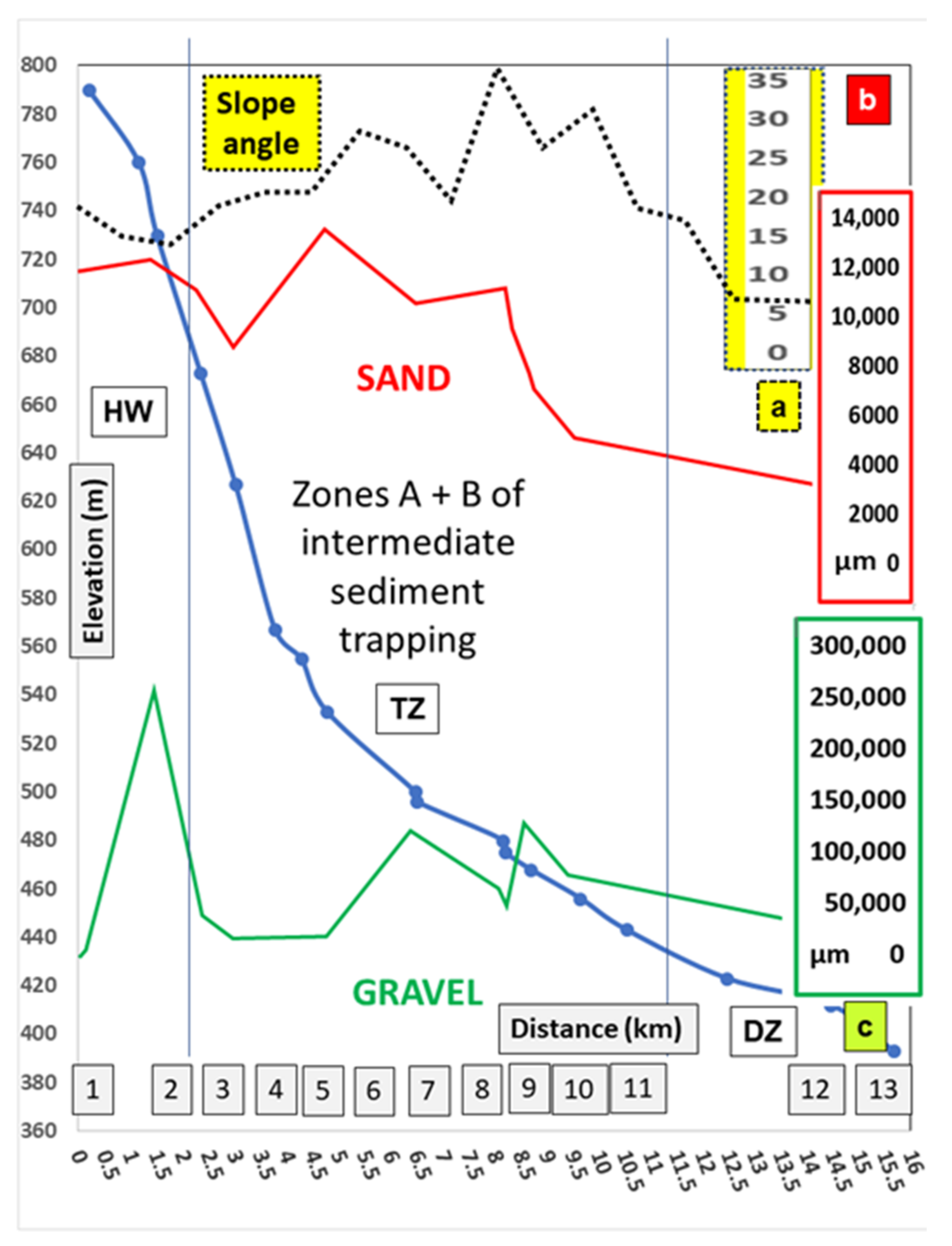
4.4. Granulometry of the Gravelly Debris

The analysis of grain size pertains to the sedimentological methods that can look back on a very long history [11,12,13,14,15,16,17,18,19]. Although being directly related to the various sedimentary environments of deposition, the existing transport agents, such as wind, ice and water, the length of transport distance and time of attrition, the overall increase in computing efforts and the steady refinement of the complexity of equations through the last decades has neither lead to a significant clarification of the influence of the various factors on the grain size distribution nor substantially contributed to the marker effect of granulometry as it is used as a stand-alone approach [93]. In the current study the method is not restricted to the gravel size range and combined with an analysis of the landscape forming the platform of the land-forming processes. Some common parameters of coarse-grained sediments, such as sorting, are used together with the equivalent parameter of the smaller sand fraction. An extension of parameters, such as skewness and kurtosis, did not refine the environment analysis, either. Tests revealed that the application of histograms and frequency distribution curves in plain view or maps similar to the use during morphometry are less meaningful than for morphometric and situmetric studies. As demonstrated by the succeeding examples, plotting the granulometric data as a function of the paleo gradient and the slope angle obtained from the terrain analysis proved to be of assistance when using this sedimentological method aimed at environment analysis (Figure 13 and Figure 14).

The sorting of gravel is rather uniform compared to that of the sand fraction with only a few deviations from the horizontal graph, the most significant of which is between 730 m and 770 m above mean sea level (a.m.s.l) where the boulder strewn gently tilted plain turns into grusy sediments blanketing the top slope (Figure 5). There is another jump towards a refinement of sorting in the middle stream sections between 440 m and 550 m a.m.s.l., where a floodplain evolved instead of longitudinal bars known from up and downstream (Figure 5 and Figure 13). In both sections the mean of the grain size goes through a relative minimum (Figure 5 and Figure 14). A closer look at the whole rock sorting (sand plus gravel) provides a contrasting picture, with a sudden increase in the sorting values where the pure gravelly sediments are well sorted (Figure 5 and Figure 13). The clue to this phenomenon may be deduced from the graph illustrating the change of the slope angle along with the talweg. At sampling site 8 the slope angle attains its maximum of 35°; in other words, a wide valley narrows down to a V-shaped valley, creating some kind of a pool confined up and downstream by steps and cataracts (Figure 5 and Figure 14).

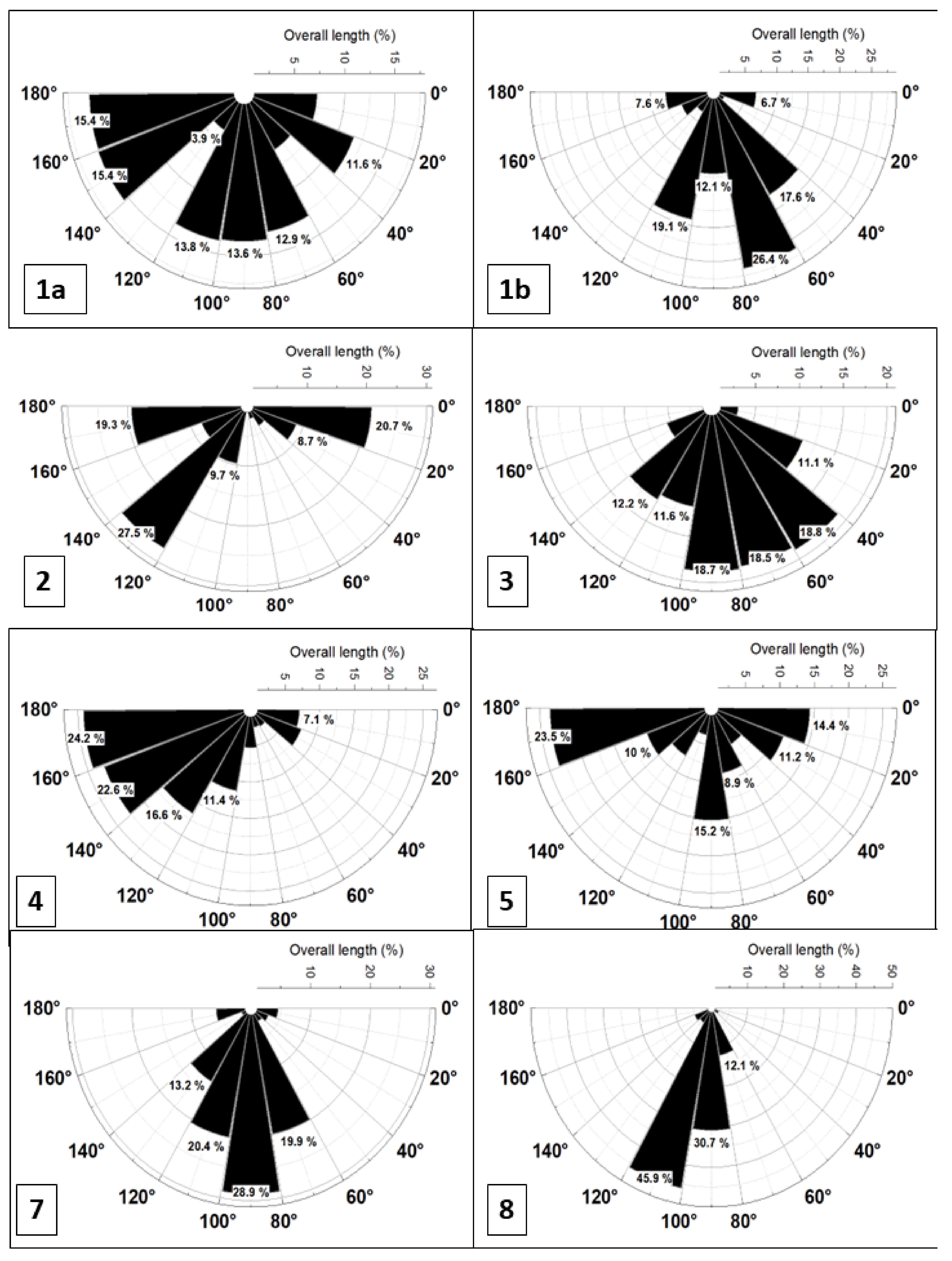
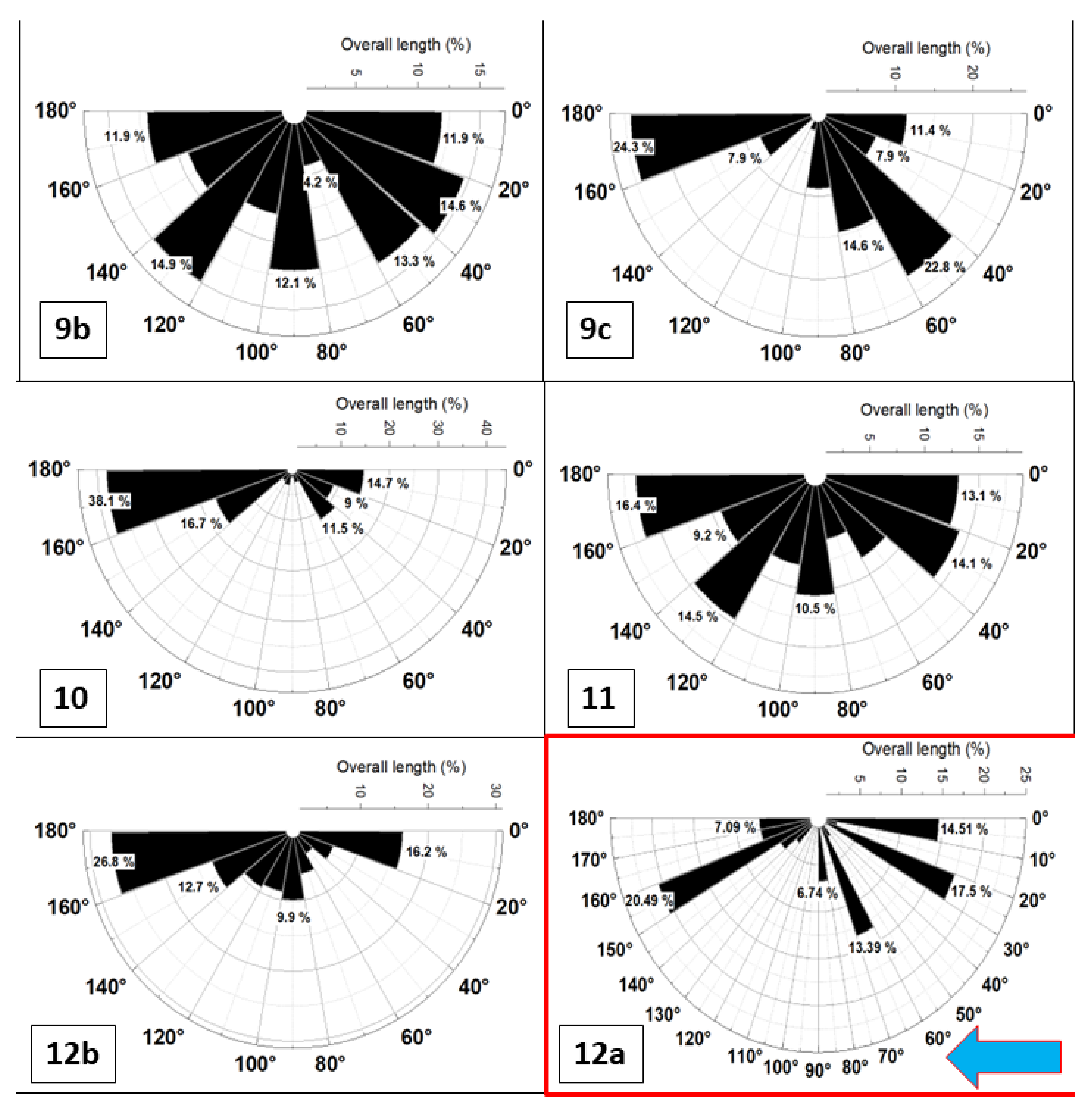
4.5. Situmetry of the Gravelly Debris

The clast orientation is another string to the bow of the GMS method and in the majority of cases used as a tool by glaciologists and volcanologists [95,96,97,98,99]. Little is, however, conducted outside these environments of formation mentioned above [45,46,47,100,101]. The horizontal semicircle rose diagrams are arranged at each site perpendicular to the channel axis of the drainage system, excluding site 12a where the baseline 0–180° of the vertical diagram is arranged parallel to the flow direction of the river (Figure 15 and Figure 16).

Several tests with semicircle and mirror rose diagrams proved the semicircle rose diagrams with sectors measuring 20° to be the most suitable ones for horizontal gravel patterns to unravel the main processes of deposition. In vertical sections parallel to the paleocurrent, semicircle rose diagrams with sectors at an angle of 10° provide reliable results (Figure 15). The latter approach is the only efficient way to gain an idea of the hydrodynamic system in the stacked patterns of terraces in the proximal and distal foreland incised by the upper reaches of the Main River (Figure 2 and Figure 15) [47]. The various diagrams of the horizontal situmetric measurements are given in Figure 15.

The horizontal diagrams rarely show up as a single-sector diagram with one 20°-sector totaling 100%, The common appearance observed in the semicircle rose diagram is that of a “fan-shaped” pattern, achieving the maximum possible of the “fan-sector-percentage-value” of 180°. Sectors of less than 5° are not considered in the calculations because they have proven to be what might be called “noise”. In practice, a first order fan with or without a second order fan of lesser intensity are encountered in the field. Going any further and conducting a more subtle interpretation of the horizontal 20°-semicircle diagram would have meant exaggerating their meaningfulness. Considering the horizontal diagrams and categorized with regard to the arrangement of maxima (1) discrete unimodal maximum fan types and (2) polymodal maxima fan types can be found (Figure 15—sites 8,9b). With regard to the fan shape, a second order subdivision into symmetric (Figure 7 and Figure 15) and asymmetric patterns (Figure 8 and Figure 15) can be accomplished. Another numerical parameter is the “fan intensity” which is given in percentage values covering the overall fan, excluding those sectors of less than 5 %. Not surprisingly, the majority of cases under study, however, are composite situmetric types, reflecting a combination of basic types, which are going to be discussed later in the study for their environment of deposition, see Section 5.

To disentangle the various semicircle rose diagrams, some numerical approaches have been selected and defined to decipher these sedimentological diagrams so as to be useful for an environment analysis (Figure 17, Figure 18 and Figure 19). They combine the orientation and their quantity of the clasts within the first and second order fans.

To show the geographic arrangement of the fans in the map, the orientation indicated by the clast imbrication of the first and second order maxima are plotted relative to the strike of the talweg in an x-y plot which is shown vis-à-vis the gradient and the sedimentological parameters, such as the sinuosity, the sediment traps of fluvial and mass wasting deposits (Figure 17). The angular deviation of the first and second order maxima from the river course varies between 90° and 0°, with regular antithetic trends that show a good match to the topographic and sedimentological data (Figure 18).

The frequency distribution of the clasts and shape of the fans is called the “fan sharpness” which, by definition, is the “fan intensity” given in percentage (see above) divided by the “fan sector”, measured its full angle. It varies in the setting under study between 0.527 observed in the second order fans and 2.664 calculated for the first order fans (Figure 19a,b).

On account of the poor outcrop situation, which are normally found in sand pits and trenches and created on purpose, the vertical situmetry is somewhat underrepresented and reference sites can only be recorded from outside the study area, from the distal foreland zone and discussed together with the dataset of site 12a of Figure 16 [41].

5. Discussion

5.1. The Natural Processing Plant—Compartmentalization and Grain Size Distribution

The master drainage system is subdivided into three compartments, named headwaters (erosion >> deposition), transport zone (erosion > deposition), and deposition zone (deposition ≥ erosion), complemented by several rivulets and creeks tributary to the master stream. The boundaries of the three hydrographic zones are marked by a change in the cross-sectional morphology of the valley while being numerically backed by a slope angle analysis (Figure 5 and Figure 14). The downstream variation is as follows: Headwaters-transport zone (wide-shallow valley → V-shaped valley at a slope angle of 17°), transport zone–deposition zone (V-shaped valley → asymmetric valley with depositional terraces evolving on the low scarp at a slope angle of 6 to 8°) (Figure 14). The headwaters are characterized by an alluvial to non-alluvial dendritic channel system which evolved on a subhorizontal planar erosional landform termed peneplains [102,103]. It was subsequently undergoing a periglacial reshaping leading to the formation of local nivation cirques [42,104].

The change from the CA (catchment area) into the TA (transport area) and from the TA into the DA (deposition area) is marked by abrupt grain size increases caused by changes in the gradient and the presence of knickpoints.

The gravel clasts show a conspicuous grain size “jump” downstream of knickpoints within the talweg at the boundary from the headwaters to the transport zone, where the maximum in grain size and accumulation of grus was achieved (Figure 5 and Figure 14) [105]. It is controlled by the litho-variance (granite → metapelites abundant in quartzites) and tecto-variance manifested by a series of hematite-bearing quartz veins controlled by some normal faults (Figure 3). A second maximum occurs in the transport zone where the intermediate traps A and B are located (Figure 5 and Figure 14). It is the section of the talweg where the sandy matrix was separated from the coarser lithoclasts prior to the gravel enrichment and the narrowing of the valley down to a gorge, which is indicated by the maximum of the slope angle attained at a slope angle of 35° (Figure 5 and Figure 14). This natural dressing plant shows three different intermediate sediments traps, changing from a “whirl-pool trap” A, through a “flood plain trap” B, rife with sand, into eventually a “terrace trap” C. The latter extends across the Weidenberg Bowl and forms part of the deposition zone. In the sediment trap B, the V-shaped valleys also host the true placer ore deposits attesting not only to y differentiation by grain size, but also specific gravity as demonstrated by the accumulation of the heavy minerals, barite and siderite [74,106,107]. The sediment trap B is also the one where the difference between the sorting of sand and of gravel runs through a maximum (Figure 13). A second maximum of that kind can be observed in the depositional zone of the sediment trap C where the stacked pattern of terraces begins. Its differentiation is less strong because of the widening of the valley which provokes a dilution rather than an accumulation.

5.2. Provenance Marker and Grain Morphology Distribution

The morphology of heavy and light minerals has frequently been used during provenance studies in the majority of cases within context with a meticulous mineralogical study and backed by micro-chemical analyses’ heavy minerals [108,109,110,111,112]. Lithoclasts in the channels are closely linked to the wall rock lithologies exposed along the valley slope and as bedrock incised by the river forming in the straight to low sinuosity channels; typical step-and-pool couples with a spacing from the centimeter to the meter scale. These washboard structures or riffles acting as a “natural sluice box” influence the size and the shape of fragments. In contrast with the large number devoted to mineral grains, the number of similar morphological analyses on gravel-sized lithoclasts is rather small and warrants a more detailed discussion herein [87,113,114,115]. Apart from the outcrop scenario, the morphology of lithoclasts is affected by the primary lithogenic and secondary tectonic processes. Both processes are overprinted by physical and chemical supergene processes, the influence of which is on the rise, along with the distance of transport and the time of exposure to chemical weathering. The morphology of the main lithoclasts granites, phyllitic meta-pelites, silica aggregates, and quartzitic meta-psammopelites described in the Figure 3 may also contribute to shedding some light on the evolution of the landscape during the Quaternary and Neogene.

The granites, albeit taking an outstanding position in the landscape while forming the highest summits of the Fichtelgebirge´s granite cupolas, have only a moderate preservation potential among the gravelly lithoclasts of the drainage system which is a function of grain size. Large boulders originating from the “Kerngranit” (core granite G3) are of widespread occurrence in the headwaters spanning across the relic peneplains of the Neogene age at a height above 740 m [57,58] (Figure 4a,h and Figure 5). Their rounded shape is directly related to the tors and woolsacks exposed nearby which, when collapsed under a colder climate, turned into boulder-strewn high-altitude plateaus and blockfields [116,117,118,119]. It is the portion of clasts which shifts the data array into zones A, B and C (Figure 3e). The characteristic towers of woolsacks on the Fichtelgebirge summits displaying subhorizontal onion-shell fractures, sheet joints and subvertical mural joints originating from the cooling history of the granitic magma, and measuring by the meter scale had an effect on the size and morphology of the granitic rock slaps as the granitic rocks disintegrated during the glacial period [59]. The discs and blades, however, have been derived from a different source area (Figure 3—No. 1, 3). It is the G3 areas which were intersected by WNW—striking normal faults which did not only create the vents for dolerite dikes and quartz veins but also converted a significant proportion of their granitic wall rocks into decimeter- to centimeter-sized granitic rock slices which in parts show a greenish tint due to hydrothermal chloritization (Figure 4b,c).

These tectonic and hydrothermal processes coupled with the emplacement of the quartz veins intersecting the granites on a decimeter-spacing and abundant in lustrous hematite provide a lithological prerequisite to form the blankets of grusy granite clasts found in and around the alluvial dendritic headwater channels (Figure 4h) [74,75]. It is the transition from the headwaters into the zone of transport where grus acts as the lubricant for the sliding boulders (Figure 5). Both phenomena can be traced back to the Neogene when a tropical wet and dry paleoclimate sparked a widespread peneplanation; that was the key element for the boulder- and grus-shaped granitic lithoclasts [120].

After a long distance, almost barren of granitic lithoclasts, another granite lithoclast of G2 appears at site 13 in the terraces and the Holocene floodplain of the Steinach River, featuring a shape completely different from that of granite G3 (Figure 3 and Figure 7). It is the result of by-passing processes which began 6 to 4 Ma years ago during the Neogene, when a braided stream paleodrainage system evolved NW of the Fichtelgebirge Anticline and which tapped into the G2 granite [24,53]. This ancient paleodrainage system featuring all hallmarks of a straight to low-sinuosity drainage system widened downstream to a vast braid plain debouching its sediment load in the immediate foreland of the basement. As far as the fluvial type of braided stream is concerned it can be denominated according to [121] as a Scott-type braided stream on account of its poorly sorted and massive to vaguely bedded gravel accumulations. The granite G2 gravel of site 13 was not transported all along the course of the modern Steinach River, but pre-concentrated on the Neogene braid plain which, when dissected by the Steinach during the Quaternary, picked up these pre-shaped gravel clasts. In both granitic suites, the strong impact of mass wasting is indicated, whereas the short-distance fluvial transport is almost negligible as far as the transport is concerned. Mass wasting, be it a slow-motion talus creep or fast-moving slurries of a debris flow, has a much higher shape-preserving capability than fluvial processes in a straight non-alluvial drainage channel.

The mica schists or chlorite-bearing phyllite metapelites are more heterogeneous than the granites owing to their heterogeneous parent material and were tectonically more strongly impacted by the Variscan Orogeny during the Late Paleozoic than the post-orogenic granites, which were only faulted near their margin [122,123]. Their common “boomerang pattern” (disc-blade–elongated sphere) attests to a more or less positive correlation between the shape- and disc-rod indices. The positive correlation shifting the data array into the compartments C, D, E, F, and H is due to a stronger deformation with the formation of microfolds, phacoids and boudinage (Figure 4d,e).

Only at site 4 platy phyllites show up markedly different in shape from the overall data arrays. In this setting, close to the granite, the low-grade regionally metamorphic phyllites were altered by a contact metamorphic overprinting by the granite G3 and given a hornfels-like outward appearance without any conspicuous mineralogical changes. The morphological data arrays of the metapelites were adjusted to the data array of granites despite their strong compositional difference (Figure 3). This low grade metapelite–hornfels has the highest shape index which is indicative a higher temperature regime conducive to a higher rock strength. Considering the metapelites, an increasing shape index while the disc-rod index is left unaffected points to a higher temperature imparting a more felsic outward appearance to the lithoclasts (Figure 6). Metapelites can be observed all along the talweg far into the distal foreland, with the maximum distance achieved 100 km off the source area in the “Bamberg Bowl”, where metapelites, however, are recognized no longer as metamorphose argillites but among the quartz aggregates where discrete chlorite flakes in vugs and notches clearly attest to the parent material they have been derived from (Figure 4f).

Quartz aggregates are common constituents of the gravel-sized lithoclast assemblages with diagnostic features, each of which are indicative of the parent lithologies (Figure 8). Site 1 and site 4 clusters overlap with their parent lithologies, granites, including their quartz veins, and the phyllite hornfelses, respectively (Figure 3 and Figure 7). For sites 11 and 12, quartz aggregates bearing voids filled with chlorite flakes and quartz phyllites are plotted in the same x-y plot to show that they are genetic kindred entities which move closer to each other on fluvial transport, eventually causing the quartz aggregate to mimic the “boomerang-shape” cluster pattern of their parent metapelites which they have been derived from.

The meta-quartzites are nothing but the end-member types reflecting the arenaceous parent rocks of the meta-psammopelitic suite of country rocks around the granite domes. There are two series as to the position within the transport zone and the morphology. Quartzite sampled at sites 5 and 7 have a rather high shape index and originated from source rock next to the granites, whereas the remaining samples stem from the platy quartzites, mainly of Ordovician age, which crop out along the highland boundary fault (Figure 9). The rigid layered meta-quartzites were left undeformed by the Variscan fold deformation and only affected by moderate faulting at their rims. As a consequence of this, their data clusters run parallel to the disc-rod index as a manifesto of a rather low temperature origin.

The morphological variation of lithoclasts along the talweg illustrated in Figure 10 shows an overall downstream improvement of the roundness towards subangular to subrounded, a similar geological setting to the one recorded by Macurová [124]. The decrease in the sinuosity which provokes the flow speed to increase produces an incremental roundness value. This is the case between sites 6 and 8 as well as downstream of site 11 while entering the Permo-Mesozoic foreland. As for the gradient, it is the knickpoint between the headwaters and the transport zone and the entrance into the zone of intermediate traps that have a shape-controlling effect. It is further evidence that this drainage system does not act as a simple “conveyer belt” transporting steadily and continuously material downstream, but more as a “processing plant” with compartments (traps) acting as “crushers”, “ball mills” and “filter systems” all in one.

Considering the morphological parameters of pebble-sized lithoclasts shows the granitic clasts to attain the highest circularity, roundness and solidity while achieving the lowest aspect ratio, which is in full accordance with the highest shape index (Table 2, Figure 7). At the opposite end of the morphological scales, calcareous lithoclasts are found, whereas meta-psammopelites occupy an intermediate position based upon the rock strength.

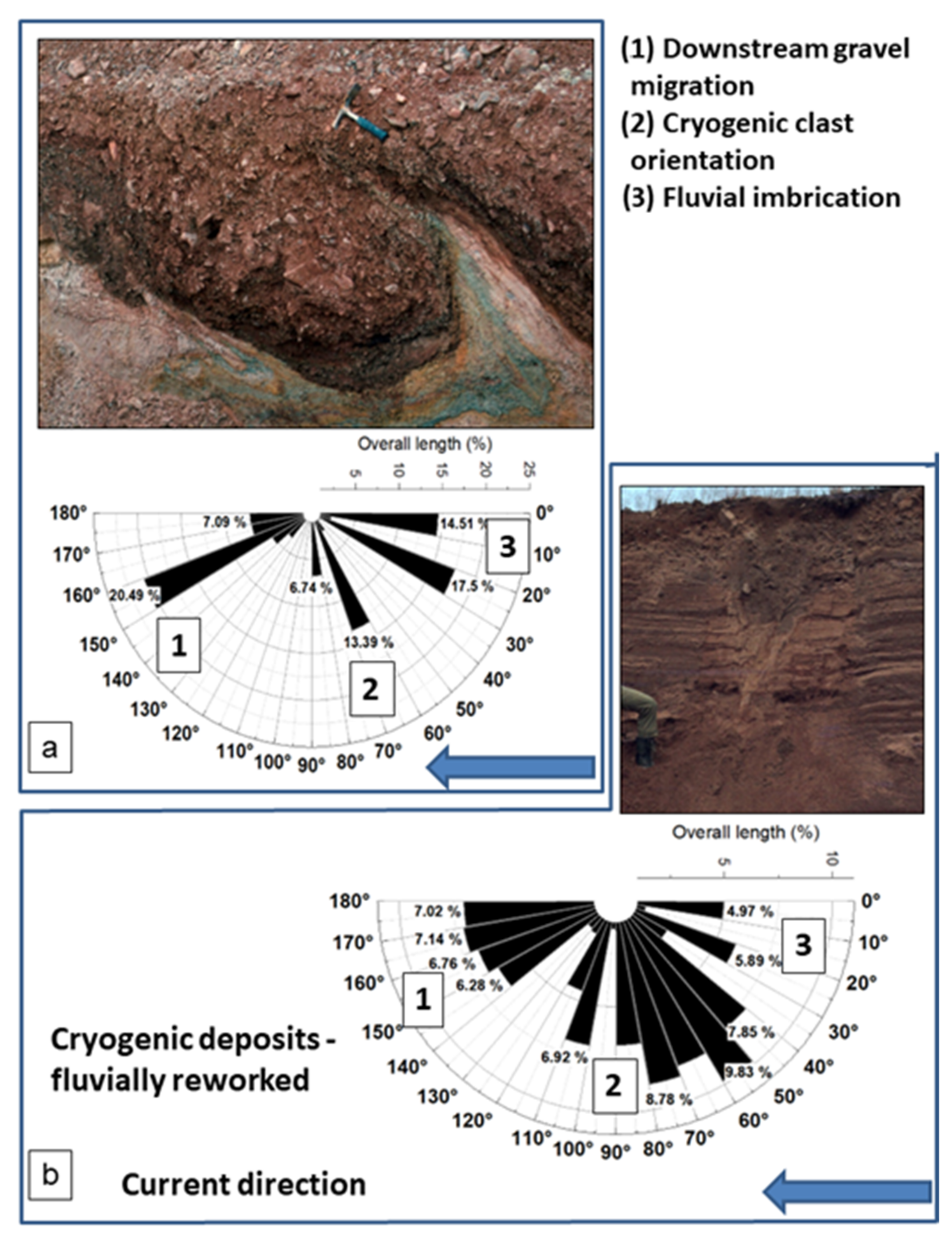
5.3. Hydrodynamic Facies Analysis and the Orientation of Clasts

5.3.1. Clast Orientation in Plain View

Situmetry constitutes the logical synopsis of the GMS laboratory because it well combines the outstanding features of its sister disciplines’ morphometry and granulometry and integrates them into the terrain-analysis by its topographic link. It harnesses the morphological features of lithoclasts characterized by a moderate shape and high to moderately high disc-rod index (Figure 6 and Figure 7) while its image analysis yields a moderately low aspect ratio (Table 2). Measurements of clast orientation can most suitably be applied to lithoclasts in the grain size interval from very coarse pebbles to small cobbles. Larger gravel-sized lithoclasts are too static and difficult to move to gain sufficient measurements to be considered as reliable results. The smaller sand-sized particles, however, can only be handled in this scope by universal-rotating-stage methods following laborious sampling, e.g., using oriented lacquer peels and taking an approach similar to that of structural geologists [125]. The semicircle-rose diagrams are selected and transformed into a couple of distance-angle plots and distance-sharpness plots (Figure 17, Figure 18 and Figure 19). The abrupt change of the river course between sites 10 and 11, which marks its crossing from the basement into the Permo-Mesozoic foreland, also finds a direct response in the clast orientation of the first and second order fans of the coarse-grained straight basement and moderately strong meandering foreland rivers (Figure 17). The horizontal fan pattern cannot be interpreted with the sedimentological parameters of the straight and meandering river sections. The straight channel type, which is a rather instable channel type, has been the subject of indoor laboratory trials and experiments [54,55]. The coarse-grained meandering stream drainage system has rarely reached the spotlight of fluvial sedimentologists and geomorphologists because the characteristic features are not so well expressed as in its fine-grained equivalent [9,126,127,128]. The distance-angle plots with their first and second order fans are a mirror image of the clasts responding to slow-and fast motion mass wasting in straight to low-sinuosity and moderately meandering drainage systems [41,42]. In the foreland the fans are representative of two different processes, fluvial downstream migration and fluvial accretion, which take place perpendicular to the flow direction at different angles. On the slip bank´s highest convex curvature both directions intersect each other at a right angle. Such high-angle cross-bedding by accretion formed by downstream migration of the leading edge of the chute bars moves towards highest concave curvature of the cut bank. This process occurs only in the foreland, where the fluvial processes are at full swing. The straight river sections are dominated by longitudinal and, to a lesser extent, transverse bars. The differential angle between talweg and fans does not widen downstream but fluctuates at an angle around 90°, providing a measure for the sediment supply and sediment caliber (Figure 18). The stronger the angular deviation the lower the sediment caliber and the sediment supply rate, both of which directly translate into the types of fluvial and mass wasting deposition, which is subdivided into slow motion mass wasting deposits, such as soil creep/solifluction and talus creep, and fast-moving processes, such as debris flows grading into fluvial fan deltas and rotational rock slides and rock fall [129,130].

Another parameter calculated from the situmetric measurements is the “fan sharpness” which, when plotted versus distance to source, coincides with the maximum slope angle of the valley of the straight drainage system. The sharpness of the situmetric fans is the result of a combined effect of mass wasting and fluvial processes. Fast moving mass wasting narrows down the valley width while hard rocks favor the preservation of steep hill slopes. This pinching and swelling of the valley provokes an increase in the flow speed according to the hydrodynamic Bernoulli Effect. Irrespective of the pinching effects on the transit ways from whatever land-forming processes, the sharpness of the situmetry fans positively correlates with the flow rate along the valley section (Figure 14 and Figure 19).

5.3.2. Clast Orientation in Cross or Longitudinal Sections

Semicircle rose diagrams to determine the clast orientation put in a vertical position are applicable only where trenches have been dug or sand open pits occur. This is only viable in one sand pit at 12a. All remaining artificial outcrops are situated out of the study area in Mesozoic foreland sediments (Figure 16). Both reference sites describe the same set of sedimentary structures, with a fluvial downstream maximum, a cryogenic subvertical maximum and fluvial imbrication fan. The fluvial reworking is most powerful in the floodplain at site 12a (Figure 16) and the cryogenic land-forming one is the most prominent process in the site, illustrated in Figure 16b where ice wedges evolved underneath the abandoned floodplain.

5.4. Synopsis and Outlook

The current analysis of gravel-sized lithoclasts proves the results which were obtained over several decades [9]. A stand-alone application of granulometry does not provide unambiguous data useful for any environmental analyses or discrimination of processes. Therefore, the logic tells us to go a step further and take a tripartite approach combining all three disciplines to wipe out their weak points and draw an advantage from their respective strong points (

Table 3. The GMS tool and how it can be used in a basement-foreland transition zone. Objects (green). Methods of the E and E issue (economic geology and environmental geology). Identification of land-forming processes.

Key Processes and Targets	Granulometry	Morphometry	Situmetry
Knickpoints and change of the (paleo)gradient	3	1	1
Sediment sorting	2	1	0.5
Sediment traps (whirlpool, flood plain traps)	1.5	1	2
Tectovariance of the parent rocks	2	2	1
Lithovariance of the parent and source rocks (provenance analysis)	1.5	3	1
Placer discoveries	1	2	2
Identification of vulnerable landforms and areas prone to geohazards	2	2	2
Weathering	2	3	2
Hydrodynamic processes	1	1	3
Diagnosis of mass wasting, fluvial, and cryogenic land-forming processes	0.5	1	3

). A numerical assessment reveals that the methods are almost of the same value (situmetry/17.5 > morphometry/17 > granulometry/16.5). The triplet can achieve good contributions in many aspects but shows significant limitations when it comes to the compositional parameters (mineralogy, geochemistry). Therefore, the entire compositional part represented by and named as sediment petrography has to be handled as a separate entity (Figure 20). The tie line between this sedimentological triplet and sedimentary petrography passes through morphometry [87]. In the current case, it is studied and discussed under separate cover, because it would only dilute the weight put behind the sedimentological triplet, because sediment petrography also encompasses the sand- and clay-sized particles which have no meaning for situmetry handled in the current way; they are relevant for granulometry and they are of high significance for morphometry covering the entire spectrum from crystal morphology of heavy and light minerals [22,24,131,132,133,134,135,136,137,138,139,140].

The third component in the triangle sedimentology (GMS) and sediment petrography is geomorphology which in its numerical type, called terrain analysis, paves the way into geomorphometry, where terrain-related datasets are created but sedimentological and sediment-petrographic datasets are not (yet) considered (Figure 20). The digital terrain model (DTM) of the landscape and morphometrics have often been used in different studies, such as in soil sciences, water resource management and the study of land-forming processes [141,142,143,144,145]. We try and seek a golden harmony between purely descriptive geomorphology with or without age dating and the aforementioned separate entity called geomorphometry. This way has proven to provide the most suitable results, for it has already been applied successfully and used for extractive/economic geology and environmental/urban geology in different countries as shown by some reference types [74,146].

6. Conclusions

The GMS tool is one the three key elements besides sediment petrography and numerical geomorphology of an advanced-level terrain analysis of landform series

The components of the GMS tool, granulometry, morphometry and situmetry, each of which are of almost equal value, have pros and cons. Thus, whenever it is possible, they ought to be used in combination and not as stand-alone procedures.

They can be used for the (1) sedimentological, geomorphological, petrographic and tectonic objects, (2) in applied geosciences for the identification of the accumulation of mineral resources and identification of areas vulnerable to geohazards, and (3) in genetic geosciences for the discrimination of supergene chemical and physical processes.

Granulometry of coarse-grained/gravel-sized sediments can be linked to the smaller sand and clay grain size intervals using the sorting, mean and/or median values for an environment analysis.

Morphometry of coarse-grained/gravel-sized sediments can be linked to the compositional geosciences, mineralogy and geochemistry. The grain shape is intimately connected with the lithology and can be assessed in a comparative way, measuring the axis of the lithoclast or by digital image analysis. Each of these analyses has their individual strong points and are consistent and complementary with each other. They are a favorable tool to supplement the provenance of lithoclasts.

Situmetry is the key element of hydrodynamic research directly building upon its sister methods. They are useful for the identification and quantification of physical land-forming processes using the fan sharpness and the orientation of clast relative to the direction of the talweg. Horizontal rose diagrams are useful for the upper reaches of drainage systems to be of alluvial or non-alluvial types, with vertical ones for alluvial channels in the distal and proximal foreland.

References

1. Wilson, J.L. Carbonate Facies in Geologic Time; Springer: New York, NY, USA, 1975; p. 471. [Google Scholar]
2. Reading, H.G. Sedimentary Environments and Facies; Elsevier: Amsterdam, The Netherlands, 1978; p. 557. [Google Scholar]
3. Tucker, M.E.; Wright, V.P. Carbonate Sedimentology; Blackwell: Oxford, UK, 1990; 482p. [Google Scholar]
4. Galloway, W.E.; Hobday, D.K. Terrigenous Clastic Depositional Systems—Applications to Fossil Fuel and Groundwater Resources Rocks; Springer: Berlin/Heidelberg, Germany, 1996; p. 489. [Google Scholar]
5. Scholle, P.A.; Ulmer-Scholle, D.S. A Color Guide to the Petrography of Carbonate Rocks. AAPG Mem. 2003, 77, 474. [Google Scholar]
6. Jensen, S. Paleontology: Reading Behavior from the Rocks. Science 2008, 322, 1051–1052. [Google Scholar] [CrossRef]
7. Flügel, E. Microfacies of Carbonate Rocks-Analysis, Interpretation and Application, 2nd ed.; Springer: Berlin/Heidelberg, Germany, 2009; p. 984. [Google Scholar]
8. MacEachern, J.; Pemberon, S.G.; Gingras, M.K.; Bann, K.L. Ichnology and Facies Models. In Facies Models 4; James, N., Dalrymple, R.W., Eds.; SEPM: Broken Arrow, OK, USA, 2010; pp. 19–58. [Google Scholar]
9. Reineck, H.E.; Singh, I.B. Depositional Sedimentary Environments: With Reference to Terrigenous Clastics; Springer Science Business Media: New York, NY, USA, 2012; p. 551. [Google Scholar]
10. Prothero, D.R.; Schwab, F. Sedimentary Geology, 3rd ed.; W.H. Freeman: New York, NY, USA, 2014; p. 500. [Google Scholar]
11. Krumbein, W.C. The probable error of sampling sediments for mechanical analysis. Amer. J. Sci. 1934, 27, 204–214. [Google Scholar] [CrossRef]
12. Inman, D.L. Measures for describing the size distribution of sediments. J. Sed. Petr. 1952, 22, 125–145. [Google Scholar]
13. Folk, R.L.; Ward, W.C. Brazos River bar: A study in the significance of grain size Parameters. J. Sed. Petr. 1958, 27, 3–26. [Google Scholar] [CrossRef]
14. McCommon, R.B. Efficiencies of percentile measures for describing the mean size and sorting of sedimentary particles. J. Geol. 1962, 70, 453–465. [Google Scholar] [CrossRef]
15. Passega, R.; Byramjee, R. Grain-size image of clastic deposits. Sedimentology 1969, 13, 233–252. [Google Scholar] [CrossRef]
16. Visher, G.S. Grain-size distributions and depositional processes. J. Sediment. Petrol. 1969, 39, 1074–1106. [Google Scholar]
17. Tucker, M.E. Sedimentary Rocks in the Field; John Wiley & Sons: Chichester, UK, 1996; p. 153. [Google Scholar]
18. Bari, Z.; Rajib, M.; Majid, M.; Sayem, H. Textural analyses of the bar sands of the Gorai River: Implications for depositional phase and environment. Jahangirnagar Univ. Environ. Bull. 2012, 1, 25–34. [Google Scholar] [CrossRef]
19. Liro, M. Differences in the reconstructions of the depositional environment of overbank sediments performed using the C/M diagram and cumulative curve analyses. Landf. Anal. 2015, 29, 35–40. [Google Scholar] [CrossRef]
20. Warrier, A.K.; Pednekar, H.; Mahesh, B.S.; Mohan, R.; Gazi, S. Sediment grain size and surface textural observations of quartz grains in late Quaternary lacustrine sediments from Schirmacher Oasis, East Antarctica: Paleoenvironmental significance. Polar Sci. 2016, 10, 89–100. [Google Scholar] [CrossRef]
21. Baiyegunhi, C.; Liu, K.; Gwavava, O. Grain size statistics and depositional pattern of the Ecca Group sandstones, Karoo Supergroup in the Eastern Cape Province, South Africa. Open Geosci. 2017, 9, 554–576. [Google Scholar] [CrossRef]
22. Koning, D.J.; Jochems, A.P.; Morgan, G.S.; Lueth, V.W.; Peters, L. Stratigraphy, gravel provenance, and age of early Rio Grande deposits exposed 1–2 km northwest of downtown Truth or Consequences, New Mexico. Guidebook 67—Geology of the Belen Area. In New Mexico Geological Society 67th Annual Fall Field Conference Guidebook; Frey, B.A., Karlstrom, K.E., Lucas, S.G., Williams, S., Ziegler, K., McLemore, V., Ulmer-Scholle, D.S., Eds.; Albuquerque Geological Society of New Mexico: Socorro, NM, USA, 2016; pp. 459–478. [Google Scholar]
23. Powers, M.C. Comparison Chart for Estimating Roundness and Sphericity. Amer. Geol. Inst. Data Sheet 1982, 18, 1. [Google Scholar]
24. Illenberger, W. Pebble shape (and size!). J. Sediment. Petrol. 1991, 61, 756–767. [Google Scholar]
25. Nelson, F.E. A preliminary investigation of solifluction macrofabrics. Catena 1985, 12, 23–33. [Google Scholar] [CrossRef] [Green Version]
26. Francou, B. Stratification mechanisms in slope deposits in high subequatorial mountains. Permafr. Periglac. Process. 1990, 1, 249–263. [Google Scholar] [CrossRef]
27. Nieuwenhuijzen, M.E.; Van Steijn, H. Alpine debris flows and their sedimentary properties. A Case Study Fr. Alps. Permafr. Periglac. Process. 1990, 1, 111–128. [Google Scholar] [CrossRef]
28. Mills, H.H. Three-dimensional clast orientation in glacial and mass-movement sediments: A compilation and preliminary analysis. US Geol. Surv. Open File Rep. 1991, 90–128, 1–71. [Google Scholar]
29. Millar, S.W.; Nelson, F.E. Sampling-surface orientation and clast macrofabric in periglacial colluviums. Earth Surf. Process. Landf. Earth Surf. Process. Landf. 2001, 26, 523–529. [Google Scholar] [CrossRef]
30. Wentworth, C.K. A scale of grade and class terms for clastic sediments. J. Geol. 1922, 30, 377–392. [Google Scholar] [CrossRef]
31. Thauer, W. Morphologische Studien im Frankenwald und im Frankenwaldvorland. Mitt. Der Fränkischen Geogr. Ges. 1954, 1, 1–232. [Google Scholar]
32. Emmert, U.; Weinelt, W. Geologische Karte von Bayern 1:25,000 Erläuterung Blatt 5935 Marktschorgast; Geologisches Landesamt: München, Germany, 1962; p. 286. [Google Scholar]
33. Stettner, G. Geologische Karte von Bayern 1:25,000 Erläuterung Blatt 5936 Bad Berneck; Geologisches Landesamt: München, Germay, 1977; p. 225. [Google Scholar]
34. Drexler, O. Das Espich-Sediment bei Kulmbach. Bayreuther Geowiss. Arb. 1980, 1, 9–38. [Google Scholar]
35. Emmert, U.; Stettner, G. Geologische Karte von Bayern 1:25,000 Erläuterung Blatt 6036 Weidenberg; Geologisches Landesamt: München, Germany, 1995; p. 239. [Google Scholar]
36. Peterek, A. Zur geomorphologischen und morpho-tektonischen Entwicklung des Fichtelgebirges und seines unmittelbaren Rahmens. Geol. Bl. NO-Bayern 2001, 51, 37–106. [Google Scholar]
37. Schirmer, W. Taleintiefung in der Nördlichen Frankenalb in den letzten 200,000 Jahren. Geol. Blätter Nord. -Bayern 2010, 60, 229–250. [Google Scholar]
38. Schirmer, W. Die Geschichte von Moenodanuvius und Main in Oberfranken. In Streifzüge durch Franken Band; Dippold, G., Ed.; Lichtenfels: Lichtenfels, Germany, 2010; Volume 1, pp. 9–24. [Google Scholar]
39. Schirmer, W. Geröllverwitterung der Main-Formation. Geol. Blätter Nord. Bayern 2012, 62, 181–208. [Google Scholar]
40. Zöller, L.; Stingl, H.; Kleber, A. Das Trebgasttal—Tal- und Landschaftsentwicklung nahe der Europäischen Hauptwasserscheide im Raum Bayreuth. Bayreuther Geogr. Arb. 2007, 28, 70–101. [Google Scholar]
41. Dill, H.G.; Buzatu, A.; Balaban, S.-I.; Ufer, K.; Techmer, A.; Schedlinsky, W.; Füssl, M. The transition of very coarse-grained meandering to straight fluvial drainage systems in a tectonized foreland-basement landscape during the Holocene (SE Germany)—A joint geomorphological-geological study. Geomorphology 2020, 370, 107364. [Google Scholar] [CrossRef]
42. Dill, H.G.; Buzatu, A.; Balaban, S.-I. Straight to low-low sinuosity drainage systems in a Variscan-Type Orogen—Constraints from tectonics, lithology and climate. Minerals 2021, 11, 933. [Google Scholar] [CrossRef]
43. Udden, J.A. Mechanical composition of clastic sediments. Geol. Soc. Am. Bulletin. 1914, 25, 655–744. [Google Scholar] [CrossRef]
44. Friedman, G.M.; Sanders, J.E.; Kopaska-Merkel, D.C. Principles of Sedimentary Deposits; MacMillan Publishing Company: New York, NY, USA, 1992; p. 717. [Google Scholar]
45. Johansson, C.E. Orientation of pebbles in running water. A Lab. Study. Geogr. Ann. 1963, 45, 85–112. [Google Scholar]
46. Johansson, C.E. Structural studies of sedimentary deposits. Orientation analyses, literature digest and field investigation. Geol. Föreningens Förhandlingar 1965, 87, 3–61. [Google Scholar] [CrossRef]
47. Owczarek, P. The variation in clasts orientation in mid-mountain river channels under the influence of coarse-grained regolith supply, Polish Flysch Carpathians. Studia Geomorphol. Carpato Balc. 2003, 37, 97–110. [Google Scholar]
48. Edwards, A.C. Grain size and sorting in modern beach sands. J. Coast. Res. 2001, 17, 38–52. [Google Scholar]
49. Nichols, G. Sedimentology and Stratigraphy; Blackwell Publication: Oxford, UK, 2009; p. 432. [Google Scholar]
50. Callahan, J. A nontoxic heavy liquid and inexpensive filters for separation of minerals grains. J. Sediment. Petrol. 1987, 57, 765–766. [Google Scholar] [CrossRef]
51. McCann, T. The Geology of Central Europe: Precambrian and Paleozoic: 1; The Geological Society of London: London, UK, 2008; p. 748. [Google Scholar]
52. McCann, T. The Geology of Central Europe: Mesozoic and Cenozoic: 2; The Geological Society of London: London, UK, 2008; p. 700. [Google Scholar]
53. Dill, H.G.; Hansen, B.; Keck, E.; Weber, B. Cryptomelane a tool to determine the age and the physical-chemical regime of a Plio-Pleistocene weathering zone in a granitic terrain (Hagendorf, SE Germany). Geomorphology 2010, 121, 370–377. [Google Scholar] [CrossRef]
54. Knight, D.W.; Brown, F.A.; Valentine, E.; Nalluri, C.; Bathurst, J.; Benson, I.; Myers, R.; Lyness, J. Cassells. J. The response of straight mobile bed channels to inbank and overbank flows. Proc. Inst. Civ. Eng. Water Marit. Energy 1999, 136, 211–224. [Google Scholar] [CrossRef]
55. Rodriguez, J.F.; Garcia, M.H. Laboratory measurements of 3-D flow patterns and turbulence in straight open channel with rough bed. J. Hydraul. Research. 2008, 46, 454–465. [Google Scholar] [CrossRef]
56. Scheffers, A.M.; May, S.M.; Kelletat, D.H. Forms by Flowing Water (Fluvial Features). In Landforms of the World with Google Earth; Springer: Amsterdam, The Netherlands, 2015; pp. 183–244. [Google Scholar]
57. Twidale, C.R.; Vital-Romani, J.R. Landforms and Geology of the Granite Terrains; Balkema: Leiden, The Netherlands, 2005; p. 344. [Google Scholar]
58. Migoń, P. Granite Landscapes of the World. Geomorphological Landscapes of the World 22; Oxford University Press: Oxford, UK, 2006; p. 416. [Google Scholar]
59. Mandl, G. Rock Joints: The Mechanical Genesis; Springer: Berlin/Heidelberg, Germany, 2005; p. 221. [Google Scholar]
60. Migon, P.; Thomas, M.F. Grus weathering mantles—problems of interpretation. Catena, 2002; 49, 5–24. [Google Scholar]
61. Hayakawa, Y.S.; Matsukura, Y. Factors influencing the recession rate of Niagara Falls since the 19th century. Geomorphology 2009, 110, 212–216. [Google Scholar] [CrossRef]
62. Royden, L.H.; Perron, J.T. Solutions of the stream power equation and application to the evolution of river longitudinal profiles. J. Geophys. Res. Earth Surf. 2013, 118, 497–518. [Google Scholar] [CrossRef]
63. Vannucchi, P. Scaly fabric and slip within fault zones. Geosphere 2019, 15, 342–356. [Google Scholar] [CrossRef]
64. Nanson, G.C.; Knighton, A.D. Anabranching rivers: Their cause, character and classification. Earth Surf. Process. Landf. 1996, 21, 217–239. [Google Scholar] [CrossRef]
65. Church, M. Geomorphic thresholds in riverine landscapes. Freshw. Biol. 2002, 47, 541–557. [Google Scholar] [CrossRef]
66. Beechie, T.J.; Liermann, M.; Pollock, M.M.; Baker, S.; Davies, J. Channel pattern and river-floodplain dynamics in forested mountain river systems. Geomorphology 2006, 78, 124–141. [Google Scholar] [CrossRef]
67. Charlton, R. Fundamentals of Fluvial Geomorphology; Routledge: Abingdon, UK, 2014; 214p. [Google Scholar]
68. Ahnert, F.O. Einführung in die Geomorphologie; UTB GmbH: Stuttgart, Germany, 2015; p. 458. [Google Scholar]
69. Hornung, J.; Aigner, T. Reservoir architecture in a terminal alluvial plain: An outcrop analogue study (Upper Triassic, Southern Germany Part I, Sedimentology and petrophysics. J. Pet. Geol. 2002, 25, 3–30. [Google Scholar] [CrossRef]
70. Reinhard, L.; Ricken, W. Climate cycles documented in a playa system: Comparison of geochemical signatures derived from subbasins (Triassic, Middle Keuper, German Basin). In West European Case Studies in Stratigraphy. Zentralblatt für Geologie und Paläontologie part I; Bock, H., Müller, R., Swennen, R., Zimmerle, W., Eds.; Schweizerbart Science Publishers: Stuttgart, Germany, 2000; pp. 315–340. [Google Scholar]
71. Dill, H.G. Zur Geologie und Mineralogie der Schwerspatvorkommen in Bayern. Mit einem Beitrag zum Strontiumvorkommen bei Stadtsteinach/Frankenwald. Geol. Jahrb. D 1983, 61, 93–145. [Google Scholar]
72. Verplanck, P.L.; Yager, D.B.; Church, S.E.; Stanton, M.R. Ferricrete Classification, Morphology, Distribution, and Carbon-14 Age Constraints; Professional Paper of the US. Geological Survey 1651; U.S. Department of the Interior: Reston, VA, USA, 2007. [Google Scholar]
73. Dill, H.G.; Weber, B.; Botz, R. Metalliferous duricrusts (“orecretes”)—Markers of weathering: A mineralogical and climatic-geomorphological approach to supergene Pb-Zn- Cu-Sb-P mineralization on different parent materials. Neues Jahrb. Mineral. Abh. 2013, 190, 123–195. [Google Scholar] [CrossRef]
74. Dill, H.G.; Ludwig, R.-R. Geomorphological-sedimentological studies of landform types and modern placer deposits in the savanna (Southern Malawi). Ore Geol. Rev. 2008, 33, 411–434. [Google Scholar] [CrossRef]
75. Dill, H.G.; Techmer, A.; Weber, B.; Fuessl, M. Mineralogical and chemical distribution patterns of placers and ferricretes in Quaternary sediments in SE Germany: The impact of nature and man on the unroofing of pegmatites. J. Geochem. Explor. 2008, 96, 1–24. [Google Scholar] [CrossRef]
76. Summerfield, M.A. Silcretes. In Chemical Sediments and Their Geomorphology; Goudie, A.S., Pye, K., Eds.; Academic Press: London, UK, 1983; pp. 59–92. [Google Scholar]
77. Summerfield, M.A. Silcrete as a palaeoclimatic indicator: Evidence from southern Africa. Palaeogeogr. Palaeoclimatol. Palaeoecol. 1983, 41, 65–79. [Google Scholar] [CrossRef]
78. Nash, D.J.; Shaw, P.A. Silica and carbonate relationships in silcrete–calcretes intergrade duricrusts from the Kalahari desert of Botswana and Namibia. J. Afr. Earth Sci. 1998, 27, 11–25. [Google Scholar] [CrossRef]
79. Ullyott, J.; Nash, D.; Whiteman, C.; Mortimore, R. Distribution, petrology, and mode of development of silcretes (sarsens and puddingstones) on the Eastern South Downs, UK. Earth Surf. Processes Landf. 2004, 29, 1509–1539. [Google Scholar] [CrossRef]
80. Neuendorf, K.K.E.; Mehl, J.P., Jr.; Jackson, J.A.; Neuendorf, K.K.E. Glossary of Geology, 5th ed.; American Geological Institute: Alexandria, VA, USA, 2005; p. 779. [Google Scholar]
81. Bucher, K.; Grapes, R. Petrogenesis of Metamorphic Rocks; Springer: Berlin/Heidelberg, Germany; Dortrecht, The Netherland; London, UK; New York, NY, USA, 2011; p. 428. [Google Scholar]
82. Robertson, S. BGS Rock classification scheme—Classification of metamorphic rocks. Br. Geol. Surv. Res. Rep. 1999, 99, 24. [Google Scholar]
83. Richter, L.; Diamond, L.W. Characterization of hydrothermal fluids that alter the upper oceanic crust to spilite and epidosite: Fluid inclusion evidence from the Semail (Oman) and Troodos (Cyprus) ophiolites. Geochim. Cosmochim. Acta 2022, 319, 220–253. [Google Scholar] [CrossRef]
84. Dill, H.G.; Techmer, A.; Kus, J. Evolution of an old mining district between 725 and 1630 AD at the boundary between Thüringen and Bayern, SE Germany, using mineralogical and chemical markers, radio-carbon dating and coal petrography of slags. Archaeol. Anthropol. Sci. 2013, 5, 215–233. [Google Scholar] [CrossRef]
85. Powers, M.C. A new roundness scale for sedimentary particles. J. Sediment. Petrol. 1953, 23, 117–119. [Google Scholar]
86. Boggs, S., Jr. Principles of Sedimentology and Stratigraphy; Prentice Hall: New York, NY, USA, 2011; p. 600. [Google Scholar]
87. Barudžija, U.; Velic, J.; Malvic, T.; Trenc, N.; Matovinovic Božinovic, N. Morphometric characteristics, shapes and provenance of Holocene pebbles from the Sava River gravels (Zagreb, Croatia). Geosciences 2020, 10, 92. [Google Scholar] [CrossRef]
88. Zingg, T. Beitrag zur Schotteranalyse. Schweiz. Mineral. Petrogr. Mitt. 1935, 15, 39–140. [Google Scholar]
89. Blott, S.; Pye, K. Particle shape: A review and new methods of characterization and classification. Sedimentology 2007, 55, 31–63. [Google Scholar] [CrossRef]
90. Xie, W.-Q.; Zhang, X.-P.; Yang, X.-M.; Liu, Q.-S.; Tang, S.-H.; Tuc, X.-B. 3D size and shape characterization of natural sand particles using 2D image analysis. Eng. Geol. 2020, 279, 105915. [Google Scholar] [CrossRef]
91. Beemer, R.D.; Li, L.; Leonti, A.; Shaw, J.; Fonseca, J.; Valova, I.; Iskander, M.; Pilskaln, C.H. Comparison of 2D optical imaging and 3D microtomography shape measurements of a coastal bioclastic calcareous sand. J. Imaging 2022, 8, 72. [Google Scholar] [CrossRef]
92. Matsumoto, N.; Ogawa, M.; Takayasu, K.; Hirayama, M.; Miura, T.; Shiozawa, K.; Abe, M.; Nakagawara, H.; Moriyama, M.; Udagawa, S. Quantitative sonographic image analysis for hepatic nodules: A pilot study. J. Med Ultrason. 2015, 42, 505–512. [Google Scholar] [CrossRef]
93. López G., I. Grain Size Analysis. In Encyclopedia of Geoarchaeology; Gilbert, A.S., Ed.; Springer: Berlin/Heidelberg, Germany, 2017; pp. 341–348. [Google Scholar]
94. Blair, T.C.; McPherson, J.G. Grain-size and textural classification of coarse sedimentary particles. J. Sediment. Res. 1999, 69, 6–19. [Google Scholar] [CrossRef]
95. Kamata, H.; Mimura, K. Flow directions inferred from imbrication in the Handa pyroclastic flow deposit in Japan. Bull. Volcanol. 1983, 46, 277–282. [Google Scholar] [CrossRef]
96. Mills, H.H. Clast Orientation in Mount St. Helens Debris-Flow Deposits, North Fork Toutle River, Washington. J. Sediment. Petrol. 1984, 54, 626–634. [Google Scholar]
97. Cenderelli, D.A.; Wohl, E.E. Sedimentology and clast orientation of deposits produced by glacial-lake outburst floods in the Mount Everest Region, Nepal. In Geomorphological Hazards in High Mountain Areas; Kalvoda, J., Rosenfeld, C.L., Eds.; The GeoJournal Library; Springer: Berlin/Heidelberg, Germany, 1998; Volume 46, pp. 1–26. [Google Scholar]
98. Karatson, D.; Sztano, O.; Telbisz, T. Preferred clast orientation in volcaniclastic mass-flow deposits Application of a new photo-statistical method. J. Sediment. Res. 2002, 72, 823–835. [Google Scholar] [CrossRef]
99. Cunningham, A.; Wilson, P. Relict periglacial boulder sheets and lobes on Slieve Donard, Mountains of Mourne, Northern Ireland. Ir. Geogr. 2004, 37, 187–201. [Google Scholar] [CrossRef]
100. Lindsay, J.F. The development of clast fabric in mudflows. J. Sediment. Petrol. 1968, 38, 1242–1253. [Google Scholar]
101. Rust, B.R. Pebble orientation in fluvial sediments. J. Sediment. Petrol. 1972, 42, 553–562. [Google Scholar]
102. Babault, J.; Bonnet, S.; Driessche, J.V.D.; Crave, A. High elevation of low-relief surfaces in mountain belts: Does it equate to post-orogenic surface uplift? Terra Nova 2007, 19, 272–277. [Google Scholar] [CrossRef]
103. Landis, C.A.; Campbell, H.J.; Begg, J.G.; Mildenhall, D.C.; Paterson, A.M.; Trewick, S.A. The Waipounamu erosion surface: Questioning the antiquity of the New Zealand land surface and terrestrial fauna and flora. Geol. Mag. 2008, 145, 173–197. [Google Scholar] [CrossRef]
104. Hall, A.M.; Ebert, K.; Kleman, J.; Nesje, A.; Ottesen, D. Selective glacial erosion on the Norwegian passive margin. Geology 2013, 41, 1203–1206. [Google Scholar] [CrossRef]
105. Crosby, B.T.; Whipple, K.X. Knickpoint initiation and distribution within fluvial networks: 236 waterfalls in the Waipaoa River, North Island, New Zealand. Geomorphology 2006, 82, 16–38. [Google Scholar] [CrossRef]
106. Stanaway, K.J. Heavy mineral placers. Min. Eng. 1992, 44, 352–358. [Google Scholar]
107. Dill, H.G. Heavy mineral response to the progradation of an alluvial fan: Implications concerning unroofing of source area, chemical weathering, and paleo-relief (Upper Cretaceous Parkstein fan complex / SE Germany). Sediment. Geol. 1995, 95, 39–56. [Google Scholar] [CrossRef]
108. Vieira, M.G.; Albino, J.; Leal, A.; Bastos, A. Quartz grain assessment for reconstructing the coastal palaeoenvironment. J. S. Am. Earth Sci. 2016, 70, 353–367. [Google Scholar] [CrossRef]
109. Zoleikhaei, Y.; Frei, D.; Morton, A.; Zamanzadeh, S. of heavy minerals (zircon and apatite) as a provenance tool for unravelling recycling: A case study from the Sefidrud and Sarbaz Rivers in N and SE Iran. Sediment. Geol. 2016, 342, 106–117. [Google Scholar] [CrossRef]
110. Makuluni, P.; Kirkland, C.L.; Barham, M. Zircon grain shape holds provenance information: A case study from southwestern Australia. Geol. J. 2019, 54, 1279–1293. [Google Scholar] [CrossRef]
111. Yue, W.; Yue, X.; Zhang, L.; Liu, X.; Song, J. Morphology of Detrital Zircon as a Fingerprint to Trace Sediment Provenance: Case Study of the Yangtze Delta. Minerals 2019, 9, 438. [Google Scholar] [CrossRef]
112. Chen, G.; Dong, Z.; Li, C.; Shi, W.; Shao, T.; Nan, W.; Yang, J. Provenance of aeolian sediments in the Ordos Deserts and its Implication for weathering, sedimentary processes. Front. Earth Sci. 2021, 9, 711802. [Google Scholar] [CrossRef]
113. Yan, L.; Zhenkui, J.; Ting, J.; Liang, S. Geological significance of magmatic gravel roundness. Acta Sedimentologica Sin. 2014, 32, 189–197. [Google Scholar]
114. Tao, J.; Zhang, C.; Zhu, R. Gravel roundness quantitative analysis for sedimentary microfacies of fan delta deposition, Baikouquan Formation, Mahu Depression. Northwestern China Open Geosci. 2020, 12, 1630–1644. [Google Scholar] [CrossRef]
115. Wang, J.; Pei, L.; Zhang, H.; Dembele, N. Morphology of gravels from the Yangluo Formation in the Southern Pediment of Dabie Mountains. Geol. China 2021, 48, 139–148. [Google Scholar] [CrossRef]
116. Dahl, R. Block fields, weathering pits and tor-like forms in the Narvik Mountains, Nordland, Norway. Geogr. Ann. A 1966, 48, 55–85. [Google Scholar] [CrossRef]
117. Dahl, E. The nunatak theory reconsidered. Ecol. Bull. 1987, 38, 77–94. [Google Scholar]
118. Rea, B.R.; Whalley, W.B.; Rainey, M.M.; Gordon, J.E. Blockfields, old or new? Evidence and implications from some plateaus in northern Norway. Geomorphology 1996, 15, 109–121. [Google Scholar] [CrossRef]
119. Ballantyne, C.K. A general model of autochthonous blockfield evolution. Permafr. Periglac. Process. 2010, 21, 289–300. [Google Scholar] [CrossRef]
120. Popov, S.V.; Rögl, F.; Rozanov, A.Y.; Steininger, F.F.; Sherba, I.G.; Kovač, M. Lithological-paleogeographic maps of Paratethys. 10 maps Late Eocene to Pliocene. Cour. Forsch. Senckenberg 2005, 250, 1–46. [Google Scholar]
121. Miall, A.D. The Geology of Fluvial Deposits: Sedimentary Petroleum Geology; Springer: Berlin/Heidelberg, Germany, 1996; Volume 582, p. 582. [Google Scholar]
122. Starke, R. Verteilung und Faziesabhängigkeit der Tonminerale in dem geologischen System. Freib. Forsch. C 1970, 254, 1–185. [Google Scholar]
123. Ludwig, V. Zum Übergang eines Tonschiefers in die Metamorphose:“Griffelschiefer” im Ordovizium von NE-Bayern. Neues Jb. Geol. Paläontol. Abh. 1973, 144, 50–103. [Google Scholar]
124. Macurová, T.; Škarpich, V.; Galia, T. Effect of lithology and morphology of high-gradient channels on bed sediments: A case study of the Kobylská Stream (Vsetín highlands, Czech Republic) (Abstract in English). Geol. Ýzkumy Na Moravě Slez. 2018, 25. [Google Scholar] [CrossRef]
125. Prior, D.J.; Knipe, R.J.; Bates, M.P.; Grant, N.T.; Law, R.D.; Lloyd, G.E.; Welbon, A.; Agar, S.M.; Brodie, K.H.; Maddock, R.H.; et al. Orientation of specimens: Essential data for all fields of geology. Geology 1987, 15, 829–831. [Google Scholar] [CrossRef]
126. Hastings, J.O. Coarse-Grained Meander-Belt Reservoirs, Rocky Ridge Field, North Dakota. In Sandstone Petroleum Reservoirs. Casebooks in Earth Sciences; Barwis, J.H., McPherson, J.G., Studlick, J.R.J., Eds.; Springer: New York, NY, USA, 1990; pp. 57–84. [Google Scholar]
127. Schlunegger, F.; Garefalakis, P. Clast imbrication in coarse-grained mountain streams and stratigraphic archives as indicator of deposition in upper flow regime conditions. Earth Surf. Dynam. 2018, 6, 743–761. [Google Scholar] [CrossRef]
128. Puig, J.M.; Cabello, P.; Howell, J.; Arbués, P. Three-dimensional characterization of sedimentary heterogeneity and its impact on subsurface flow behavior through the braided-to-meandering fluvial deposits of the Castissent Formation (late Ypresian, Tremp-Graus Basin, Spain). Mar. Pet. Geol. 2019, 103, 661–680. [Google Scholar] [CrossRef]
129. Nelson, K.J.P.; Nelson, F.E.; Walegur, M.T. Periglacial Appalachia: Palaeoclimatic significance of blockfield elevation gradients, eastern USA. Permafr. Periglac. Process. 2007, 18, 61–73. [Google Scholar] [CrossRef]
130. Andre, M.F.; Hall, K.; Bertran, P.; Arocena, J. Stone runs in the Falkland Islands: Periglacial or tropical. Geomorphology 2008, 95, 524–543. [Google Scholar] [CrossRef]
131. Dill, H.G. Grain morphology of heavy minerals from marine and continental placer deposits, with special reference to Fe -Ti oxides. Sediment. Geol. 2007, 198, 1–27. [Google Scholar] [CrossRef]
132. James, D.E.; DeVaughn, A.M.; Marsaglia, K.M. Sand and Gravel Provenance in the Waipaoa River System: Sedimentary Recycling in an Actively Deforming Forearc Basin, North Island, New Zealand; Geological Society of America: Boulder, CO, USA, 2007. [Google Scholar] [CrossRef]
133. Morton, A.; Chenery, S. Detrital rutile geochemistry and thermometry as guides to provenance of Jurassic Paleocene sandstones of the Norwegian Sea. J. Sediment. Res. 2009, 79, 540–553. [Google Scholar] [CrossRef] [Green Version]
134. Dill, H.G.; Klosa, D. Heavy-mineral-based provenance analysis of Mesozoic continental-marine sediments at the western edge of the Bohemian Massif, SE Germany: With special reference to Fe-Ti minerals and the crystal morphology of heavy minerals. Int. J. Earth Sci. 2011, 100, 1497–1513. [Google Scholar] [CrossRef]
135. Dill, H.G.; Weber, B.; Klosa, D. Crystal morphology and mineral chemistry of monazite–zircon mineral assemblages in continental placer deposits (SE Germany): Ore guide and provenance marker. J. Geochem. Explor. 2012, 112, 322–346. [Google Scholar] [CrossRef]
136. McClenaghan, M.B.; Paulen, R.C. Application of Till Mineralogy and Geochemistry to Mineral Exploration, 2nd ed.; Menzies, J., van der Meer, J.J.M., Eds.; Past Glacial Environments; Elsevier: Amsterdam, The Netherlands, 2017; Chapter 20; pp. 689–751. [Google Scholar]
137. Dill, H.G.; Steyer, G.; Weber, B. Morphological studies of PGM grains in alluvial-fluvial placer deposits from the Bayerischer Wald, SE Germany: Hollingworthite and ferroan platinum. Neues Jahrb. Mineral. Abh. 2010, 187, 101–110. [Google Scholar] [CrossRef]
138. Díaz, M.; Marenssi, S.A.; Limarino, C.O. Non-parametric statistics as a tool for provenance analysis in gravel deposits: Vinchina Formation (Miocene, Argentine) as a study case. Lat. Am. J. Sedimentol. Basin Anal. 2020, 27, 163–183. Available online: http://www.scielo.org.ar/scielo.php?script=sci_arttext&pid=S1851-49792020000200163 (accessed on 13 October 2020).
139. Fossum, K.; Dypvik, H.; Morton, A. Provenance studies of southern Tanzania river sediments: Heavy mineral signatures and U–Pb zircon ages. J. Afr. Earth Sci. 2020, 170, 103900. [Google Scholar] [CrossRef]
140. Itamiya, H.; Sugita, R.; Sugai, T. Analysis of the surface microtextures and morphologies of beach quartz grains in Japan and implications for provenance research. Prog. Earth Planet. Sci. 2019, 6, 43. [Google Scholar] [CrossRef]
141. Ziadat, F.M. Analyzing digital terrain attributes to predict soil attributes for a relatively large area. Soil Sci. Soc. Am. J. 2005, 69, 1590–1599. [Google Scholar] [CrossRef]
142. Dobos, E.; Daroussin, J.; Montanarella, L. An SRTM-Based Procedure to Delineate SOTER Terrain Units on 1:1 and 1:5 Million Scales; Office for Official Publications of the European Communities: Luxembourg, 2005. [Google Scholar]
143. Herbst, M.; Diekkruger, B.; Vereecken, H. Geostatistical co-regionalization of soil hydraulic properties in a micro-scale catchment using terrain attributes. Geoderma 2006, 132, 206–211. [Google Scholar] [CrossRef]
144. Drăguţ, L.; Blaschke, T. Automated classification of landform elements using object-based image analysis. Geomorphology 2006, 81, 330–344. [Google Scholar] [CrossRef]
145. MacMillan, R.A.; Shary, P.A. Landforms and landform elements in geomorphometry. In Advances in Digital Terrain Analysis; Zhou, Q., Lees, B.G., Tang, G., Eds.; Springer: Berlin/Heidelberg, Germany, 2009. [Google Scholar]
146. Dill, H.G.; Ludwig, R.-R.; Kathewera, A.; Mwenelupembe, J. A lithofacies terrain model for the Blantyre Region: Implications for the interpretation of palaeosavanna depositional systems and for environmental geology and economic geology in southern Malawi. J. Afr. Earth Sci. 2005, 41, 341–393. [Google Scholar] [CrossRef]
Figure 1. Geodynamic setting of western and central Europe and the position of Germany and the study region. (a) The geodynamic setting with the uplifted Variscan basement blocks surrounded by the foreland basins. The position of Figure 1b is shown by the framed stippled area. (b) The position of the study area in Germany is marked by the blue rectangle—see Figure 2.
Minerals 12 01118 g001
Figure 2. The position of the GMS study area and the geological setting of the NE-Bavarian Basement with its Permo-Mesozoic foreland. The geological setting of the study area sensu lato, the hydrography and the position of Steinach drainage area (study area sensu stricto) at the basement-foreland boundary, are highlighted by the stippled line and they are on display in Figure 3. FLFZ: Franconian Line fault zone.
Minerals 12 01118 g002
Figure 3. Geology of the bedrock and the gravel lithology of the study area sensu stricto along the Quaternary Steinach drainage system. (a) The geological setting (legend, see Figure 3b) and gravel lithology of the Steinach drainage system No. 1 to 13 refer to the sampling sites. (b) The legend for Figure 3a. G3 = granite No. 3, G2 = granite No. 2, O = Ordovician.
Minerals 12 01118 g003
Figure 4. Characteristic landforms and sediments along the talweg of the Steinach River at the western edge of the Fichtelgebirge Mts. (a) Towers of woolsacks on the Fichtelgebirge summits (see also the Ochsenkopf Summit) with characteristic subhorizontal layered onion-shell fractures and subvertical jointing as a consequence of the cooling history of the granitic magma during the Late Carboniferous. Locality: Rudolphstein. (b) Quartz dikes with a cm- to dm-spacing mineralized with veinlets of platy hematite in the apical parts of the granites. Location: Gleißinger Fels near Ochsenkopf Summit. (c) Angular more or less isometric particles of granitic grus (core granite G3) at the passage from the headwaters into the zone of transport. (d) Tightly folded phyllitic slates at the north-western limb of the Fichtelgebirge Anticline with rod-like phacoids consisting of sandy material. See coin for scale. (e) Rod-like lithoclast from a quartz-phyllite unit of the country rocks. (f) Quartz aggregate with phyllitic relics. (g) Deltaic fan with delta front (DF) and delta plain (DP) incised by a small Holocene rivulet (R) at site 9. (h) Sliding boulders (SB) in a grusy matrix at the bottom of a low-angle shallow V-shaped valley at site 2. (i) A deep straight fluvial channel typical of the lower reaches of the Steinach at site 9 before entering the foreland of the “Weidenberg Bowl”. On the right-hand side a mass flow (MF) enters the channel creating a prograding deltaic fan. In the background where the channel becomes shallower a set of longitudinal and traverse bars evolved from the reworked coarse-grained siliciclastics. (j) Close-up view of the longitudinal (LB) and traverse bar (TB) set shown in Figure 4i.
Minerals 12 01118 g004
Figure 5. Longitudinal profile from the headwaters in the basement to the depositional area in the foreland showing the quantity of mass wasting and fluvial sediments. Blue boxes: degree of sinuosity (for calculation see text); beige boxes: intermediate sediment traps with prevailing grain size categories (A, B, and C refer to localities mentioned in the text); yellow boxes: normal types = areal distribution of mass wasting deposits per km2/along the valley section, bold types = fluvial deposits per km2/along the valley section. The x-axis denotes in the line drawing the distance to the source area in kilometers and the sampling sites given in geological index map of Figure 3. The y-axis gives the elevation in meters above mean sea level. Modified [42].
Minerals 12 01118 g005
Figure 6. Denomination of grain morphology modified from Illenberger [24] in an x-y plot. X = disc-rod index, y = shape index. L = long, I = intermediate, and S = short, represent the three axes of a clast. Red arrows are representative of the temperature influence on lithoclast morphology, black arrows are representative of the influence of deformation on the meta-psammopelitic lithoclasts. (a) unnamed transition zone; (b) spheres; (c) unnamed transition zone; (d) discs; (e) blades; (f) rods; (g) unnamed transition zone; (h) extremes; (i) unnamed transition zone.
Minerals 12 01118 g006
Figure 7. Grain morphology of granitic and phyllitic lithoclasts as a function of the distance to source given by the site numbers. See also geological base map of Figure 3 for position.
Minerals 12 01118 g007
Figure 8. Grain morphology of quartz aggregates as a function of the distance to source given by the site number. See also geological base map of Figure 3. In the x-y plot of sites 11 and 12, quartz clasts bearing phyllitic remnants in notches and voids are illustrated. Therefore, the gravel-sized phyllites are on display for comparison.
Minerals 12 01118 g008
Figure 9. Grain morphology of quartzite lithoclasts as a function of the distance to source given by the site numbers. See also geological base map of Figure 3.
Minerals 12 01118 g009
Figure 10. Sphericity and roundness of gravel clasts. (a) Six-fold comparison charts of sphericity and roundness according to Powers [23,85]. (b) Mean roundness as a function of lithology and distance to source. For geology see Figure 3.
Minerals 12 01118 g010
Figure 11. A comparison of 2-D and 3-D morphological grain analysis of gravel clasts selected from site 10. (a) Original gravel clasts with reference numbers. (b) Platform for the digital morphological scanning. (c) Composite of morphological 3-D data and a lithological classification.
Minerals 12 01118 g011
Figure 12. Variation of grain shape as a function of lithology along the talweg. (a) Variation of roundness of granite, quartz, phyllite-(quartzite) and quartzite gravel along the talweg. (b) Variation of roundness of mica schist, diabase/dolerite, and epigneiss gravel along the talweg. See also Figure 5 for sedimentology.
Minerals 12 01118 g012
Figure 13. Sorting of sediments along the talweg as a function of distance to the source—see also Figure 5 for sedimentology. (a) Blue: sorting coefficient of the total rock sediments T0; black: sorting of the gravelly grain size fraction [94] of T0; red-stippled line: trend line with correlation coefficient; green: sorting of the gravelly grain size fraction of terrace T1; yellow: sorting of the gravelly grain size fraction of terrace T2; purple: sorting of the gravelly grain size fraction of terrace T5. (b) Close-up view of the sorting value of the gravel fraction as a function of distance to source.
Minerals 12 01118 g013
Figure 14. Grain size mean values (µm) as a function of slope angle and distance to source. (a) Yellow pattern: slope angle in degrees (between 5° and 35°) as a function of the distance to source. (b) Red pattern: variation of the mean value of sand as a function of the distance to source and in relation to the slope angle (black-stippled line in degree. (c) Green pattern: variation of the mean values of the gravel as a function of the distance to source and in relation to the slope angle (black-stippled line in degree). HW: headwaters; TZ: transport zone; DZ: deposition zone. See also Figure 5 for sedimentology.
Minerals 12 01118 g014
Figure 15. Situmetry of gravel clasts measuring the horizontal orientation of the longest axis of the gravel clast. The red framed example at site 12a illustrates the vertical orientation of lithoclasts. The blue arrowhead denotes the flow direction of the river. See Figure 3 for position and sampling sites which are given with the Arabic numerals in the semicircle rose diagrams. The numbers refer to the sampling sites.
Minerals 12 01118 g015aMinerals 12 01118 g015b
Figure 16. Situmetry of gravel clasts showing their vertical orientation on the longest axis of the gravel clast. Vertical semicircle rose diagram displaying fluvial gravel beds mixed with colluvial sediments undergoing fluvial transport and cryogenic reworking. (a) Vertical semicircle rose diagram displaying cryoturbated sediments in a pocket fluvially reworked in the proximal foreland at site 12a. (b) Ice wedge in sediments underneath an abandoned floodplain (distal foreland).
Minerals 12 01118 g016
Figure 17. Situmetry (orientation) vs. topography, x-axis denotes in graphs the distance to the source area in km and the sampling sites shown in Figure 3 and Figure 5. The vertical stippled line marks the basement-foreland boundary. Blue graph: Orientation of the talweg in degree (a) Brown graph: Orientation of the 1st order maximum in the situgram, (b) Green graph: Orientation of the 2nd order maximum in the situgram. The red boxes denote the morphology and landforms of the drainage systems.
Minerals 12 01118 g017
Figure 18. Situmetry (orientation) vs. topography, x-axis denotes in graphs the distance to the source area in km and the sampling sites shown in Figure 3 and Figure 5. The vertical stippled line marks boundaries between the different facies zones of the drainage system. Blue graph: Orientation of the talweg in degree, (a) Brown graph: Deviation of the 1st order maximum in the situgram from the talweg given in degree, (b) Green graph: Deviation of the 2nd order maximum in the situgram from the talweg given in degree. The yellow boxes denote the morphology and landforms of the drainage systems Fs: fluvial landforms/deposits, Ms: mass wasting landforms/deposits. See symbol for quantification.
Minerals 12 01118 g018
Figure 19. Situmetry (intensity of maxima and fans = sharpness ratio) vs. topography, x-axis denotes in graphs the distance to the source area in km and the sampling sites shown in Figure 3 and Figure 5. (a) The sharpness ratio of the first order maximum (brown). (b) The sharpness ratio of the second order maximum (green). For calculation see text. The yellow boxes give the flow rate maxima and minima.
Minerals 12 01118 g019
Figure 20. Synopsis of and advanced-level terrain analysis. (a) Numerical geomorphology of landscapes and landform series (supplemented with geochronology called relief generations) and geology. (b) Numerical sedimentology (this study of the GMS tool). (c) Numerical sediment petrography covering the full grain size spectrum from gravel, from sand to clay.
Minerals 12 01118 g020