Application of Different Indices for Soil Heavy Metal Pollution Risk Assessment Comparison and Uncertainty: A Case Study of a Copper Mine Tailing Site

Abstract

The concentrations of Cu, Zn, As, Pb, Cr, and Cd in soil were analyzed in a mining area in the Inner Mongolia Autonomous Region, China. The average metal concentrations in the soil samples were 204.07 mg/kg, 88.15 mg/kg, 14.47 mg/kg 88.52 mg/kg, 56.45 mg/kg, and 0.235 mg/kg, respectively. Based on the evaluation standards, background values of the soil heavy metals, multiple soil pollution assessment indices, such as the single factor index (P_i), the geological accumulation index (I_geo), the Nemerow index (P_n), the ecological risk index (ER), and the health risk index (HI) were applied to evaluate the soil environmental risks in the study area. It was found that in different soil layer depths (0–10 cm, 10–30 cm, and 30–50 cm), the evaluation result of each index showed that there were significant spatial differences in soil pollution levels, and the focus of different indices differed greatly from each other. The P_i put 18.14% of the area at high risk of soil contamination levels, due to the fact that this index highlights the Cu pollution factor more than other indices and relatively amplifies hazards in some high-risk areas. While the P_n indicated that 61.36% of the study area was at a safe level of soil contamination, it can underestimate the regional soil heavy metal pollution risk. In order to scientifically carry out soil-pollution-risk prevention and control, it is necessary to comprehensively compare and analyze the information disclosed by different indices.

1. Introduction

Currently, heavy metal pollution is one of the major concerns of society [1,2]. It can lead to unfavorable effects on soil quality and productivity, endangering the health and well-being of animals and humans via the food chain [3]. As the main soil pollutants, heavy metals’ toxicity, non-biodegradability, enrichment, and mobility cause great harm to the agro-environment [4,5,6]. Zhang et al. (2018) found that mining activities usually produce a large number of heavy metals and potentially toxic elements with high pollution [7], such as copper (Cu), zinc (Zn), lead (Pb), cadmium (Cd), and chromium (Cr), which seriously harm the surrounding soil utilization and vegetation growth [8]. Patra et al. (2021) have emphasized that heavy metals in the soil of mining areas can be enriched in regional animals and plants [9], and can then pose potential risks to human health through the food chain [10]. The risk identification and evaluation of soil pollutants based on heavy metals has become a major concern of worldwide focus [11,12].

A large number of geochemical studies have contributed to providing a comparative database for investigating heavy-metal enrichment and pollution in different regions. Parameters such as background value, screening value, and control value can now be used for the evaluation of soil environmental quality [13,14]. Nevertheless, it is not sufficient to simply or directly use the total contents of heavy metals for evaluation [15,16]. Metals, such as Pb, arsenic (As), Cu, Cr, Zn, and Ni [17], are mainly concentrated in tailing ponds, mining areas, and slag yards [18,19]. Soil depth, potential of hydrogen (pH), electrical conductivity (EC), and soil texture can affect the migration and dispersion of heavy metal contaminants [20,21], and analysis of depth trends of soil-metal concentrations allows the tracing back of the influence of mining activities especially the processes of beneficiation in the past [22,23]. In order to objectively and reasonably assess the level of soil heavy-metal contamination and pollution-risk indices, such as the single factor index (P_i), the geological accumulation index (I_geo), the Nemerow index (P_n), the ecological risk index (ER), and the health risk index (HI) are efficient tools that have become widely accepted [24,25,26,27]. The indices of pollution risk evaluation are mainly based on the actual monitored or detected contaminant content, the background values, and the limit values of their national standards.

In the Inner Mongolia Autonomous Region, the mining industry has experienced a long period of disorderly and rapid development, and it occupies a large proportion of the local economy. As a result of these improper mining activities in the past, hundreds of various metal tailings have been generated [22]. In order to explore and solve the problem of soil heavy-metal pollution in mining areas, it is necessary to systematically conduct risk assessment using different evaluation indices. Commonly, one or more pollution risk indices can be applied, the pollution level is determined, and corresponding treatment measures are introduced [28,29]. There is no doubt that different indices all have uncertainties, however, most previous studies have not investigated the uncertainty in the mine-contaminated area; in fact, the evaluation results per different indices have often lead to huge differences. It is important to objectively understand and analyze the uncertainty before carrying out preventive measures. Using multiple indexes to evaluate a large number of sites and different soil layers will more scientifically and reasonably describe the pollution situation of the mining area. Therefore, comparing the characteristics and differences of different evaluation indices and seeking a scientific and reasonable pollution index in a specific area of mining or affected tailings, has benefits for both the cost of pollution control and the land economy [30,31].

2. Materials and Methods

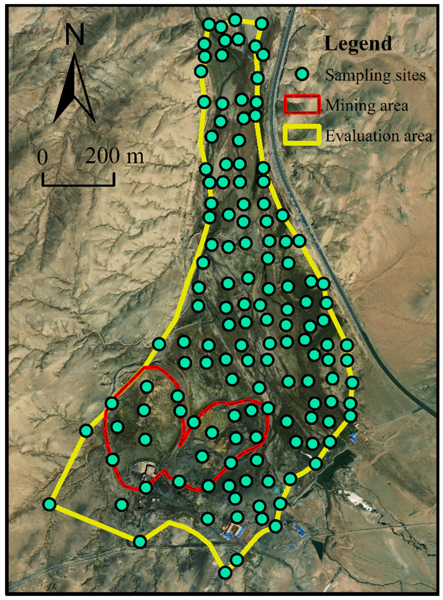
2.1. Study Area

The study area was located in Bayannur, Inner Mongolia Autonomous Region, at latitude 40°40′–42°22′ N and longitude 105°14′–107°36′ E. The area was once a natural grazing area, but at the end of the 20th century it became the copper flotation area of the Xinxing Copper Mine. Previous investigations have shown that beneficiation using copper sulfide and copper oxide as raw materials and the relevant processes involve grinding, classification, slurry mixing, and flotation (roughing, cleaning, and scavenging), etc., have caused heavy metal pollution of the surrounding areas.

2.2. Sample Collection and Treatment

Soil sampling was conducted with the requirements of the Technical Specification for Soil Environmental Monitoring (HJ/T 166-2004) and related specification documents [32]. The sampling sites are shown in Figure 1. The surface soil was collected after removing debris and vegetation by shovel, then, the soil under-surface was collected using a soil auger. Two samples of each different soil layer were taken at each point (soil layers at 0–10 cm, 10–30 cm, and 30–50 cm were recorded as S1, S2, and S3, respectively).

The soil samples were packed in marked plastic bags, sealed, stored away from light, and brought back to the laboratory for testing. Before testing these samples, the processing procedures were as follows: the soil samples were dried naturally; plant roots, rocks, and other impurities were picked out; and 0.1000 ± 0.0010 g samples were accurately weighed after passing through a 20-mesh sieve. The other preparation work before testing was according to Aydin and Soylak (2007) [33]. The soil sample testing parameters included pH; EC; and the concentrations of Pb, As, Cd, Cr, Cu, and Zn, etc. The pH was determined using composite electrodes (HI8424, Hana (China) Co., Ltd., Shanghai, China). The electrical conductivity (EC) was measured using a conductivity meter (using a 1:5 soil:extractant ratio, CD-5021A, Asone Corporation, Osaka, Japan. The total content of such metals were determined using an axial view inductively coupled plasma spectrometer (SPECTRO ARCOS, SPECTRO Analytical Instruments, Kleve, Germany). Detection limits for Cu, Zn, As, Pb, Cr, and Cd were 0.010 mg/kg, 0.010 mg/kg, 0.010 mg/kg, 0.005 mg/kg, 0.010 mg/kg, and 0.005 mg/kg, respectively.

2.3. Methods of Pollution Assessment

2.3.1. Pollution Index

The single factor index was used to evaluate the pollution degree of the soil. The calculation formula was as follows:

$$P_i{}^0=C_i / S_i$$

(1)

where P_i⁰ is the pollution index of number i pollutant in soil; C_i is the measured concentration of the number i pollutant, mg/kg; and S_i is the evaluation standard of number i pollutant, mg/kg, selected the screening values of the agricultural-land soil.

For each site with multiple pollutants in the study area, the maximum value of P_i calculated by various pollutants was chosen as the evaluation value.

$$P_i=\max \left(P_i{}^0\right)$$

(2)

2.3.2. Geological Accumulation Index

The geological accumulation index (I_geo), also known as the Muller index, and is a parameter to determine the degree of pollution by calculating the ratio between measured concentration value and background value of the pollutant [34]. It is described below:

$$I_{geo}{=Log}_2\left(\frac{C_i}{\lambda B_i}\right)$$

(3)

where C_i represents the detection concentration value of the number i heavy metal; B_i represents the background value of the number i heavy metal; and $\lambda$ is the correction coefficient, usually equal to 1.5.

2.3.3. The Nemerow Index

The Nemerow index (P_n) is widely applied to assess the level of the water or soil pollution. It was first proposed by Professor N.L. Nemerow. The P_n can be calculated by the following equations:

$$P_n=\sqrt{0.5\times (P_{\mathit{ave}}^2+P_{\mathit{max}}^2)}$$

(4)

$$P_{ave}=\frac{1}{n}{\displaystyle \sum _{i=1}^n{P}_i}$$

(5)

$$P_{\mathit{max}}=\max \{p_1,p_2,p_3\dots p_n\}$$

(6)

where P_max represents the maximum value of pollution index, P_ave represents the average value of the pollution index corresponding to each evaluation factors, P_i represents each pollution index of the evaluation factors, and n represents the number of different evaluation factors.

This index greatly amplifies the effect of the pollutant that seriously exceeds the standard, in order to avoid such a subversive impact of a single factor on the evaluation results, and thus more objectively and reasonably reflect the pollution risk generated by the comprehensive influence of various pollution factors in the evaluation area. A modified method based on the traditional Nemerow index method has emerged. Its formula is as follows:

$$P_n=\sqrt{0.5\times (P_{{}_{ave}}^2+P_c^2)}$$

(7)

$$P_c=0.5\times (P_{\mathit{max}}+P_w)$$

(8)

where, P_c refers to the maximum value of pollution index, and P_w is the pollution index of the factor with the highest weight in the improved evaluation system [35]. The weight of different factors in the modified Nemerow index is calculated as follows:

$$W_i=\frac{N_i}{{\displaystyle \sum _{i=1}^n{N}_i}}$$

(9)

$$N_i=\frac{L_{o\mathit{max}}}{L_{oi}},L_{o\mathit{max}}=\{L_{o1},L_{o2},L_{o3}\dots L_{on}\}$$

(10)

where L_Oi represents the standard value of each factor, N_i is the correlation, and W_i is the weight of each evaluation factor after normalization.

2.3.4. Ecological Risk Index

The ecological risk index (ER) was first introduced by Hakanson (1980) [36]. It can combine contaminant content, ecological effects, environmental effects, and toxicology to classify the potential ecological hazard level of heavy metals from a sedimentological perspective [37,38]. It is calculated as follows:

$$ER={\displaystyle \sum _{i=0}^n{E}_r^i}$$

(11)

$$E_r^i=T_r^i\times C_f^i$$

(12)

$$C_f^i=\frac{C_i}{C_i^0}$$

(13)

where, $C_f^i$ is the pollution index calculated by number i pollution factor, $C_i$ is the measured content of Cu/Zn/As/Pb/Cr/Cd, $C_i^0$ is the soil environmental background value of corresponding heavy metals, $E_r^i$ is the potential ecological hazard index of heavy metal i, and $T_r^i$ is the toxicity response parameter of the number i heavy metal.

2.3.5. Health Risk Index

The health risk index represents the possibility of human health damage in the presence of pollutants. A toxic or hazardous substance must reach a minimum dose (i.e., threshold) before it causes harm to the human body [39]. It can expressed using the hazard quotient (HQ), which is the ratio of the average daily human exposure dose (ADD, mg/kg/day) to the reference dose (R_fD, mg/kg/day).

$$AD{D}_i=\frac{C\times IR\times EF\times ED}{B{W}_{\mathrm{a}}\times AT}$$

(14)

$$H{Q}_i=\frac{AD{D}_i}{R_f{D}_i}\times {10}^{-6}$$

(15)

$$HI={\displaystyle \sum _{i=1}^{n}H{Q}_i}$$

(16)

where ADD_i refers to the daily average exposure of pollutants, mg/(kg∙d); C is the concentration of pollutants in soil, mg/kg; IR means daily average intake of soil, mg/d; EF is exposure frequency, d/a; ED is the continuous exposure, a; AT is the average exposure time, D; BWA is body weight (adult), kg; HQ_i is the exposure risk from single factor; and HI is the total exposure risk index under the action of multiple heavy metals [40].

2.4. Methods of Pollution Assessment

SPSS 20 software (SPSS Inc., Chicago, IL, USA) was used for data verification. The Grubbs test was used (significance level was set at 0.05) to eliminate outliers. Analysis of variance (significance level was set at 0.05) was to confirm whether the data had statistical significance (p < 0.05).

According to the environment characteristics of the Xinxing copper mine and its influencing area, the study area conforms to the agricultural land standards stipulated in the Classification of Land Use Status (GB/T 21010) [41], and belongs to the natural grassland, then based on Soil Environment Quality Risk Control Standard for Soil Contamination of Agriculture Land (GB 15618-2018) [42], which has been officially implemented since 1 August 2018. We obtained the control standard for soil heavy-metal contamination, which is shown in

Table 1. Soil environment quality risk control standards (mg/kg).

Standard Items	pH	Cu	Zn	As	Pb	Cr	Cd
Risk screening values	pH ≤ 5.5	50	200	40	70	150	0.3
	5.5 < pH ≤6.5	50	200	40	90	150	0.3
	6.5 < pH ≤7.5	100	250	35	120	200	0.3
	7.5 < pH	100	300	25	170	250	0.6
Risk intervention values	pH ≤ 5.5	-	-	200	400	800	1.5
	5.5 < pH ≤ 6.5	-	-	150	500	850	2.0
	6.5 < pH ≤ 7.5	-	-	120	700	1000	3.0
	7.5 < pH	-	-	100	1000	1300	4.0

Note: “-” means not given.

.

The evaluation results were spatially interpolated using Surfer 15, and the relevant data were fed into the two-dimensional plane. In the meantime the evaluation area boundary file was created. We chose this area to analyze the risk level of soil heavy-metal pollution and to obtain a distribution map of soil heavy-metal risk levels. Then, the grid data of different risk areas were analyzed by using ArcGIS 10.7 (Esri, Inc., Redlands, CA, USA) vectorization function to obtain the risk levels of different soil areas.

3. Results

3.1. Descriptive Statistics of Heavy Metal Concentrate in Soil

Based on the test result of soil samples, the heavy metal concentrations in the study area were analyzed in detail. As shown in

Table 2. Test results of soil heavy metals in the study area.

Metals	Layers	Max (mg/kg)	Min (mg/kg)	Median (mg/kg)	Mean (mg/kg)	SD	CV (%)
Cu	S1	2954	12	131	272	362.39	133.39
	S2	1917	5	76	189	292.19	154.21
	S3	1122	4	53	151	224.09	148.35
Zn	S1	350	16	82	102	57.69	56.45
	S2	355	9	67	86	56.13	65.41
	S3	282	8	65	76	44.64	58.42
As	S1	89	0.2	12	18	15.45	84.57
	S2	139	0.3	10	13	13.42	104.86
	S3	85	0.1	10	12	11.74	95.10
Pb	S1	1134	6	53	103	130.07	126.72
	S2	1945	4	41	97	205.36	211.35
	S3	821	1	39	66	98.37	149.63
Cr	S1	193	12	53	56	23.38	42.11
	S2	187	13	60	58	25.26	43.21
	S3	121	15	54	55	22.69	40.99
Cd	S1	1.60	0.05	0.20	0.25	0.18	69.80
	S2	1.08	0.03	0.18	0.24	0.18	77.03
	S3	1.12	0.03	0.16	0.22	0.17	77.57

Note: Max = maximum value, Min = minimum value, Median = median value, SD = standard deviation, CV = coefficient of variation.

, the average Cu concentration in the soil samples was 204.07 mg/kg, with a standard deviation of 302.73; the concentration values between 3.77 and 751.60 mg/kg accounted for 95% of all the samples. The average Zn concentration was 88.15 mg/kg, with a standard deviation of 54.24. The samples with concentration values between 8.46 and 202.80 mg/kg accounted for 95% of all the samples. The average concentration of As was 14.47 mg/kg, and the standard deviation was 13.90. The samples with concentration values between 0.13 and 38.85 mg/kg accounted for 95% of all the samples. The average Pb concentration was 88.52 mg/kg, with a standard deviation of 152.39. The samples with concentration values between 1.04 and 275.00 mg/kg accounted for 95% of all the samples. The average value of Cr concentration in the site soil was 56.45 mg/kg, and the standard deviation was 23.86. The samples with concentration values between 11.60 and 93.49 mg/kg accounted for 95% of all the samples. The average Cd concentration was 0.235 mg/kg, with a standard deviation of 0.176. The samples with concentration values between 0.028 and 0.581 mg/kg accounted for 95% of all the samples.

The pH values were between 2.870 and 9.195, 2.505 and 9.035, and 2.245 and 9.645 for S1, S2, and S3, respectively, and the average values were 7.965, 7.996, and 8.079, respectively. The EC values were between 0.034 and 24310 us/cm, 51.28 and 9703 us/cm, and 59.48 and 11050 us/cm for S1, S2, and S3, respectively, and the average values were 3638.966, 1904.617, and 1636.660, respectively.

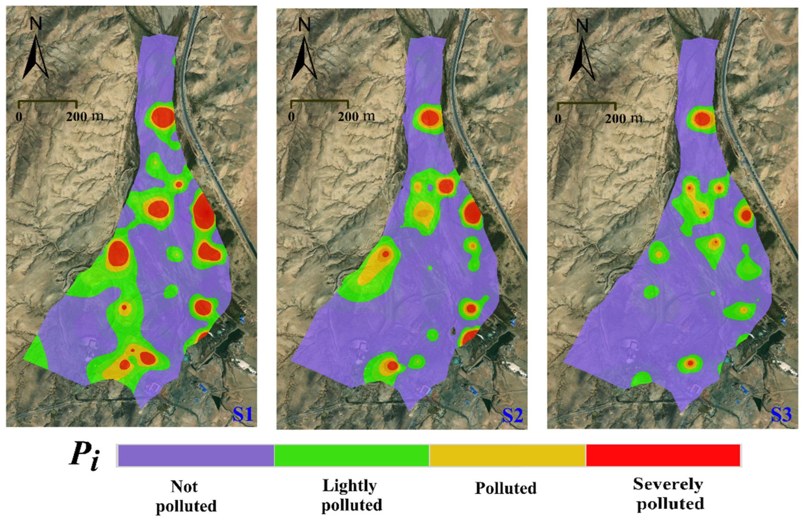
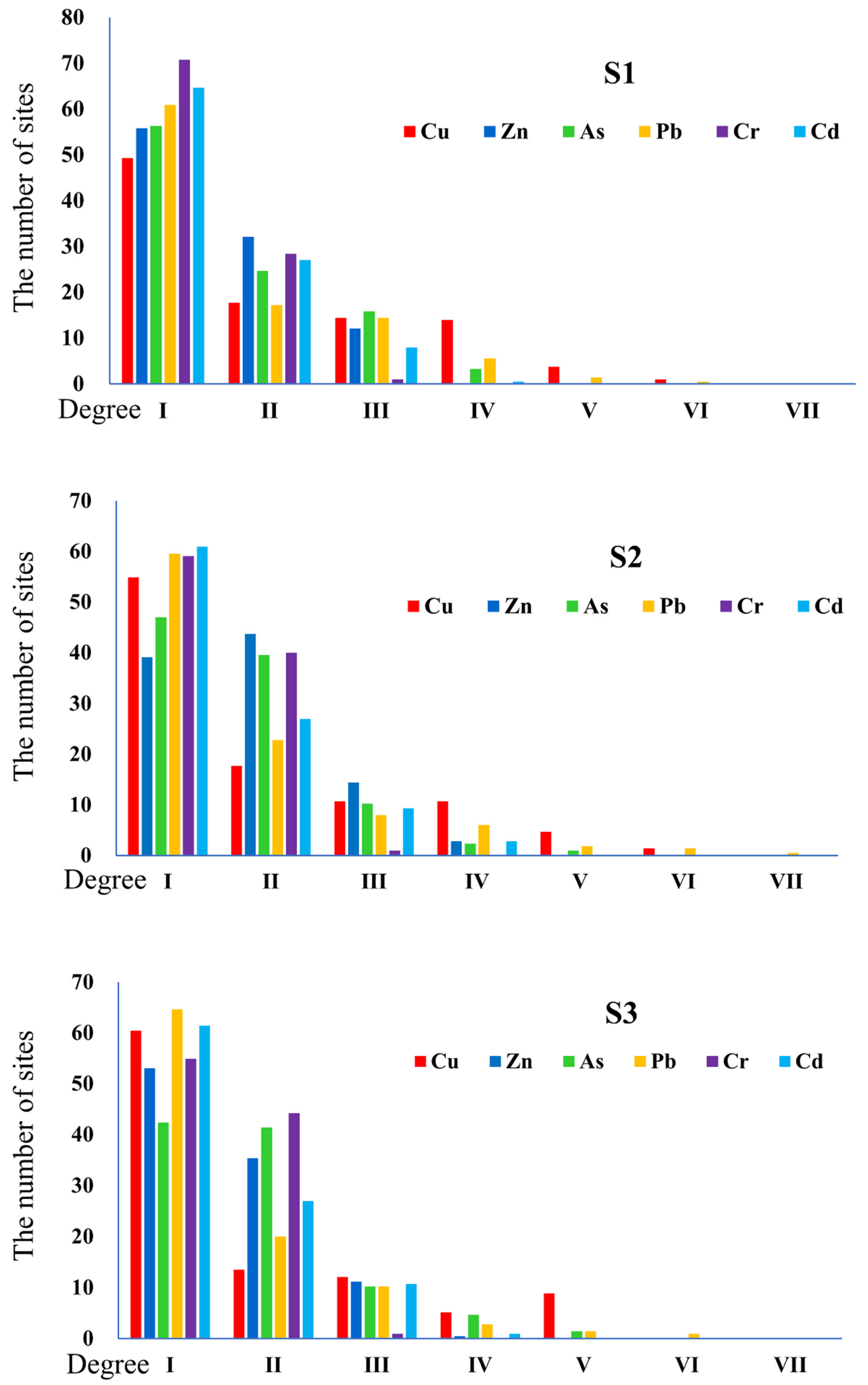
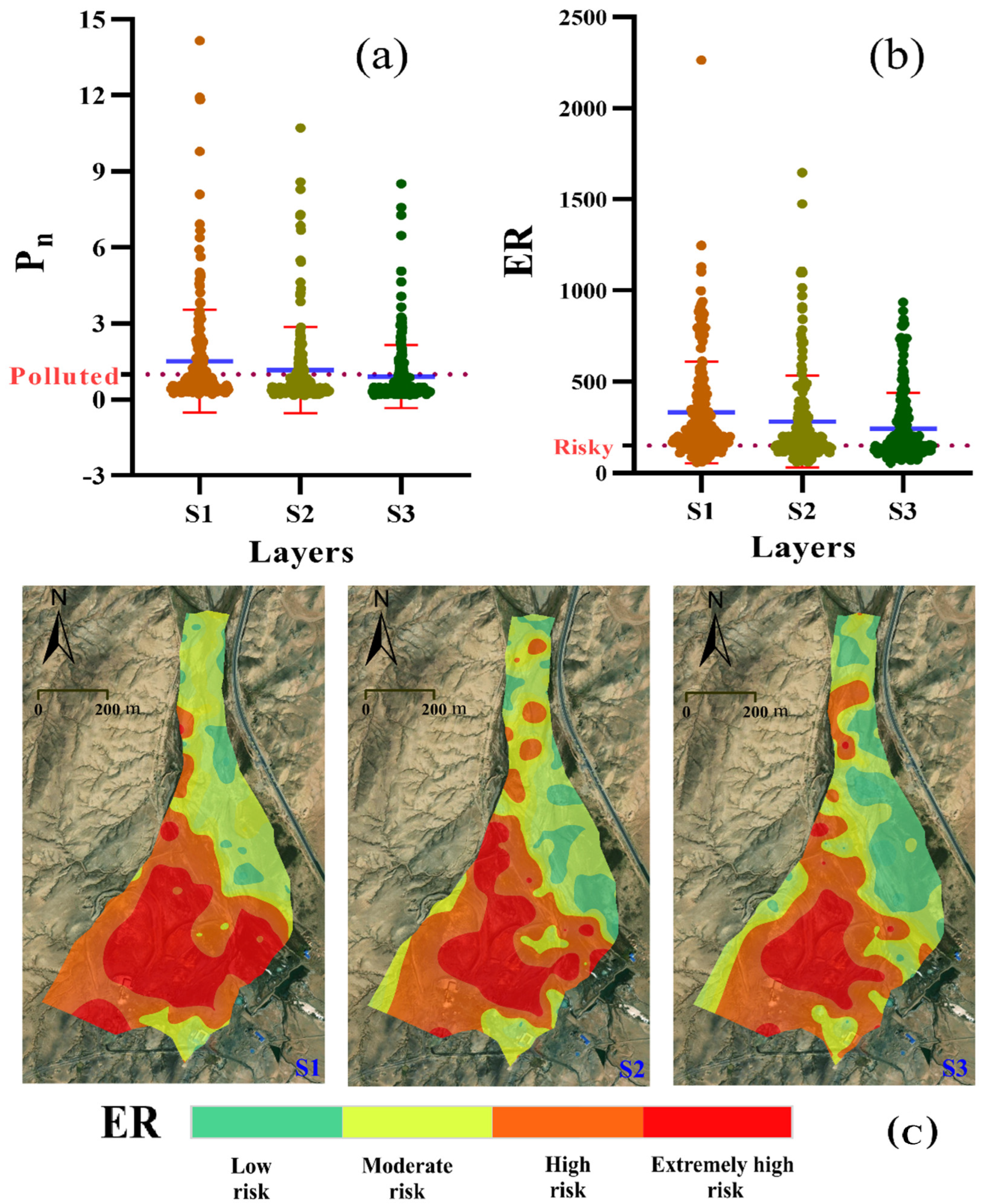
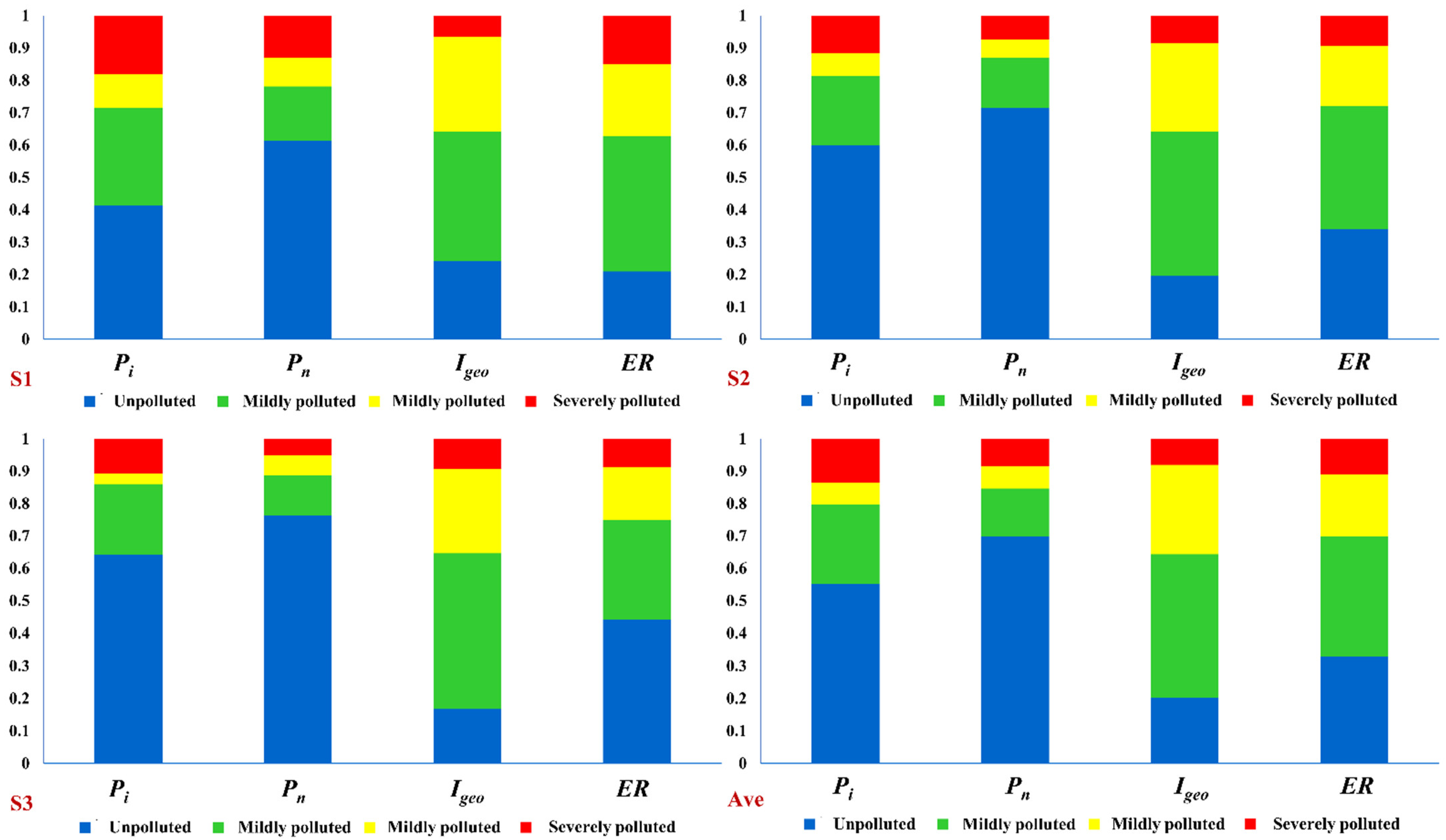
3.2. Evaluation Results of Different Indices

The evaluation results of a single factor index were divided into four levels from high to low, according to the P_i value: severely polluted (>5), polluted (3–5), lightly polluted (1–3), and not polluted (<1).

Based on the results of single-factor index evaluation, the distribution of the severely polluted points evaluated by the single-factor index were more dispersed under the action of different pollution factors (Figure 2). In the 0–10 cm soil layer, 41.40% of the sampling points were at non-pollution level, while the number of severely polluted points accounted for nearly one fifth. This proportion changed with the increase in soil depth—in the 10–30 cm soil layer, the number of points at a non-pollution level increased significantly to 60.00%, while the number of the soil points at severe-pollution level decreased to 11.63%. With further increase in soil depth, the number of pollutant points also changed, but the magnitude of change slowed down. The same situation also occurred with heavy pollution—compared to the surface soil, in the 30–50 cm soil layer the proportion of non-pollution points rose by 22.79% and the number of points with heavy pollution decreased by 7.44%. The changes in the evaluation results of the first and second soil layers far exceeded the changes in the second and third soil layers.

We selected 15 points within two kilometers of the study area as the background-value sampling points, and standardized methods were used for data processing. Taking the average concentration of heavy metals in different soil layers as the background value (

Table 3. Background values of soil heavy metals in the study area (mg/kg).

Soil Layers	Cu	Zn	As	Pb	Cr	Cd
S1	101.89	78.44	12.42	58.37	57.94	0.23
S2	75.18	54.54	8.83	44.84	57.69	0.19
S3	63.98	60.52	7.33	42.18	50.66	0.17

), according the standard of the geological accumulation index method, I_geo < 0 indicated no pollution (the pollution degree was I); 0 ≤ I_geo < 1 indicating light to moderate pollution (the pollution degree was II); 1 ≤ I_geo < 2 indicating moderate pollution (the pollution degree was III); 2 ≤ I_geo < 3 indicating medium-high pollution (the pollution degree was IV); 3 ≤ I_geo < 4 indicating high pollution (the pollution degree was V); 4 ≤ I_geo < 5 indicating high-extreme pollution (the pollution degree was VI); and I_geo ≥ 5 indicating extreme pollution (the pollution degree was VII).

On the whole, using I_geo to evaluate the risk of heavy metals in the soils of the study area, most of the points had no pollution (Figure 3), with only a small number of points having moderate pollution or a more serious level of pollution. Comparing the evaluation results of pollution levels of different soil layers, showed that the number of non-pollution points in the study area decreased with increase in soil depth, which was mainly due to the fact that the decrease in soil heavy-metal background values with increasing soil depth was greater than the decrease in heavy metal concentrations with increasing soil depth in the copper-mine-impacted area. The low background value of heavy metals in deep soils can be used to disturb the deep-soil environment through vertical migration for the more migratory heavy metal contaminants. Thus, this index focuses more on reflecting the dynamic change results of pollutant content in the evaluation area rather than the pollutant content level itself.

The evaluation results of the Nemerow index method are shown in Figure 4a. The maximum and minimum values of P_n for the 0–10 cm, 10–30 cm, and 30–50 cm soil layers were 14.15 and 0.21, 10.72 and 0.16, and 8.51 and 0.17, respectively, which corresponded to the risk level of highly contaminated and clean.

With increase in soil depth, the potential ecological risk of heavy metals in the study area decreased continuously and the sites with medium ecological risk, high ecological risk, and very high ecological risk all decreased to a certain extent (Figure 4b). Conversely, the proportion of soil sites with low ecological risk level increased—79.07% of the sites in the 0–10 cm soil layer were in the medium ecological risk level or above, with the highest RI value being 2263.45, and the lowest being 57.96. The highest ER value was 2263.45 and the lowest was 57.96; 66.05% of the sites in the 10–30 cm soil layer were at medium ecological risk or above, with a maximum ER value of 1647.45 and a minimum value of 59.24, while only 55.81% of the sites in the 30–50 cm soil layer were at medium or higher ecological risk (Figure 4c).

Considering the actual study area situation, we used the exposure risk (non-carcinogenic risk) to characterize the human health risk. Referring to the guidance document of USPA [43], the maximum and minimum values of HI in the 0–10 cm, 10–30 cm, and 30–50 cm soil layers were 6.35 0.45, and 7.60 and 0.35, 5.87, and 0.45, respectively, with mean values of 1.94, 1.76, and1.61, respectively. As shown in Figure 5, 14.42%, 19.53%, and 22.33% of the area was maintained at the no-risk level in the three soil layers from shallow to deep, and the rest was at the low-risk level. All soil sites were at limited risk without the evaluation result of high non-carcinogenic health risk. In general, the human health risk in this area was low.

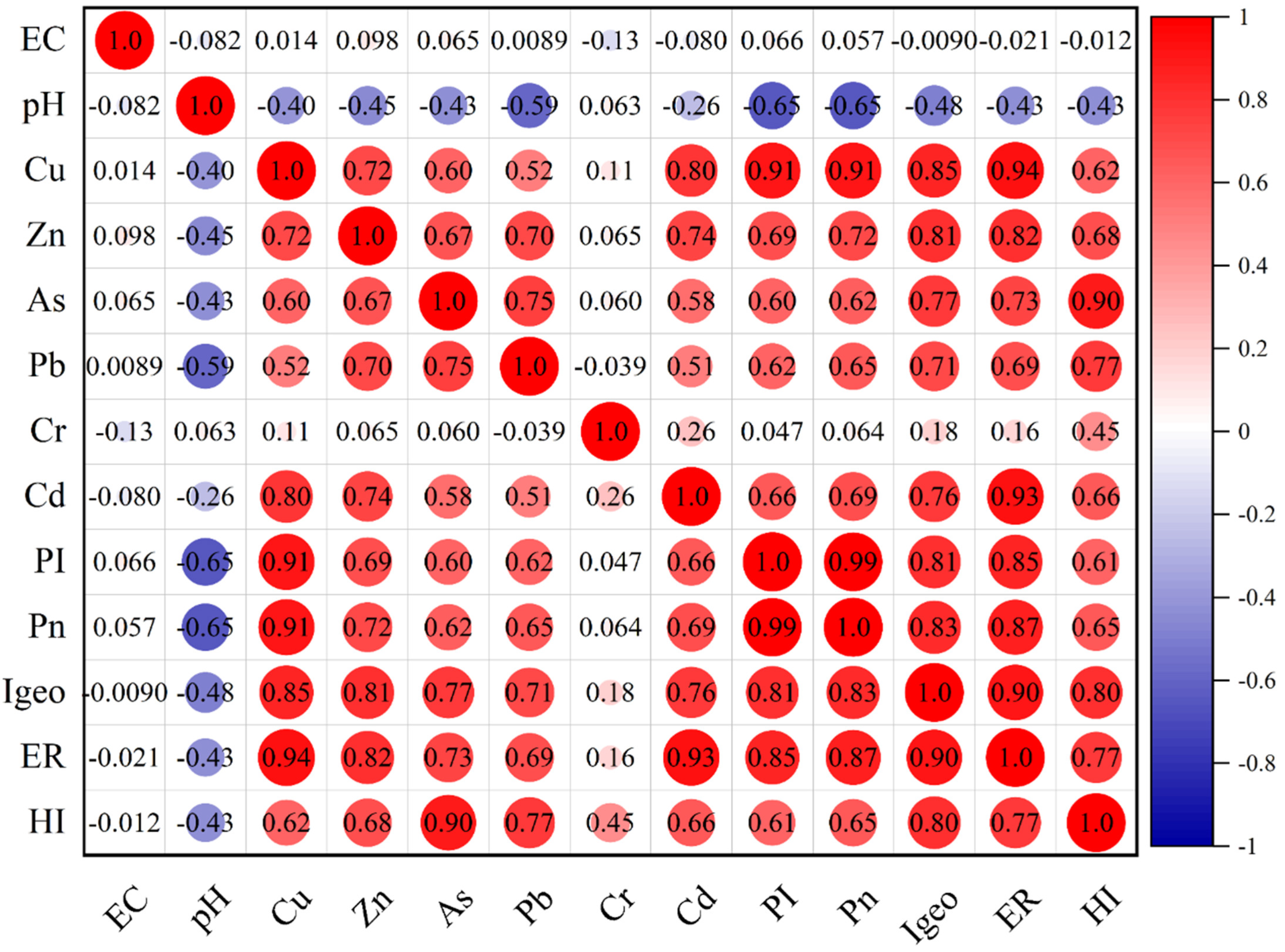
3.3. Comparison of Different Evaluation Indices

Taking the average values of several parallel samples, correlation analysis was carried out for different detected parameters as well as for the evaluation indices. As shown in Figure 6, except for Cr, various heavy metals showed significant correlation with the calculated values of different indices, among which the correlation between the Cu and other heavy metals was prominent, with the correlation coefficients of 0.91, 0.91, 0.85, and 0.94 with P_i, P_n, I_geo, and ER, respectively, while the correlation coefficient with HI was relatively low at 0.62.

For the different indices, the evaluation values generally showed a positive correlation, especially between P_i and P_n, with a correlation coefficient as high as 0.99. The correlation between I_geo and ER was also prominent with a correlation coefficient of 0.9. In addition, the results of different evaluation indices had high correlation, but this was relatively limited. For example, the correlation coefficient between HI, P_i and P_n was at a low level, and there were different degrees of variability and uncertainty of evaluation results between different indices.

Different indices have different emphases when applied to the soil pollution assessment, and there are great gaps among them. Taking P_i, P_n, I_geo, ER, for example, and reclassifying all evaluation results into four degrees, “unpolluted”, “mildly polluted”, “moderately polluted”, and “severely polluted”, the “no pollution” in the evaluation result of I_geo and the “light–severe pollution” are regarded as “unpolluted”; the degrees of “moderate pollution” and “medium–high pollution” are regarded as “moderately polluted”; the “high pollution”, “high–extreme pollution”, and “extreme pollution” are regarded as “severely polluted”. The original four risk levels for ER correspond to “unpolluted”, “mildly polluted”, “moderately polluted”, and “severely polluted”. In order to determine the area occupied by different evaluation results, ArcGIS was used to measure the area by geostatistical methods. First, the file of the evaluation area boundary was read and recorded directly. The area was found to be 440,005.66 m². A contour map rasterized in the China Geodetic Coordinate System 2000 (CGCS2000) coordinate system was then drawn, and the interpolated values of each raster in the area were obtained by rasterization and calculation, the dates were exported to Excel, and the number of interpolated values in different contamination degrees was counted and divided by the total number of raster points to get the proportion of the area of different pollution levels under each applied index, as shown in Figure 7.

For the 0–10 cm soil layer, the evaluation result of P_n had the most points in the risk level of “unpolluted”, accounting for 61.36%, while the ER had the lowest percentage, accounting for only 20.93%. The former proportion was about three times that of the latter, while the proportion of the points for P_n and ER at the “severely polluted” level was 13.02% and 18.89%, respectively, at the high-pollution-risk level. This difference was not significant. The proportion of “severely polluted” points in the evaluation result of P_i was relatively high compared with other methods, reaching 18.14%, and the lowest proportion of “severely polluted” points evaluated by I_geo was only 6.51%. The results of the ER showed that the highest percentage of “mildly polluted” was 41.86% and the lowest percentage of “severely polluted” was 14.88% in the top layer of the study area. For the 10–30 cm soil layer, the sampling points with highest percentage evaluated as “severely polluted” was still by the P_i (11.63%), followed by ER (9.30%), and the lowest by the P_n (7.44%). The P_n brought the highest percentage of “unpolluted” points in the surface soil, and the lowest was the I_geo, with the proportions of 71.63% and 24.19%, respectively. With further increase in soil depth, the number of points at the “unpolluted” level for each index increased, among which the P_n reached 76.28% and the lowest was the I_geo, with the percentage of “unpolluted” points being 16.74%. The number of “unpolluted” and “mildly polluted” sites in the 30–50 cm soil layer was higher—44.19% and 30.70%, respectively, while the percentage of “severely polluted” sites was higher. The percentage of sites at “unpolluted” and “mildly polluted” levels in the 30–50 cm soil layer was 44.19% and 30.70%, respectively, while the percentage of “severely polluted” sites was only 8.84%. In the 30–50 cm soil layer, the highest and lowest percentages of “severely polluted” were still evaluated by P_n, with percentages of 10.70% and 5.12%, respectively.

4. Discussion

Among the multiple metals detected in the study area, Cu, Zn, As, Pb, Cr, and Cd all have adverse effects on human health when exposures exceed the tolerable dose levels. The percentage of sampling points for Cu exceeding the screening value was the highest, with 57.21%, 39.07%, and 33.95% sites in the three soil layers in S1, S2, and S3. Pb and As in the surface soil also exceeded the screening values, with 19.53% and 18.14%, respectively. Comparison between the detection and screening values of Cr showed that there was no Cr contamination in any soil-sampling sites in the study area. There was a clear correlation between soil depth and screening results, with the number of sites exceeding screening values for Cu, Zn, As, and Pb decreasing with increasing soil depth, while Cd showed a similar number of soil contents exceeding screening values in the second and third layers, but there was a significant decrease compared to the surface soil. In addition, pH also had an influence on the results of soil heavy-metal pollution-risk screening. As, due to the toxicity of acidic conditions is neutralized by ions, leading to relatively low limit values. Therefore, the second layer of soil did not exceed the standard. Moreover, 9.77% of the surface-soil samples had Cd levels between the screening and control values, which, according to GB 15618-2018, means that the site is at risk of soil contamination and should be monitored. Pb was the only measured heavy metal that exceeded the control value, and the number of points above the control value for the three layers of soil were 4, 5, and 3, in order, from shallow to deep. Although soil environment quality risk control standards serve as the official system for evaluating soil quality, they are not very useful in practice because they are each for only for one metal, and no clear guidelines are given for the synergistic effect of multiple pollutants. Therefore, the evaluation of different indices based on these standards has a large value space.

According to the comparison of the evaluation results, the emphasis of the different indices differs, with P_i emphasizing the reliance on the most dominant pollution factor and the modified P_n effectively diminishing the decisive role of this major pollution metal on the evaluation results. The I_geo is a tool similar to the enrichment factor, and it always depends on the difference between the measured concentration and the soil heavy-metal background values. The ER can narrow the gap between soil heavy-metal pollution and biological health risks and evaluate the potential ecological hazards of soil pollution, and HI provide a scientific reference for human health. Therefore, it is necessary to carry out a comprehensive evaluation system of soil contamination risk in typical tailing areas and take corresponding measures for contaminated soil of different risk levels. In this way we can effectively control regional soil ecological risks and provide condition-friendly land for agricultural and human activities in mining areas.

5. Conclusions

Through the detection and analysis of soil heavy-metal concentrations in the affected area of the Xinxing Copper Mine in the Inner Mongolia Autonomous Region, and comparison with the national standards, it was found that the content of heavy metals Cu and Pb in many sites exceeded the national standards—the peak value of Cu content exceeded the national standards by 37 times and the peak value of Pb exceeded the national standards by 19 times. It was also found that with the increase of soil depth, the content of heavy metals except Cr decreased significantly, and a large number of heavy metals were enriched in the surface or shallow soil.

Moreover, multiple indices were applied to distinguish the pollution risk, and it was found that the evaluation results were significantly different under different indices. Comparing the results of different evaluation indices, it was concluded that, overall, P_i occupies a higher risk level than other methods, such as the I_geo or the modified P_n. On the other hand, P_n weakens the dominant role of the main pollution factor (Cu), while leaving more areas at a safe degree of contamination risk, a result that needs to be alerted to in order to avoid over-optimism in further soil-pollution treatment and land management. Additionally, it is better to adopt appropriate pollution risk indices according to the situation of the assessment area, such as heavy metal background value and land type. Of course, a scientific and reasonably comprehensive evaluation system is also worth looking forward to.

References

1. Solgi, E.; Esmaili-Sari, A.; Riyahi-Bakhtiari, A.; Hadipour, M. Soil Contamination of Metals in the Three Industrial Estates, Arak, Iran. Bull. Environ. Contam. Toxicol. 2012, 88, 634–638. [Google Scholar] [CrossRef] [PubMed]
2. Zhao, X.; Huang, J.; Lu, J.; Sun, Y. Study on the influence of soil microbial community on the long-term heavy metal pollution of different land use types and depth layers in mine. Ecotoxicol. Environ. Saf. 2019, 170, 218–226. [Google Scholar] [CrossRef] [PubMed]
3. Liu, B.; Ai, S.; Zhang, W.; Huang, D.; Zhang, Y. Assessment of the bioavailability, bioaccessibility and transfer of heavy metals in the soil-grain-human systems near a mining and smelting area in NW China. Sci. Total Environ. 2017, 609, 822–829. [Google Scholar] [CrossRef] [PubMed]
4. Jamshidi-Zanjani, A.; Saeedi, M. Multivariate analysis and geochemical approach for assessment of metal pollution state in sediment cores. Environ. Sci. Pollut. Res. 2017, 24, 16289–16304. [Google Scholar] [CrossRef] [PubMed]
5. Arabyarmohammadi, H.; Darban, A.K.; Abdollahy, M.; Yong, R.; Ayati, B.; Zirakjou, A.; van der Zee, S.E.A.T. Utilization of a Novel Chitosan/Clay/Biochar Nanobiocomposite for Immobilization of Heavy Metals in Acid Soil Environment. J. Polym. Environ. 2018, 26, 2107–2119. [Google Scholar] [CrossRef]
6. Lashen, Z.M.; Shams, M.S.; El-Sheshtawy, H.S.; Slany, M.; Antoniadis, V.; Yang, X.; Sharma, G.; Rinklebe, J.; Shaheen, S.M.; Elmahdy, S.M. Remediation of Cd and Cu contaminated water and soil using novel nanomaterials derived from sugar beet processing- and clay brick factory-solid wastes. J. Hazard. Mater. 2022, 428, 128205. [Google Scholar] [CrossRef]
7. Zhang, X.; Yang, H.; Cui, Z. Evaluation and analysis of soil migration and distribution characteristics of heavy metals in iron tailings. J. Clean. Prod. 2018, 172, 475–480. [Google Scholar] [CrossRef]
8. Huang, J.; Guo, S.; Zeng, G.; Li, F.; Gu, Y.; Shi, Y.; Shi, L.; Liu, W.; Peng, S. A new exploration of health risk assessment quantification from sources of soil heavy metals under different land use. Environ. Pollut. 2018, 243, 49–58. [Google Scholar] [CrossRef]
9. Patra, D.K.; Acharya, S.; Pradhan, C.; Patra, H.K. Poaceae plants as potential phytoremediators of heavy metals and eco-restoration in contaminated mining sites. Environ. Technol. Innov. 2021, 21, 101293. [Google Scholar] [CrossRef]
10. Shahsavari, A.; Yazdi, F.T.; Moosavi, Z.; Heidari, A.; Sardari, P. A study on the concentration of heavy metals and histopathological changes in Persian jirds (Mammals; Rodentia), affected by mining activities in an iron ore mine in Iran. Environ. Sci. Pollut. Res. Int. 2019, 26, 12590–12604. [Google Scholar] [CrossRef]
11. Hanfi, M.Y.; Mostafa, M.Y.A.; Zhukovsky, M.V. Heavy metal contamination in urban surface sediments: Sources, distribution, contamination control, and remediation. Environ. Monit. Assess. 2019, 192, 32. [Google Scholar] [CrossRef] [PubMed]
12. Nanos, N.; Rodriguez Martin, J.A. Multiscale analysis of heavy metal contents in soils: Spatial variability in the Duero river basin (Spain). Geoderma 2012, 189–190, 554–562. [Google Scholar] [CrossRef]
13. Zhai, L.; Liao, X.; Chen, T.; Yan, X.; Xie, H.; Wu, B.; Wang, L. Regional assessment of cadmium pollution in agricultural lands and the potential health risk related to intensive mining activities: A case study in Chenzhou City, China. J. Environ. Sci. 2008, 20, 696–703. [Google Scholar] [CrossRef]
14. Wu, S.; Peng, S.; Zhang, X.; Wu, D.; Luo, W.; Zhang, T.; Zhou, S.; Yang, G.; Wan, H.; Wu, L. Levels and health risk assessments of heavy metals in urban soils in Dongguan, China. J. Geochem. Explor. 2015, 148, 71–78. [Google Scholar] [CrossRef]
15. Teng, Y.; Wu, J.; Lu, S.; Wang, Y.; Jiao, X.; Song, L. Soil and soil environmental quality monitoring in China: A review. Environ. Int. 2014, 69, 177–199. [Google Scholar] [CrossRef] [PubMed]
16. Lv, J. Multivariate receptor models and robust geostatistics to estimate source apportionment of heavy metals in soils. Environ. Pollut. 2019, 244, 72–83. [Google Scholar] [CrossRef]
17. Zhang, Q.; Wang, C. Natural and Human Factors Affect the Distribution of Soil Heavy Metal Pollution: A Review. Water Air Soil Pollut. 2020, 231, 350. [Google Scholar] [CrossRef]
18. Antoniadis, V.; Shaheen, S.M.; Boersch, J.; Boersch, J.; Frohne, T.; Du Laing, G.; Rinklebe, J. Bioavailability and risk assessment of potentially toxic elements in garden edible vegetables and soils around a highly contaminated former mining area in Germany. J. Environ. Manag. 2017, 186, 192–200. [Google Scholar] [CrossRef]
19. Yang, S.; Zhou, D.; Yu, H.; Wei, R.; Pan, B. Distribution and speciation of metals (Cu, Zn, Cd, and Pb) in agricultural and non-agricultural soils near a stream upriver from the Pearl River, China. Environ. Pollut. 2013, 177, 64–70. [Google Scholar] [CrossRef]
20. Acosta, J.A.; Jansen, B.; Kalbitz, K.; Faz, A.; Martinez-Martinez, S. Salinity increases mobility of heavy metals in soils. Chemosphere 2011, 85, 1318–1324. [Google Scholar] [CrossRef]
21. Cerqueira, B.; Covelo, E.F.; Andrade, L.; Vega, F.A. The influence of soil properties on the individual and competitive sorption and desorption of Cu and Cd. Geoderma 2011, 162, 20–26. [Google Scholar] [CrossRef]
22. Hu, Z.; Wang, C.; Li, K.; Zhu, X. Distribution characteristics and pollution assessment of soil heavy metals over a typical nonferrous metal mine area in Chifeng, Inner Mongolia, China. Environ. Earth Sci. 2018, 77, 638. [Google Scholar] [CrossRef]
23. Costa, M.; Henriques, B.; Pinto, J.; Fabre, E.; Viana, T.; Ferreira, N.; Amaral, J.; Vale, C.; Pinheiro-Torres, J.; Pereira, E. Influence of salinity and rare earth elements on simultaneous removal of Cd, Cr, Cu, Hg, Ni and Pb from contaminated waters by living macroalgae. Environ. Pollut. 2020, 266, 1153741. [Google Scholar] [CrossRef]
24. Gong, Q.; Deng, J.; Xiang, Y.; Wang, Q.; Yang, L. Calculating pollution indices by heavy metals in ecological geochemistry assessment and a case study in parks of Beijing. J. China Univ. Geosci. 2008, 19, 230–241. [Google Scholar]
25. Tan, K.; Ma, W.; Chen, L.; Wang, H.; Du, Q.; Du, P.; Yan, B.; Liu, R.; Li, H. Estimating the distribution trend of soil heavy metals in mining area from HyMap airborne hyperspectral imagery based on ensemble learning. J. Hazard. Mater. 2021, 401, 123288. [Google Scholar] [CrossRef]
26. Mazurek, R.; Kowalska, J.; Gasiorek, M.; Zadrozny, P.; Jozefowska, A.; Zaleski, T.; Kepka, W.; Tymczuk, M.; Orlowska, K. Assessment of heavy metals contamination in surface layers of Roztocze National Park forest soils (SE Poland) by indices of pollution. Chemosphere 2017, 168, 839–850. [Google Scholar] [CrossRef]
27. Zhang, H.M.; Zhang, H.; Song, A.; Qin, J.; Song, M. Evaluation of Ecological Risk on Soil Heavy Metals Pollution of Qingyuan. Prog. Environ. Sci. Eng. 2013, 610–613, 928–931. [Google Scholar] [CrossRef]
28. Liu, L.; Li, W.; Song, W.; Guo, M. Remediation techniques for heavy metal-contaminated soils: Principles and applicability. Sci. Total Environ. 2018, 633, 206–219. [Google Scholar] [CrossRef]
29. Li, S.; Wu, J.; Huo, Y.; Zhao, X.; Xue, L. Profiling multiple heavy metal contamination and bacterial communities surrounding an iron tailing pond in Northwest China. Sci. Total Environ. 2021, 752, 141827. [Google Scholar] [CrossRef]
30. Wang, S.; Kalkhajeh, Y.K.; Qin, Z.; Jiao, W. Spatial distribution and assessment of the human health risks of heavy metals in a retired petrochemical industrial area, south China. Environ. Res. 2020, 188, 109661. [Google Scholar] [CrossRef]
31. Christou, A.; Theologides, C.P.; Costa, C.; Kalavrouziotis, I.K.; Varnavas, S.P. Assessment of toxic heavy metals concentrations in soils and wild and cultivated plant species in Limni abandoned copper mining site, Cyprus. J. Geochem. Explor. 2017, 178, 16–22. [Google Scholar] [CrossRef]
32. HJ/T 166-2004; Technical Specification for Soil Environmental Monitoring. State Environmental Protection Administration (Ministry of Ecology and Environment of the People’s Republic of China): Beijing, China, 2004.
33. Aydin, F.A.; Soylak, M. A novel multi-element coprecipitation technique for separation and enrichment of metal ions in environmental samples. Talanta 2007, 73, 134–141. [Google Scholar] [CrossRef] [PubMed]
34. Muller, G. Index of geoaccumulation in sediments of the Rhineriver. Geojournal 1969, 2, 108. [Google Scholar]
35. Han, I.; Whitworth, K.W.; Christensen, B.; Afshar, M.; Han, H.A.; Rammah, A.; Oluwadairo, T.; Symanski, E. Heavy metal pollution of soils and risk assessment in Houston, Texas following Hurricane Harvey. Environ. Pollut. 2022, 296, 118717. [Google Scholar] [CrossRef]
36. Hakanson, L. An ecological risk index for aquatic pollution control: A sedimentological approach. Water Res. 1980, 14, 975–1001. [Google Scholar] [CrossRef]
37. Lu, S.; Wang, Y.; He, L. Ecological Risk of Heavy Metals on the Paddy Soils at a Village in Hunan. Enuivon. Sci. Technol. 2014, 37, 100–105, 117. [Google Scholar]
38. Deng, M.; Zhu, Y.; Shao, K.; Zhang, Q.; Ye, G.; Shen, J. Metals source apportionment in farmland soil and the prediction of metal transfer in the soil-rice-human chain. J. Environ. Manag. 2020, 260, 110092. [Google Scholar] [CrossRef]
39. Ben Chabchoubi, I.; Mtibaa, S.; Ksibi, M.; Hentati, O. Health risk assessment of heavy metals (Cu, Zn, and Mn) in wild oat grown in soils amended with sediment dredged from the Joumine Dam in Bizerte, Tunisia. Euro-Mediterr. J. Environ. Integr. 2020, 5, 60. [Google Scholar] [CrossRef]
40. Chonokhuu, S.; Batbold, C.; Chuluunpurev, B.; Battsengel, E.; Dorjsuren, B.; Byambaa, B. Contamination and Health Risk Assessment of Heavy Metals in the Soil of Major Cities in Mongolia. Int. J. Environ. Res. Public Health 2019, 16, 2552. [Google Scholar] [CrossRef] [Green Version]
41. GB/T21010-2017; Current Land Use Classification. General Administration of Quality Supervision, Inspection and Quarantine of the People’s Republic of China; Standardization Administration of the People’s Republic of China: Beijing, China, 2017.
42. GB-15618-2018; Soil Environment Quality Risk Control Standard for Soil Contamination of Agriculture Land. Ministry of Ecology and Environment of the People’s Republic of China; State Administration of Market Regulation: Beijing, China, 2018.
43. USEPA. Exposure Factors Handbook; General Factors; USEPA: Washington, DC, USA, 1996; Volume I.
Figure 1. Soil sampling sites in the evaluation area.
Minerals 12 01074 g001
Figure 2. Distribution of Pi-values in the study area. S1: 0–10 cm soil layer; S2: 10–30 cm soil layer; S3: 30–50 cm soil layer.
Minerals 12 01074 g002
Figure 3. The results of pollution degree base on Igeo. S1: 0–10 cm soil layer; S2: 10–30 cm soil layer; S3: 30–50 cm soil layer.
Minerals 12 01074 g003
Figure 4. Evaluation results of Pn and ER in different soil layers. (a): Evaluation results of the modified Nemerow index. (b): Evaluation results of the ecological risk index. (c): Distribution map of heavy metal ecological risk index in the evaluation area. S1: 0–10 cm soil layer; S2: 10–30 cm soil layer; S3: 30–50 cm soil layer.
Minerals 12 01074 g004
Figure 5. Evaluation results of HI in different soil layers. S1: 0–10 cm soil layer; S2: 10–30 cm soil layer; S3: 30–50 cm soil layer.
Minerals 12 01074 g005
Figure 6. Results of correlation analysis of metal concentrations, soil parameters and evaluation indices. X: Parameters of correlation analysis; Y(left): Parameters of correlation analysis; Y(right): correlation coefficient.
Minerals 12 01074 g006
Figure 7. Comparison of the results of several evaluation indices (S1, S2, and S3, Ave represent 0–10 cm, 10–30 cm, and 30–50 cm soil layers and the mean values of the three soil layers, respectively).
Minerals 12 01074 g007