Numerical Simulation of Slope Stability during Underground Excavation Using the Lagrange Element Strength Reduction Method

Highlights

• The entire disturbing slope is divided into four regions.
• The critical sliding surface shows an L-shaped or a W (double L)-shaped broken line.
• When the advancement exceeds a certain value, the safety factor suddenly drops.
• This study offers a basis for selecting an appropriate working face stop line.

Abstract

In this study, the Lagrange element strength reduction method is used to explore slope stability and as an evaluation method of underground mining of end-slope coal in a rock-stability analysis. A numerical analysis model is established herein using the geological conditions for mining in a coordinated open pit with an underground mining area of the Anjialing Open-Pit Mine and Underground No. 2 Mine. Additionally, the evolution law of slope stability in open-pit end-slope mining is studied using the proposed numerical simulation method. According to our findings, the steps show obvious horizontal movement and deformation under the influence of underground mining disturbances. Taking the horizontal displacement at the slope tops of the steps as the deformation index, the entire disturbed slope is divided into four regions: upper, middle-upper, middle-lower, and lower steps. When a step is fully affected by underground mining, its subsidence value first increases rapidly and then slowly. An exponential function is used to reflect the change rule in the step-subsidence value as the working face advances. In the underground mining process, the critical sliding surface of the slope develops along the soft rock or coal seam, showing an L-shaped or a W (double L)-shaped broken line. As the working face advances, the initial position of the sliding mass is unchanged while the cutting position alternately changes up and down in the weak plane. The safety factor suddenly drops when the advancing distance exceeds a certain value.

1. Introduction

In the 1970s, mining experts proposed coordinated open pits with underground mining. The traditional mechanics method is used to study the impact of mining and the starting point of coordinated open pits with underground mining, which is the most effective combination of various processes and technologies in deposit exploitation. The essence of the theory is that different mining techniques and technical elements for open-pit and underground mining are coordinated in a one process system. Finland, Sweden, Canada, Australia, and other countries have conducted extensive research on coordinated open pits with underground mining and have established an effective production system [1,2,3,4,5]. The mines involved in a coordinated open pit with underground mining include metal, nonmetal, and coal, such as Kiirunavaara Mine in Sweden, Kidd Creek Copper Mine in Canada, Abakanskoye Iron Mine in the former Soviet Union, Koffiefontein Diamond Mine in South Africa, Pyhasalmi Iron Mine in Finland, and Mount Lyell Copper Mine in Australia. In 1952, Sweden’s Kiirunavaara mine began the transition from open-pit mining to underground mining, and in 1962, all open-pit mining was transformed into underground mining. The sublevel caving method was used to perform underground mining. The ore deposit comprises three lenticular orebodies with a length of 7000 m, an average dip angle of 60°, and an average thickness of 90 m. A raised chute transports the ore in the deep open pit through a tunnel in the pit, which reduces the overburden amount in the open pit and the transportation distance. The underground part is developed using vertical shafts and slope ramps so that trackless rock drilling and loading equipment can directly enter and exit the slope working face inside the pit. Underground transportation and lifting are fully automated, raising the mechanization of underground mining to a new level.

In the past two decades, scholars have extensively explored coordinated open pits with underground mining in noncoal mines [6,7,8,9]. Coordinated open pits with underground mining are rarely applied to coal mines [10]. Currently, Fushun, Pingshuo, and Pingzhuang of China have encountered this type of situation; however, a complete set of theories and methods has not been formulated in the research. This is mainly because a large difference exists between the coordinated open pit with underground mining in the coal industry and the combined mining in some noncoal mines. The tailings filling method is generally used in the underground mining of metals [11], which considerably reduces surface subsidence and ground surface settlement. Nevertheless, the caving method is mostly used to manage the roof in coal mining, which greatly disturbs the primary underground rock [12,13,14,15,16,17,18,19,20,21,22,23] and can cause severe strata movement and major surface subsidence, thereby considerably influencing the stability of open-pit slopes [24,25,26,27,28,29,30,31]. Booth, et al. [32] proposed a method for predicting the distribution of roof displacements occurring in deep coal mine roadways. Dong, et al. [33] studied energy alteration during longwall mining in an attempt to mimic the conditions of a coal mine in Western Turkey. The results showed that the extended finite element method was suitable to describe the crack propagation during longwall mining.

For a coordinated open pit with underground mining in the Pingshuo mining area, it is typical to mine the No. 2 Underground Mine for end-slope coal of northern Anjialing. Open-pit mining is performed first, followed by underground mining. With a working face length of 240 m, the B402 working face is arranged below the northern end of the Anjialing Open-Pit Mine. Comprehensive mechanized top coal mining and caving methods are used. The coal mining face is arranged along the east–west direction, and the strike is approximately perpendicular to the main roadway. The open cut and stopping line are located under the southern end of Antaibao and the northern end of Anjialing, respectively. The main, auxiliary, and air shafts of the No. 2 Underground Mine are developed by inclined shafts, the three main roadways of auxiliary transportation, main transportation, and return air are arranged near the slope boundary of the 4# coal seam, and the main roadways are arranged in the east-west direction. On 30 January 2012, under the influence of the working face of the No. 2 Underground Mine, dislocation occurred at the elevations of 1280 and 1310 on the northern slope of the Anjialing Open-Pit Mine toward the free face within 300 m in length. The maximum deformation rates of Steps 1330 and 1360 reached 2.6 mm/h, resulting in production reduction and a large economic loss. Thus, the means for ensuring the safe and effective mining of end-slope coal are as follows: studying the overburden movement law of overlying strata in the working face of end-slope coal during underground mining and the instability mechanism of the disturbed slope caused by it, mastering the failure law of the slope body during the underground mining of end-slope coal, and proposing the corresponding control technology for overlying strata movement and deformation of the disturbed slope.

After open-pit mining, the slope surface presents the shape of steps and the movement law of overlying strata differs from that of traditional mining. Concurrently, the overlying strata movement causes frequent occurrences of collapses and slips of open-pit slopes, surface collapses, and other disasters. Additionally, overlying strata movement and disturbed slope stability during underground mining affect production efficiency, the engineering progress, and the sustainable development of the whole mine. Therefore, compared to the existing research on the transformation of open-pit mining to underground mining, in this study, the mechanical behavior of overlying strata in the working face during the mining process of open-pit end-slope coal is examined, the mechanism of slope damage induced by overlying strata movement is analyzed, and the role of stability and evaluation method of the disturbed slope is revealed. Further, the effect of the working face advancing on a safety factor of the disturbed slope is obtained, offering a basis for selecting a reasonable stop line of the working face. This study is of practical significance for the design of underground mining, evaluation, and prevention of the stability of the disturbed slope for the coordinated open-pit with underground mining mode.

2. Stability and Evaluation Method of the Slope during Underground Mining in the End Slope

The application range of the traditional limit analysis method is constrained because the position of the failure surface must be presumed. The numerical analysis method strictly follows the principle of elastoplastic mechanics, and the calculation results are highly accurate [34,35]. However, the failure surface and safety factor of the slope cannot be obtained by simply using numerical analysis. In this study, the numerical and limit analysis methods are combined, and the slope reaches a critical failure state after the strength of the rock mass is constantly reduced in the calculation process. Thus, it is not required to assume the failure surface in advance or know the sliding and antisliding forces on the sliding surface. The ultimate load and safety factors are obtained via computer simulation. Then, the position and shape of the critical slip surface can be obtained, providing a basis for the position setting of the stop line of the working face during the underground mining of end-slope coal.

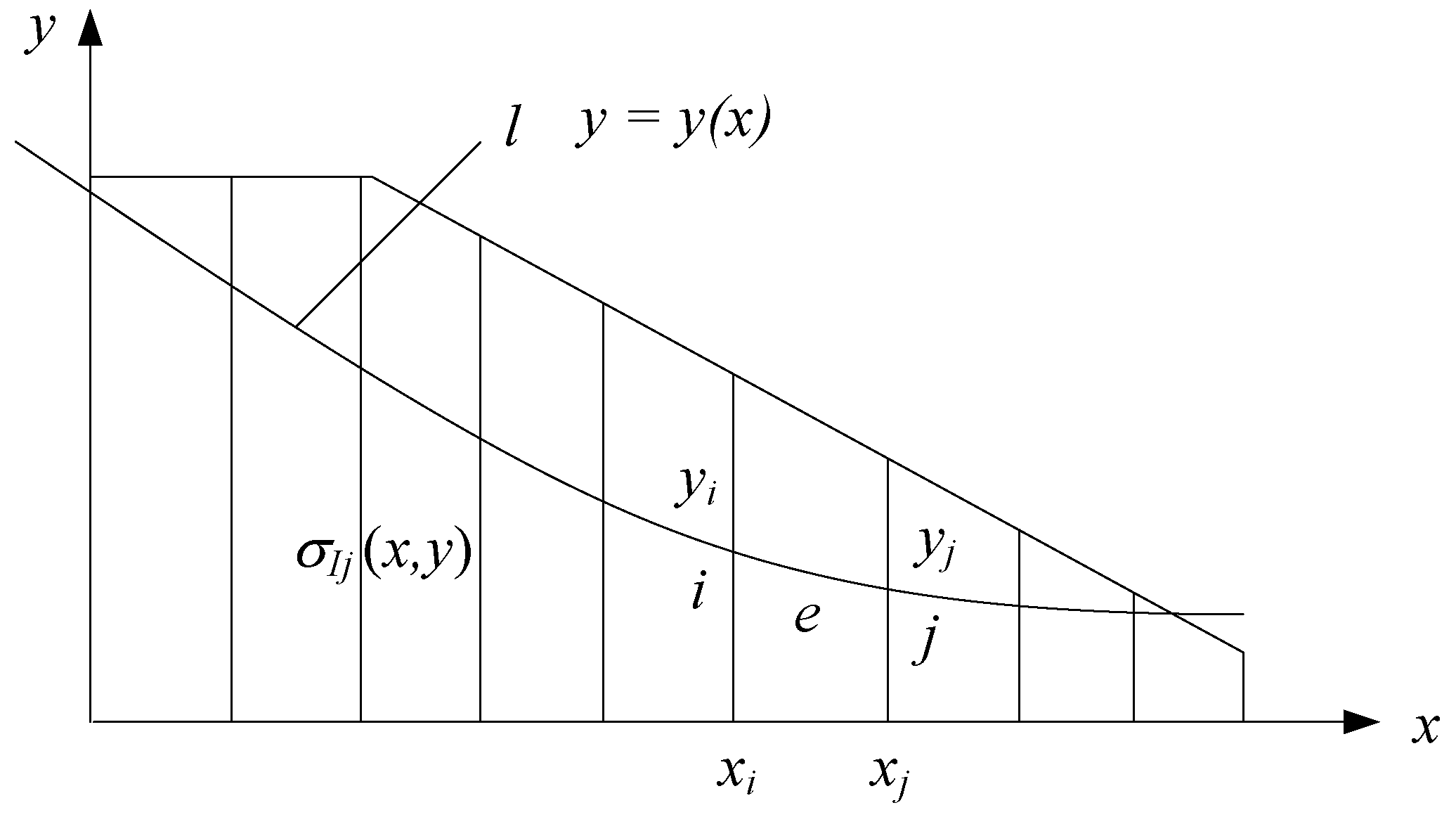
2.1. Lagrange Element Limit Analysis Principle in Soil and Rock Slopes

2.1.1. Definition of Safety Factors for Strength Reduction Methods

The slope stability analysis includes determining the most dangerous slip surface and the corresponding safety factor. For resolving the plane strain problem, the plane region of the slope studied is assumed as $S$, and the stress distribution of the rock and soil slopes in it is known. The Coulomb formula is used to calculate the shear strength $f$ of the rock and soil slopes as follows:

$$f=c+\sigma \tan \phi$$

(1)

where $\sigma$ denotes the normal stress at any point on the curve, $\phi$ represents the internal friction angle, and $c$ denotes the cohesion force. Let $l$ ($y=y(x)$) be a curve in the research area $S$; the safety factor of the rock and soil slope above $l$ along the curve is defined as follows:

$$F=\frac{{\displaystyle {\int }_0^l(c+\sigma \tan \phi )dl}}{{\displaystyle {\int }_0^l\tau dl}}$$

(2)

where $\tau$ denotes the tangential stress along curve $l$.

After dividing both sides of the above equation by $F$, we obtain

$$1=\frac{{\displaystyle {\int }_0^l(\frac{c}{F}+\sigma \frac{\tan \phi }{F})dl}}{{\displaystyle {\int }_0^l\tau dl}}=\frac{{\displaystyle {\int }_0^l(c^{\prime }+\sigma \tan {\phi }^{\prime })dl}}{{\displaystyle {\int }_0^l\tau dl}}$$

(3)

where

$$c^{\prime }=\frac{c}{F} \mathrm{and} \tan {\phi }^{\prime }=\frac{\tan \phi }{F}.$$

(4)

The left side of Equation (3) is 1, indicating that the slope reaches the ultimate equilibrium state when $c$ and $\tan \phi$ are divided by $F$.

In the safety factor calculation process, only the sliding resistance of the slope is reduced while the sliding force remains unchanged. Scholars have widely used the abovementioned method, which takes the reserve of strength parameters ($c$ and $\tan \phi$) as the definition of a safety factor. External factors acting on the slope body can cause many landslide disasters, thereby reducing strength. For example, during underground mining of end-slope coal, the strata movement and cracks caused by mining will affect the physical and mechanical parameters of the slope. Thus, the strength reduction method suits the actual situation at the site. However, the rock and soil slopes include two strength parameters ($c$ and $\tan \phi$), and the strength reduction method only provides one safety factor so the reduction in $c$ and $\tan \phi$ should be performed in the same proportion.

As shown in Figure 1, a certain number of coordinate nodes $(x_i, y_i)$ and curve elements will make $l$ discrete. The coordinate interpolation function can be constructed in the discrete curve elements, and curve $l$ can be determined through nodes $(x_i, y_i)$$(i=1, 2, \cdot \cdot \cdot \mathrm{m})$. If the value $x_i$ of the coordinate node $(x_i, y_i)$ is determined in advance, then the change in $y_i$ of curve $l$ can be obtained. The analysis of this problem can be summarized as follows. Within a given research area, the abscissas of a series of coordinate points are known, and the ordinates of these points can be changed to minimize the slope safety factor $F$ corresponding to the curve connecting them. The coordinate interpolation function can then be applied to the curve elements. First, the element of each integral point in the grid is determined and then, the stress is calculated via interpolation. Second, the Gaussian integral method is introduced to calculate the safety factor, and the critical slip surface and safety factor are obtained using the Hooke–Jeeves search method [36].

Currently, no uniform method exists for determining slope stability. Theoretically, when mechanical analysis or numerical calculation is used to determine the safety factor, if all internal and external factors affecting the stability of the slope body are considered, the slope body is unstable when the safety factor is <1. The slope body is stable when the safety factor is >1. Nevertheless, in engineering practice it is impossible to consider all the influencing factors and involve them in calculations. Thus, considering the importance of the degree of slope engineering, the integrity of geological data, and the selection of calculation parameters are crucial when selecting a safety factor. In engineering practice, according to the technical specification for annual evaluation of the stability of open-pit coal mine slopes, the value range of $F_s$ is generally 1.10–1.50 and for important projects, the range of 1.30–1.50 is advisable. For permanent works, the range of 1.15–1.25 is advisable; for temporary projects with relatively complete geological data, the range of 1.05–1.15 is advisable.

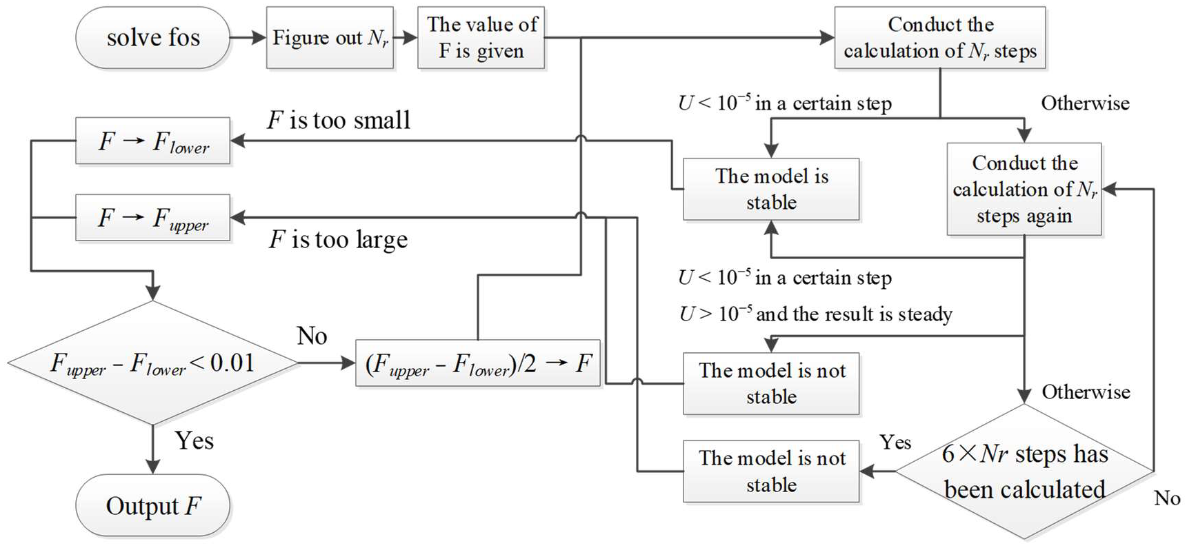
2.1.2. Basic Algorithm for Strength Reduction in the Lagrange Element

The safety factor calculated automatically using the program Flac^3D is the strength reserve safety factor. When finding the safety factor using the command solve fos (factor of safety), the program can only use this command on the Mohr–Coulomb constitutive model. Under the default setting, the program reduces the cohesion ($c$) of the material and the tangent of the friction angle ($\tan \phi$). Additionally, the user can specify the value of the tensile strength ${\sigma }_t$ and the tangent of the dilation angle to be reduced.

The idea of solving safety factors is shown in Figure 2. When the command solve fos is executed, the program first determines a “representative number of steps”, denoted as N_r, which represents the approximate number of steps required for this model to achieve equilibrium. Then, the strength parameters of the model are reduced using the given safety factor F, and the calculation of N_r steps is performed. If the maximum unbalanced force ratio U is <10⁻ⁱ, the model is considered stable, indicating that the given F value is insignificant. If U is >10⁻⁵, then the second round of calculation for obtaining N_r steps will be performed. At this point, three situations may occur. (1) When 10^−s exceeds U at a certain step, the model reaches equilibrium, indicating that the given F is insignificant. (2) In the operation process, U is maintained around a value exceeding 10⁻ⁱ for a long time and the calculation does not converge, indicating that the given F value is too large. (3) The calculation of this round of N_r steps is finished and the abovementioned two situations do not occur. For situation (3), the program will perform another round of calculations for N_r steps. If situation (3) occurs five times in a row for a given F value, it means that the model has not reached equilibrium after a total of 6 × N_r steps, indicating that the given F value is too large. If the smaller F value is taken as the lower bound F_lower and the larger F value as the upper bound F_upper, the dichotomy is used to continuously reduce the difference between F_lower and F_upper. When F_lower − F_upper < 0.01, the program terminates the calculation and outputs the current reduction coefficient F and the command solve fos is completed.

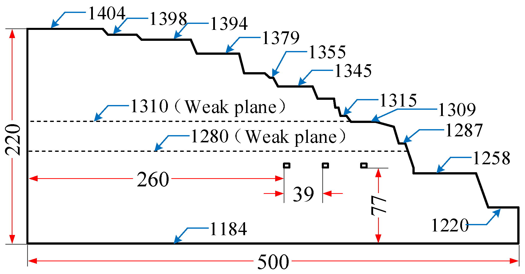
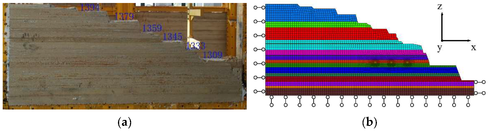
2.2. Strength Reduction Numerical Model for Stability Analysis of Disturbed Slope

Using a typical engineering geological section slope as a prototype, a numerical analysis model can be established following the geological survey report. The rock stratum of the numerical model from top to bottom and the mechanical parameters of each rock stratum are shown in

Table 1. Physical and mechanical parameters of coal and rock.

Lithology	Thickness (m)	Poisson Ratio μ	Young’s Modulus E (GPa)	Tensile Strength σt (Mpa)	Cohesion c (Mpa)	Internal Friction Angle f (°)	Density ρ (kg/m3)
Yellow earth	42	0.42	0.015	0.0125	0.125	18	1960
Weathered sandstone	14	0.36	2.0	0.2500	2.500	38	2300
Sandstone 1	30	0.32	4.2	0.3000	3.000	39	2380
Mudstone	24	0.34	2.8	0.2000	2.000	38	2490
Silty sandstone 1	12	0.32	4.6	0.3500	3.500	36	2320
Sandstone 2	12	0.30	5.5	0.4000	4.000	40	2380
4# Coal seam	8	0.38	1.0	0.2950	1.620	36	1440
Shale 1	10	0.33	2.4	0.3000	3.000	42	2450
Silty sandstone 2	14	0.32	4.8	0.5000	5.000	38	2600
Shale 2	8	0.35	3.0	0.5000	5.000	38	2580
9# Coal seam	13	0.36	1.2	0.2950	1.620	39	1330
Sandstone 3	10	0.28	6.9	0.5000	5.000	41	2380
11# Coal seam	5	0.35	1.3	0.2950	1.620	36	1400
Sandstone 4	18	0.25	12.0	0.5000	5.000	44	2600

. The bottom elevation of the model is 1184 m, and the elevation of the lowest step is 1220 m; there is rock stratum between them. The top elevation is 1404 m. The model has a total of 11,142 nodes and 5421 units. The length of the model in the x direction is 500 m, its height in the z direction is 220 m, and its thickness in the y direction is 1.5 m. In the y direction, only one layer of units is divided. The two sides and the bottom of the model are the roller boundary conditions, and the degree of freedom of all nodes in the y direction is constrained to simulate the plane strain problem. Figure 3 shows the model size and elevation of its main parts. Figure 4 shows the grid, grouping, and boundary conditions of the numerical model. The simulated excavation is approximated by the following steps. The gob units are first given small deformation and strength parameters, and the Poisson’s ratio is set approximate to 0, then the stress state of the gob units is cleared.

2.3. Slope Deformation and Critical Slip Surface Evolution Law during Underground Mining in the End Slope

2.3.1. Characteristics of the Displacement of the Disturbed Slope

In the physical simulation test, the proportions of river sand, calcium carbonate, gypsum, and water were determined and their weighting was performed according to rock properties. The mixed materials were spread along the horizon direction, and a tamp hammer was used to compact the materials; mica powder was scattered on the outline of the slope, which made the excavation more accurate. Due to the influence of underground excavation, the maximum deformation rates of steps reached 2.6 mm/h in engineering practice monitoring. Considering the size limitation of the test platform, the model size includes a length of 2.50 m, a height of 1.06 m, and a width of 0.20, and the geometry similarity ratio is $C_l$ = $l_p/l_m$ = 150:1. The characteristics of the displacement of the disturbed slope are shown in Figure 5.

(1)

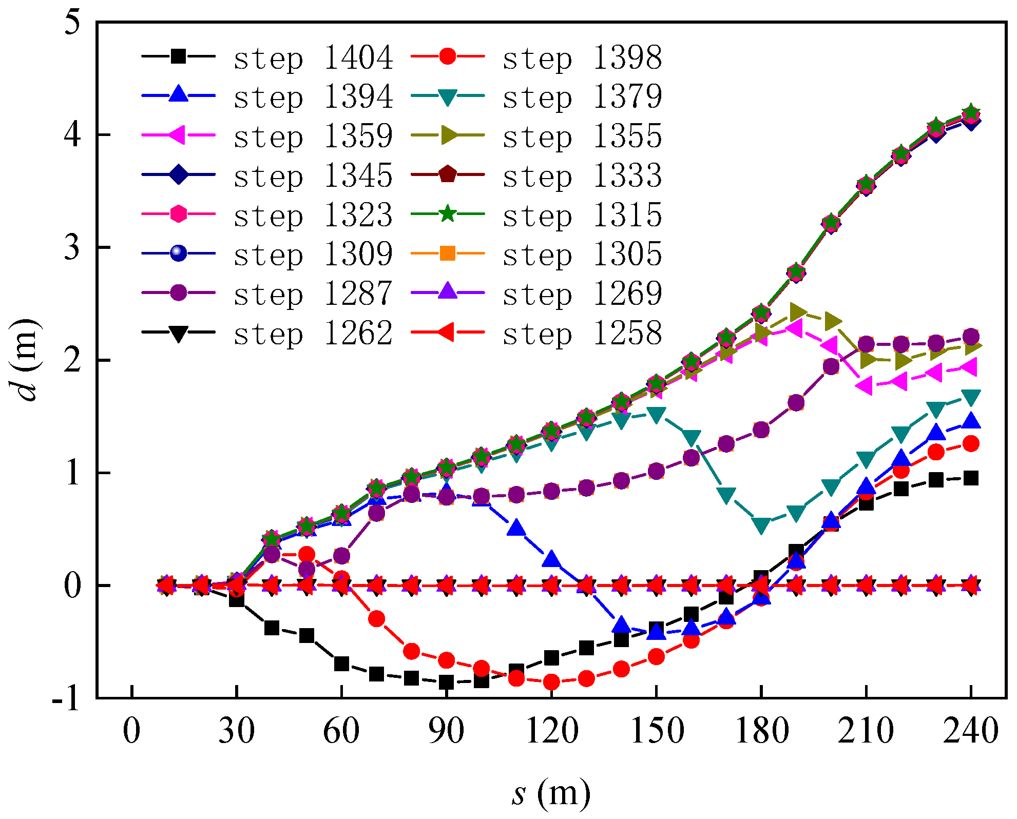
Horizontal displacement of steps

The advancing working face of the underground mine breaks the original stress equilibrium state of the underground rock mass; the rock strata deform, the slope is disturbed violently, and the steps move considerably horizontally. Figure 6 shows the changing curve of the horizontal displacement d of each step top with the advancing distance s of the working face. Figure 7 shows the horizontal displacement nephogram of the disturbed slope as the working face advances.

Table 2. Horizontal displacement of steps (m).

Advancing Distance (m)	30	60	90	120	150	180	210	240
Step 1404	−0.123	−0.693	−0.860	−0.642	−0.386	0.071	0.733	0.955
Step 1398	−0.029	0.059	−0.664	−0.857	−0.631	−0.110	0.829	1.260
Step 1394	0.013	0.583	0.820	0.219	−0.429	−0.115	0.866	1.445
Step 1379	0.031	0.618	1.006	1.286	1.530	0.548	1.135	1.684
Step 1359	0.032	0.628	1.035	1.360	1.741	2.210	1.773	1.940
Step 1355	0.032	0.629	1.036	1.361	1.750	2.246	2.007	2.129
Step 1345	0.029	0.634	1.041	1.369	1.788	2.410	3.542	4.022
Step 1333	0.027	0.635	1.042	1.371	1.789	2.411	3.547	4.064
Step 1323	0.026	0.637	1.044	1.372	1.792	2.416	3.555	4.078
Step 1315	0.024	0.642	1.047	1.375	1.796	2.424	3.567	4.099
Step 1309	0.022	0.262	0.783	0.835	1.013	1.380	2.140	2.006
Step 1305	0.022	0.263	0.783	0.836	1.013	1.380	2.140	2.007
Step 1287	0.022	0.264	0.786	0.838	1.016	1.382	2.142	2.009
Step 1269	0.002	0.000	−0.002	−0.002	0.000	0.001	0.001	0.002
Step 1262	0.002	0.000	−0.001	−0.001	0.001	0.001	0.002	0.002
Step 1258	0.001	0.000	0.000	0.000	0.001	0.001	0.001	0.001
Step 1220	0.000	0.000	0.000	0.000	0.000	0.000	0.000	0.000

presents the horizontal displacement values of the steps. According to the forms of the d–s curves of different steps, these steps can be divided into different parts.

i.

The step on the upper slope is affected by mining subsidence and slope deformation. Its d–s curve generally presents an upward–downward–upward pattern, and the decline range is obvious. Slope deformation mainly affects the horizontal displacement of the step during the ascending stage of the curve. However, in the descending stage of the curve, mining subsidence primarily affects the horizontal displacement of the step. The value of s corresponding to the inflection point of the curve from rising to falling is the corresponding advancing distance of the working face when the influence of mining subsidence on the horizontal displacement of the step is enhanced. Taking Step 1398 as an example, in the process of advancing the working face from 0 to 50 m, the top of the slope is located outside the goaf boundary (on the right side of the boundary) and mining subsidence insignificantly affects its movement. However, due to the mining disturbance, the slope body deforms and drives the step toward the mined-out area (move toward the right), which is shown by the increase in its horizontal displacement and the rise in the d–s curve. The step is located within the boundary when the working face advances from 50 to 120 m. Affected by the collapse of the overlying strata of the goaf, the step moves away from the free face, showing that its horizontal displacement decreases and the d–s curve decreases. When the working face continues to advance beyond 120 m, as the step is located directly above the goaf, the mining subsidence mainly causes the step to move downward. Slope deformation again becomes the main factor inducing the horizontal movement of the step. The step moves toward the goaf again, and the d–s curve rises.

ii.

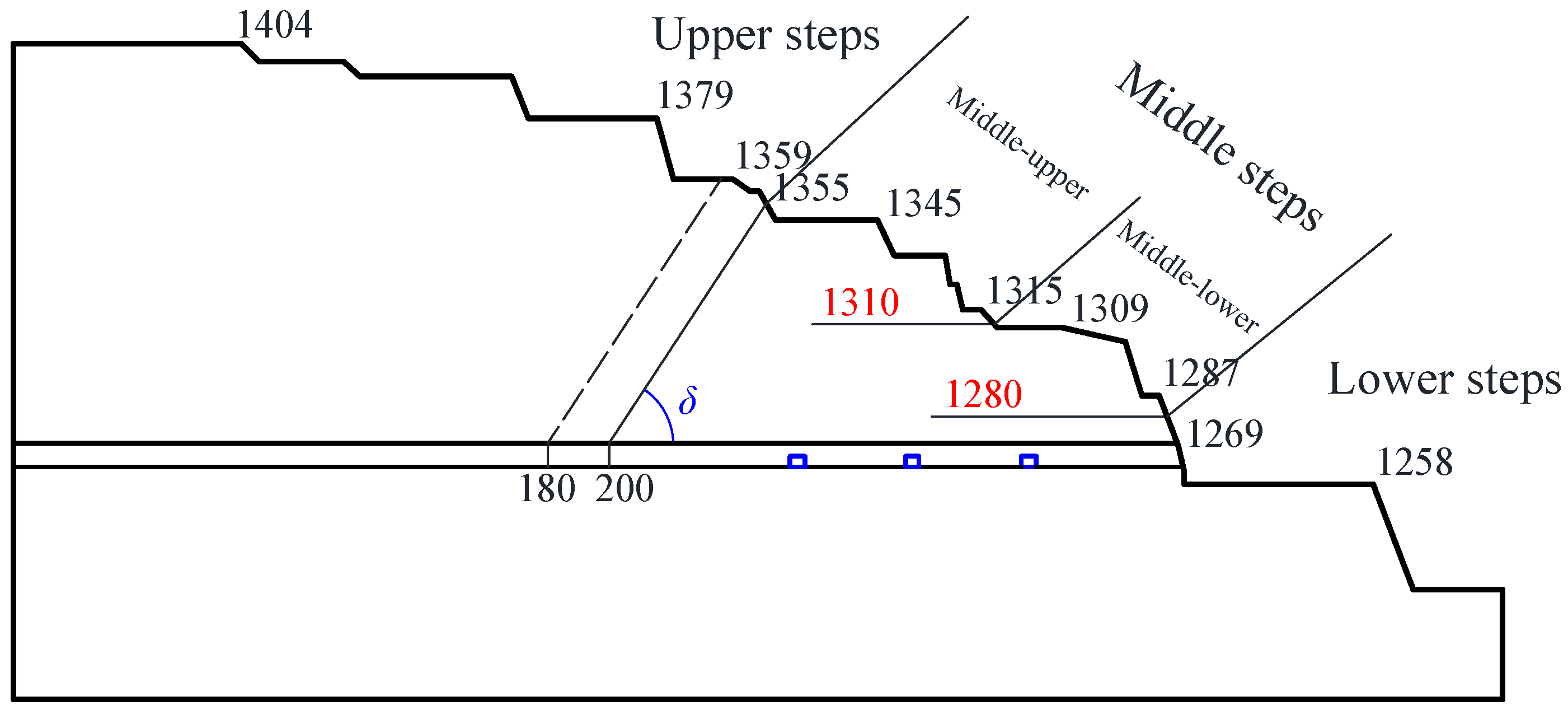
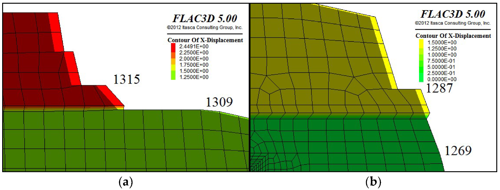
The step in the middle of the slope is always outside the boundary line when the working face advances to the stop mining line. The influence of slope deformation on the horizontal movement of the step exceeds that of mining subsidence, and the d–s curve generally presents a rising trend with no obvious decline interval. These steps can be divided into two parts via the 1310 weak plane. The steps above the 1310 weak plane are affected simultaneously by the slip of the two weak planes and their horizontal displacements are large. Steps from 1309 to 1287 are located between two weak planes; therefore, they are only affected by the slip of weak plane 1280, and the horizontal displacement is small.

iii.

The mining subsidence and slope deformation slightly affect the steps below the 1280 weak plane. The d–s curve is almost a horizontal line; hence, the horizontal displacement value is 0 m.

When the working face advances to 180 m, the parts of the steps from Step 1359 to 1404 denote the upper steps, Steps 1287 to 1359 represent the middle steps, and Steps 1258 to 1269 denote the lower steps. The maximum horizontal displacement occurs at Step 1315, which is 2.42 m. When the working face continues to advance to 200 m, Steps 1355 and 1359 are within the boundary and become the upper steps (Figure 8). Figure 6 shows that ① the horizontal displacement curves of steps in all parts are similar, indicating that the local-slip phenomenon with steps as the unit is not obvious, and the disturbed slope slip is manifested as the overall slip of the upper, middle-upper, middle-lower, and lower parts; ② as the working face advances, when a step gradually evolves from the middle-upper step to the upper step, its curve will deviate from the trajectory of other middle-upper steps and then presents a typical curve shape of upper steps; ③ when advancing from 190 to 240 m, the horizontal displacement of the middle step increases. The maximum horizontal displacement increases from 2.79 to 4.2 m, and the slope slips violently.

(2)

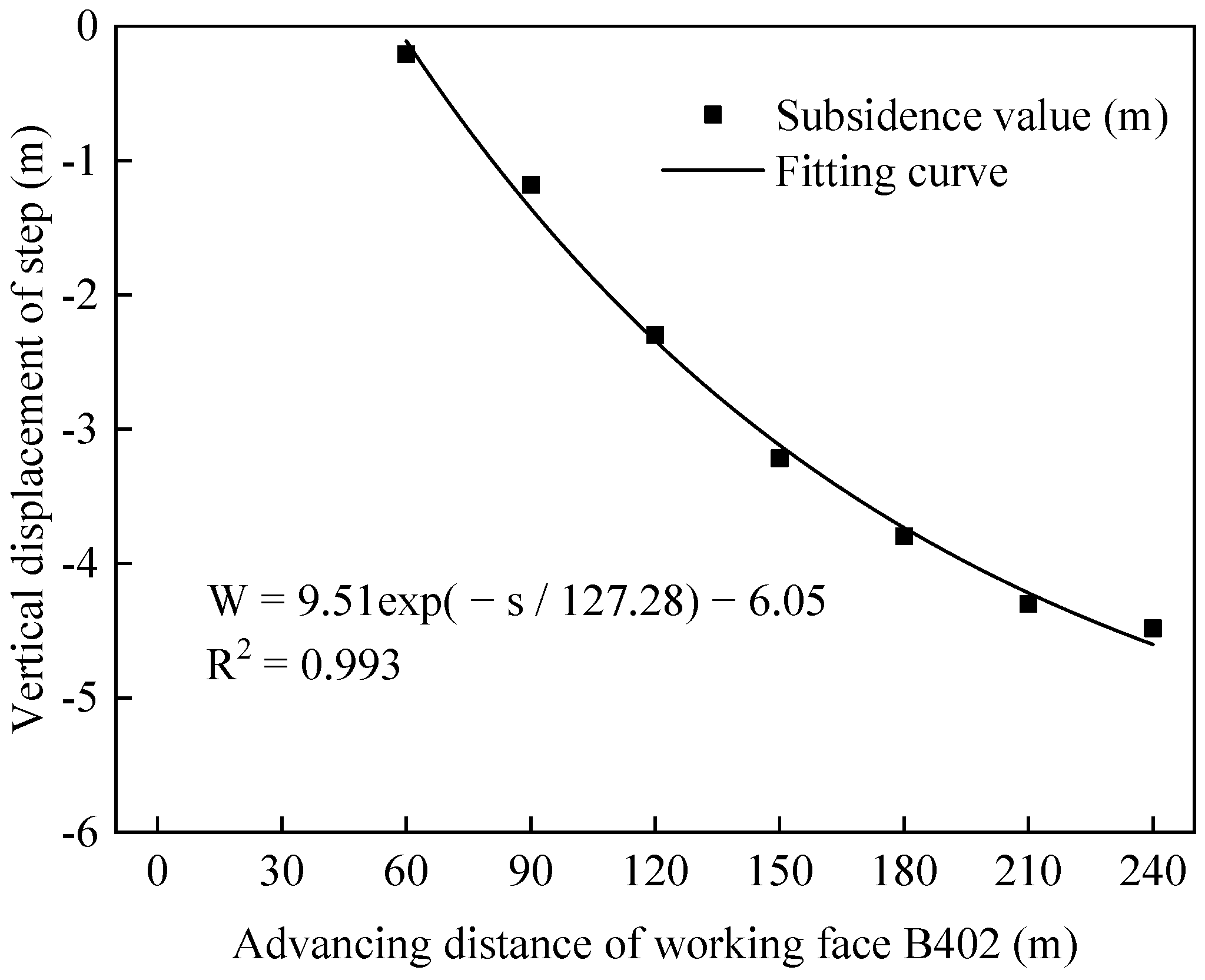
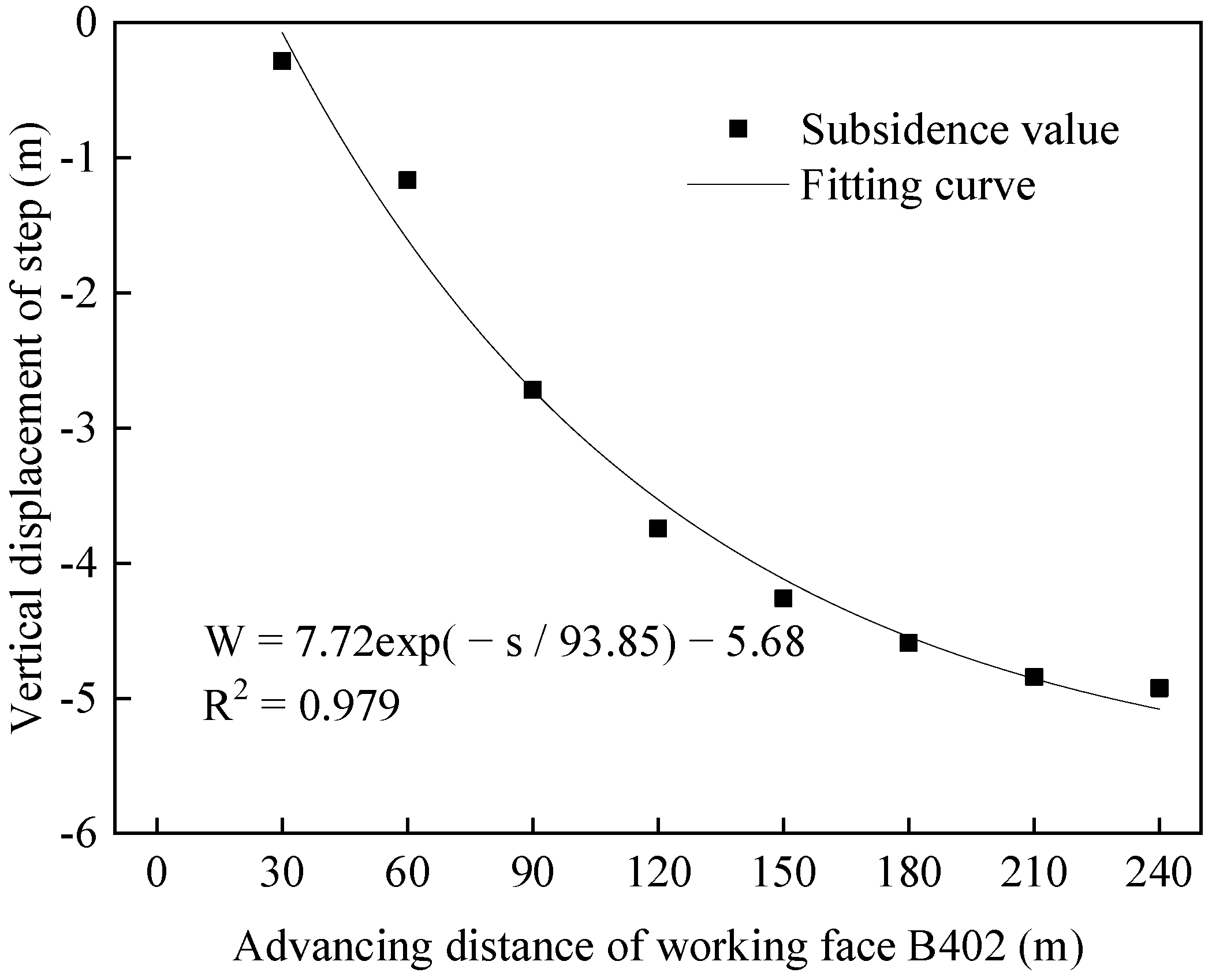
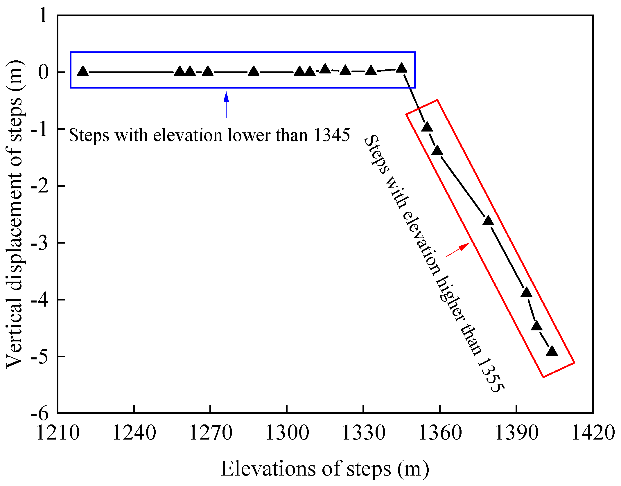
Vertical displacement of steps

Table 3. Vertical displacement of steps during working face advancement.

Advancing Distance (m)	30	60	90	120	150	180	210	240
Step 1404	−0.282	−1.165	−2.716	−3.743	−4.260	−4.590	−4.842	−4.925
Step 1398	−0.029	−0.207	−1.182	−2.299	−3.217	−3.796	−4.300	−4.482
Step 1394	−0.005	−0.013	−0.072	−0.501	−1.149	−2.162	−3.301	−3.891
Step 1379	−0.002	−0.004	−0.007	−0.023	−0.059	−0.355	−1.576	−2.630
Step 1359	−0.002	−0.004	−0.005	−0.008	−0.015	−0.042	−0.423	−1.396
Step 1355	−0.002	−0.003	−0.004	−0.006	−0.005	−0.008	−0.063	−0.982
Step 1345	−0.002	−0.002	−0.003	−0.002	−0.002	−0.004	−0.008	0.057
Step 1333	−0.001	0.001	0.000	0.001	0.002	0.004	0.006	0.012
Step 1323	−0.001	0.002	0.001	0.002	0.004	0.006	0.009	0.017
Step 1315	0.000	0.005	0.003	0.008	0.013	0.020	0.028	0.043
Step 1309	−0.001	−0.001	−0.001	−0.001	−0.001	−0.001	−0.002	−0.002
Step 1305	0.000	0.001	0.002	0.001	0.001	0.001	0.000	0.000
Step 1287	0.001	0.002	0.003	0.002	0.002	0.001	0.001	0.001
Step 1269	0.000	0.001	0.002	0.002	0.001	0.001	0.001	0.000
Step 1262	0.000	0.001	0.002	0.002	0.001	0.001	0.000	0.000
Step 1258	0.000	0.000	0.000	0.000	0.000	0.000	0.000	0.000
Step 1220	0.000	0.000	0.000	0.000	0.000	0.000	0.000	0.000

presents the vertical displacement values of all the steps in the working face advancement project. Steps 1355–1404 exhibit subsidence deformation owing to mining disturbances. With an increase in the mining distance, the subsidence value of the step increases gradually. When the steps (Steps 1398 and 1404) are completely affected by mining, their subsidence value first increases rapidly and then slowly. The following exponential fitting formula can be used to present the variation law of the step-subsidence value for advancing working faces:

$$W=A\times e^{(\frac{-s}{b})}+y_0$$

(5)

where $W$ denotes the step-subsidence value (unit: m) and $s$ represents the advancing distance of the working face (unit: m). Figure 9 and Figure 10 show the vertical displacements of Steps 1398 and 1404 during the advancing process of the working face, respectively. The fitting formulas for vertical displacements are shown in Equations (6) and (7), and the fitting coefficients are 0.993 and 0.979, respectively.

$$W=9.51\times e^{(\frac{-s}{127.28})}-6.05 \mathrm{and}$$

(6)

$$W=7.72\times e^{(\frac{-s}{93.85})}-5.68$$

(7)

When the working face advances to 240 m, the subsidence values of all the steps reach their maximum. With a decrease in step elevation, the maximum subsidence value of the steps gradually decreases. The subsidence deformation value of the steps with an elevation ≤1345 is very small and they are almost unaffected by the subsidence of mining (Figure 11).

With an increase in the advancing distance, the subsidence caused by mining gradually develops downward from Step 1404, and the subsidence values of the steps disturbed via mining gradually increase.

(3)

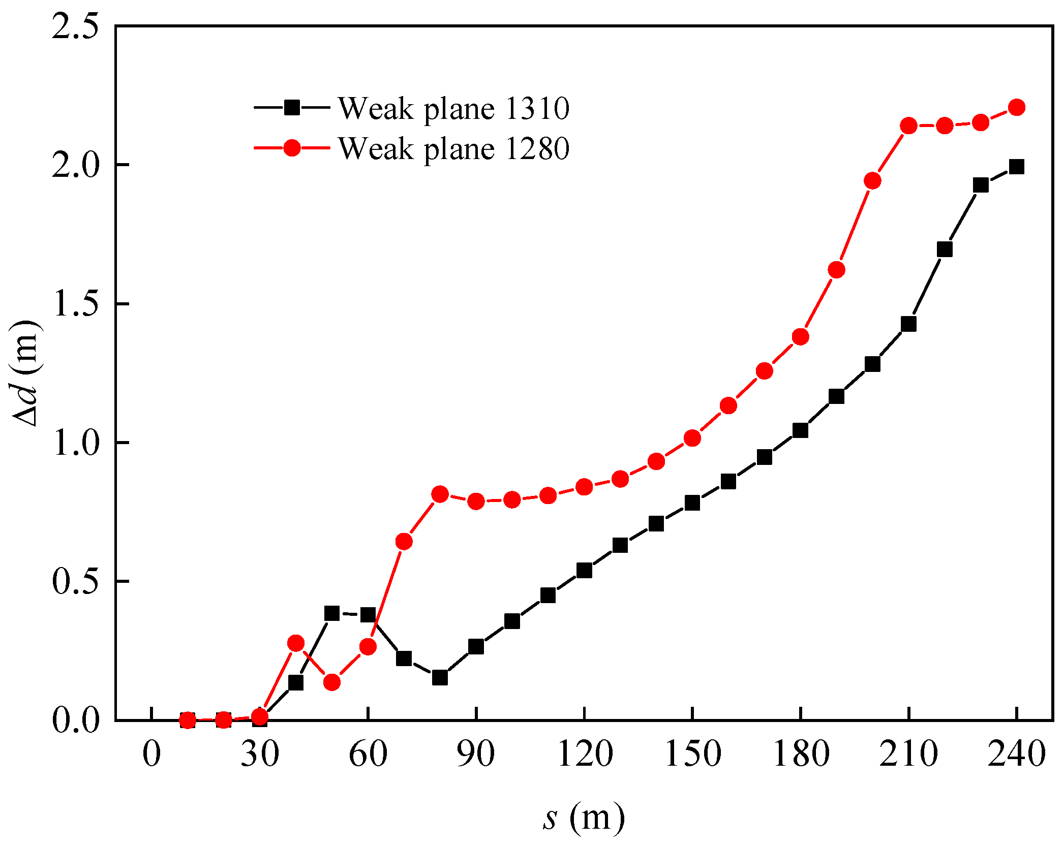
Slipping of weak interlayer

The weak interlayer refers to a layer that is thinner than the adjacent strata and with clearly smaller physical and mechanical parameters. When the weak interlayer is argillated by the action of atmospheric precipitation or groundwater, it is called an argillated interlayer or argillated weak interlayer. The formation of weak interlayers is closely related to geologically diagenetic conditions and tectonic processes, and they can be divided into primary, secondary, and structural weak interlayers according to their origins. Primary weak interlayers refer to intercalation with low strength and deformation parameters and poor cementation between hard strata during the formation of rock masses, such as tuffaceous shales, thin layers of clay rocks, and chlorite enrichment zones in metamorphic rocks. A secondary weak interlayer is formed through argillization, or the debris formation of mineral-filled joints and primary weak interlayers under the action of water and weathering. Most of these layers are distributed at shallow depths, and the physical and mechanical properties of rock and soil mass, hydrogeological conditions, and landforms affect them considerably. The secondary weak interlayer is partially argillated or softened, and the content of water and clay particles is high. A structural weak interlayer is formed via rock mass fracture and granulation due to the dislocation of soft rock or rock strata contact surfaces under the action of tectonic forces. The cohesion and internal friction angle of a weak interlayer are 40.52 kPa and 30°, respectively.

The deformation of a rock mass comprises rock deformation and the deformation of a structural plane. The stress–strain curve is similar to that of rock. Nevertheless, owing to the existence of a weak structural plane, the deformation value of the rock mass under the same stress level exceeds that of the rock. A hyperbolic or exponential function can be used to describe the effect of normal stress on the structural plane and crack, which is a nonlinear process.

Based on a large number of experimental data, Goodman, et al. provided the following empirical formula for the closure deformation of a structural plane:

$$\sigma =\frac{\Delta b}{b_0-\Delta b}{\sigma }_i+{\sigma }_i$$

(8)

where $\sigma$ denotes normal stress, $\Delta b$ represents the closing volume of the structural plane, $b_0$ denotes the maximum closure error, and ${\sigma }_i$ represents the emplacement stress.

Bandis, et al. conducted deformation tests on the structural planes with different weathering degrees and lithology and provided the normal deformation equation of cracks and the directional stiffness expression of the structural plane:

$$\sigma =\frac{\Delta b}{m-n\Delta b}$$

(9)

$$K_n=\frac{\partial \sigma }{\partial \Delta b}=\frac{1}{m{(1-\frac{n}{m}\Delta b)}^2}=\frac{K_{ni}}{{(1-\frac{\Delta b}{b_0})}^2}$$

(10)

where $m$ and $n$ are constants; $\sigma \to \infty$, $\frac{m}{n}\to \Delta b=b_0$; $\sigma \to 0$, $m=\frac{1}{K_{ni}}$; $K_{ni}$ denotes the initial directional stiffness of the structural plane.

When the normal stress is constant, the lateral load is applied to the rock mass in the structural plane and the relation curve between shear stress τ and shear displacement ν can be obtained. The peak strength and residual strength can be observed in the shear deformation curves of rigid structural planes, except for the intercalated clay layers, the broken interlayers, and the joint planes with thick fillings. When the shear displacement is small, it is characterized by elastic deformation, and the shear stress increases linearly with increasing shear displacement. When the shear displacement continues to increase, the slope of the curve decreases until the shear stress reaches its peak strength. Afterward, the shear stress decreases and becomes stable as the shear displacement increases.

A certain roughness exists on the fracture surface of the rock mass in the site, which presents a dilatancy property under a shear action. The dilatancy property will increase the width of the fracture and induce a change in the seepage channel.

The relation between shear deformation and shear stress of a fracture is as follows:

$$d\tau =K_{s}dv$$

(11)

where $K_s$ denotes the shear stiffness of the fracture surface.

When the dilatancy effect occurs on the fracture surface, the following relation is satisfied:

$$du=dv\tan i$$

(12)

where $u$ denotes normal deformation, $v$ represents shear deformation, and $i$ denotes the dilatancy angle.

Substituting Equation (11) into Equation (12), we can obtain

$$du=\frac{d\tau }{K_s}\tan i$$

(13)

Integrating Equation (13), we can obtain

$$u={\displaystyle \underset{\tau 1}{\overset{\tau 2}{\int }}\frac{\tan i}{K_s}}d\tau$$

(14)

On the rock slope, the stress concentration easily forms near the weak interlayer. When the stress value exceeds the strength of the weak interlayer, local failure occurs and the failure gradually develops to form a slip surface.

In the numerical simulation, the structural plane can be simulated in two ways: a weak interlayer or a contact element without thickness. This study uses the first method. A solid plane element was used to simulate the weak rock strata and rock mass. Nevertheless, the structural plane uses lower strength and deformation parameters than matrix rock. In the calculation process, the strength parameters of the rock mass and structural plane are reduced simultaneously until the slope reaches the ultimate equilibrium state, where the safety factor of the slope body can be obtained.

The difference between the horizontal displacements of Steps 1309 and 1315 and Steps 1269 and 1287 are taken as the relative slip distances (hereinafter referred to as weak-plane slipping) of the upper and lower strata on weak planes 1310 and 1280, respectively. Figure 12 shows the simulation result of a weak-plane slipping at an advancing distance of 180 m, in which the dark area represents the original position of the slope. Figure 13 shows the variation law of the slipping distance Δd of a weak plane with the advancing distance s of the working face. Figure 13 shows that (1) the two Δd–s curves of weak planes show a general upward trend. The slipping distances of the weak planes 1310 and 1280 increase considerably at the advancing distances of 220 and 190 m. (2) Generally, the slipping distance of the weak plane 1280 exceeds that of the weak plane 1310. This is because the relative position of weak plane 1280 is lower and it bears a greater load than weak plane 1310. Due to the influence of weak-plane slipping, the maximum deformation rate of steps reached 2.6 mm/h in engineering practice monitoring.

2.3.2. Position and Shape Evolution of the Critical Slip Surface

Two nephograms can represent the critical sliding surfaces. (1) Flac^3D calculates the slope safety factor based on the model convergence criterion. When the calculation does not converge, the plastic flow will continue to occur along a certain path for the slipping mass; accordingly, the plastic shear strain will continue to occur for all elements along the path. To exclude some elements in other areas that have undergone large plastic shear strain but are now in a stable state, the position of the path, i.e., the position of the critical slip surface, can be presented using the nephogram of the plastic shear strain rate. (2) The displacement of the slipping mass increases as it slides along the critical slip surface. By contrast, other regions remain relatively stable, allowing the displacement nephogram to indicate the slip mass position.

Notably, the “displacement” mentioned here refers to the displacement of the model after strength reduction in a specific calculation step and is not the real displacement of the model. Taking the initial slope of an unexcavated roadway as an example, the initial slope is in a stable state and all displacement values should be 0. When solving the safety factor, the original model will eventually be reduced to a critical state and the slide body will have plastic flow. When the program exits the calculation, the displacement value of the slipping mass will not be 0. This displacement is not a real displacement, has no practical significance, and can only be used to indicate the range of the slipping mass. Thus, the displacement in this section should be distinguished from the displacement in other sections.

Figure 14 shows the forms of the critical sliding surfaces of the disturbed slope and the corresponding safety factors when the working face advances to different positions. The subfigures presented on the left side show the plastic shear strain rate nephograms, and those on the right side show the displacement nephograms. Figure 15 shows the variation curve of the slope safety factor F with the advancing distance s. Figure 14 and Figure 15 indicate the following:

(1)

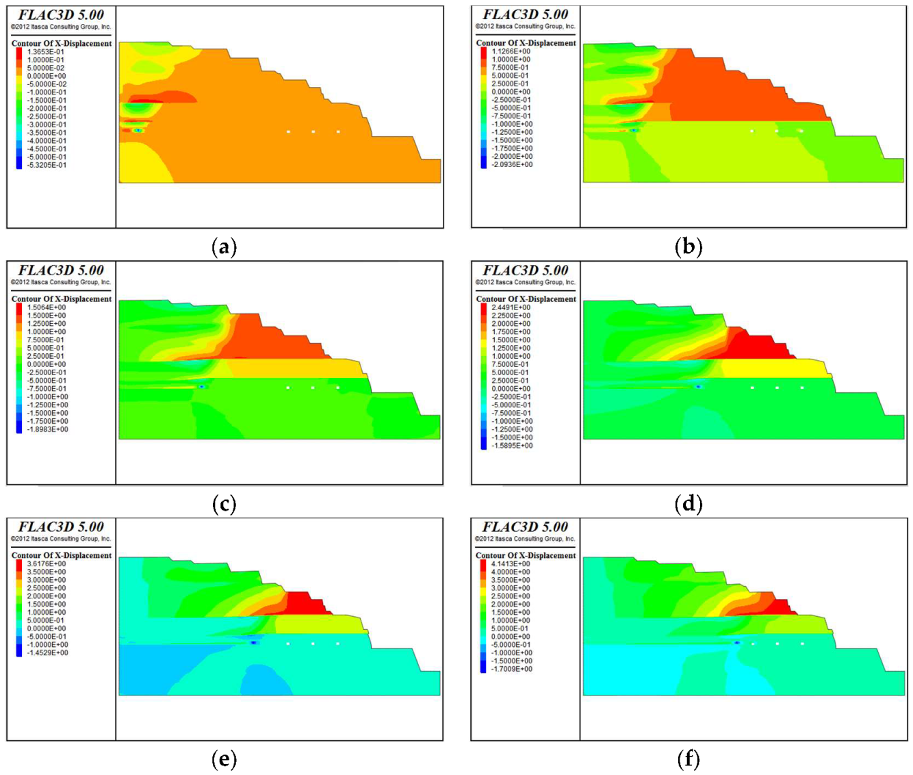
The initial slope mainly contains three critical sliding surfaces. The main sliding surface is from Step 1404 to the weak surface 1280, and the main slip mass cuts along the weak surface 1280 and the slope surface of Step 1287. The secondary sliding surface is from the flat plate 1404 to the 9# coal seam, and the secondary slip mass cuts along the 9# coal seam at the slope foot of Step 1258. A local critical sliding surface is observed in Step 1379, which mostly comprises loess with low strength, is the step with the steepest slope in the loess soil layer, and has the tendency to landslide.

(2)

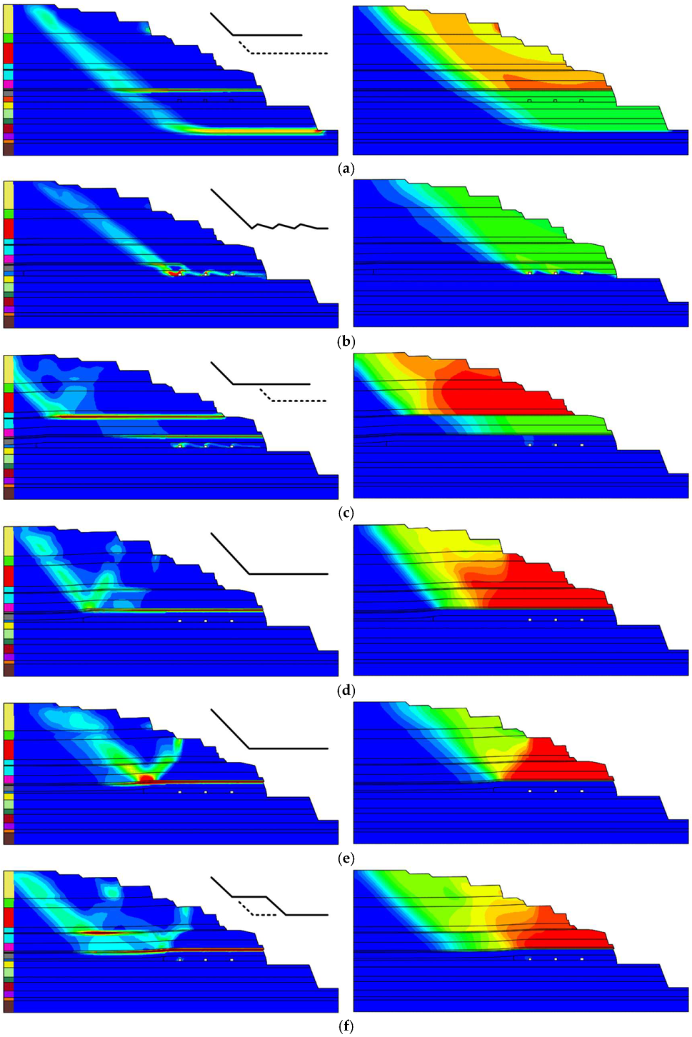
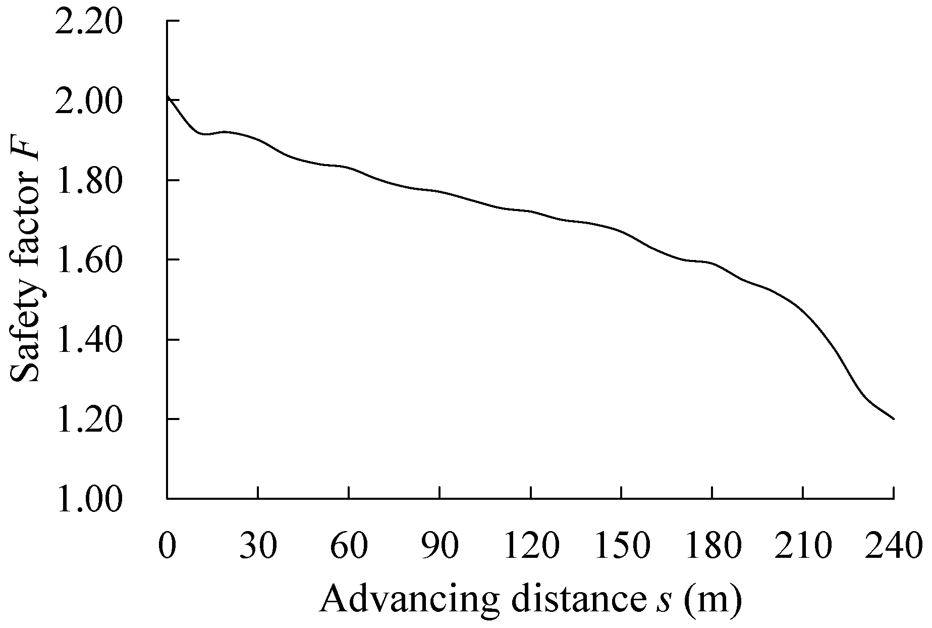
After roadway excavation, when the advancing distance of the working face is between 0 and 30 m, the position and form of the critical sliding surface remain unchanged (Figure 14b). The critical sliding surface extends from Step 1404 to the left side of the auxiliary roadway of the 4# coal seam. The three roadways are taken as the base point and extend in a zigzag shape to the slope foot of Step 1262. The slip mass cuts from the slope foot of Step 1262. In this interval, the safety factor does not change and the mining disturbance slightly influences slope stability.

(3)

When the advancing distance of the working face is between 40 and 50 m, the position and shape of the critical sliding surface remain unchanged (Figure 14c). The main sliding surface extends from Step 1404 to the weak plane 1310, and the main sliding body is cut out along the weak plane 1310 at the slope foot of Step 1315. The secondary sliding surface extends from the weak plane 1310 to the weak plane 1280, and the secondary slip mass cuts along the weak plane 1280 and the slope surface of Step 1287. The nephogram of the plastic shear strain rate shows that the roadway of the 4# coal seam is also seriously sheared, but the shearing surface does not develop upward or form a sliding plane. In this interval, the safety factor clearly decreases.

(4)

When the advancing distance of the working face is between 60 and 210 m, the form of the critical sliding surface is unchanged and the position moves toward the free face with the advancing of the working face (Figure 14d,e). The critical sliding surface extends from Step 1404 or slope foot to the weak plane 1280, and the sliding body cuts from Step 1287 along the weak plane 1280. During this interval, the safety factor continues to decrease.

(5)

When the advancing distance of the working face is between 220 and 240 m, the position and form of the critical sliding surface remain unchanged (Figure 14f). The main sliding surface extends from Step 1404 to the weak plane 1310. After developing along the weak plane 1310 for a certain distance, it continues to extend downward to the weak plane 1280 in the form of a W (double L)-shaped broken line. The main slip mass cuts along the weak plane 1280 and the slope surface of Step 1287. The secondary sliding surface extends from the weak plane 1310 to weak plane 1280 and intersects with the main sliding surface. In this interval, the factor of safety decreases rapidly. Zhu, et al. [37] adopted a numerical simulation to optimize the boundary parameters and concluded that when the horizontal distance between the open-off cut and the slope was increased by 20 m, the overall stability of the slope would be significantly improved.

(6)

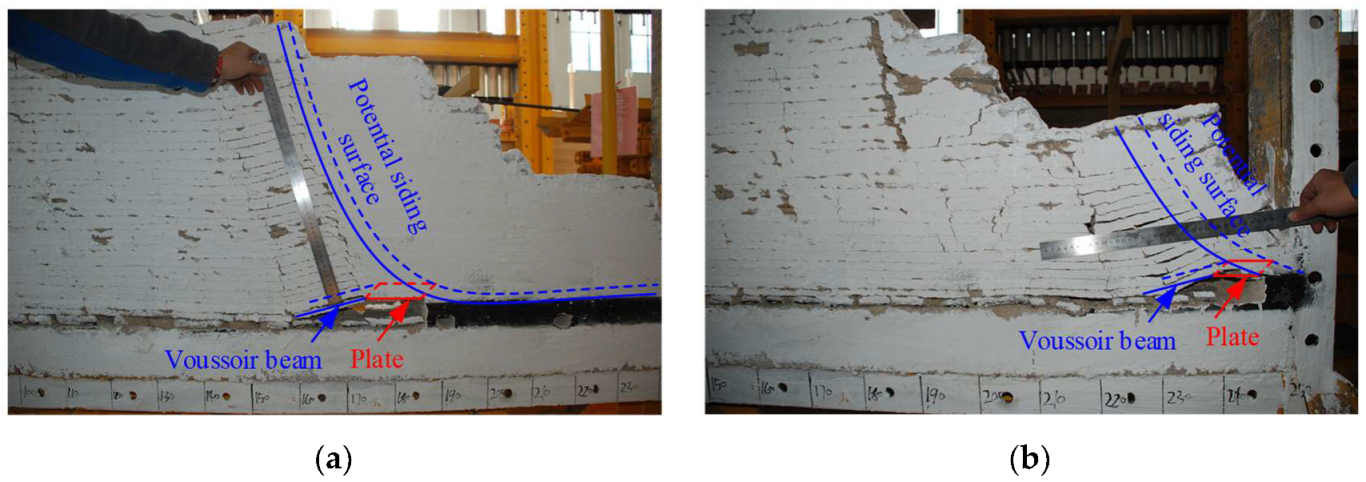
When the working face advances for more than 30 m, there is also a sliding surface (called an inner sliding surface) in the slipping mass. The position of the inner sliding surface roughly coincides with the goaf boundary (Figure 14c–f). Moreover, because of the influence of mining subsidence, the rock mass near the boundary line undergoes shear failure due to subsidence, which decreases the strength. Chang, et al. [38] studied the rock damage evolution in the coordinated open pit with underground mining area using the numerical simulation method; the results showed that the slope damage was mainly caused by the collapse of underground goaf. Nevertheless, the original sliding surface is not smooth owing to the weak surface. It presents an obvious L-shaped broken line; therefore, the sliding body itself will considerably deform while sliding and constantly accumulate strain energy. Under the combined action of these two factors, the slipping mass will eventually cut along the rock mass with lower strength and the inner slip surface will form. The sliding body on the left of the inner sliding surface slides downward under gravity, and the sliding body on the right slides horizontally toward the free face due to the push from the slipping mass on the left.

Based on the theoretical analysis and physical experiments, a “Voussoir beam–plate–slip surface” structure model is established (Figure 16), which helps understand the deformation and failure process. The shapes of potential siding surface are basically the same in the numerical simulation and physical model.

The grid density of the numerical model also affects the simulation results. When the 11# coal seam divided into two layers, the safety factors of the initial slope and the 240-meter excavation slope are 1.98 and 1.17, respectively, decreasing by 1.49% and 2.50% compared to the values when divided into one layer.

The strata behavior of underground mining on the end slope differs from traditional mining and the disturbance may lead to a landslide. This study can deepen our understanding of the overlying strata movement law and the control of underground mining at the end slope.

3. Conclusions

The slope stability and evaluation method of underground mining of end-slope coal were studied in the rock-stability analysis using the Lagrange element strength reduction method. The geological conditions for mining in the coordinated open pit with an underground mining region of the Anjialing Open-Pit Mine and Underground No. 2 Mine were used to establish a numerical analytical model. The evolution law of slope stability in open-pit end-slope mining was studied using the proposed numerical simulation method, and the following conclusions were drawn:

(1)

The steps have obvious horizontal movement and deformation under the influence of underground mining disturbances. Taking the horizontal displacement at the slope tops of the steps as the deformation index, the entire disturbed slope can be divided into four regions: upper, middle-upper, middle-lower, and lower steps.

(2)

The weak interlayer is an important factor affecting the deformation of the disturbed slope. As the working face advances, the sliding distance of the weak surface increases. When the advance distance exceeds a certain value, the sliding distance increases considerably and the sliding distance of the lower weak plane exceeds that of the upper weak plane.

(3)

When underground mining fully affects a step, its subsidence value first increases rapidly and then slowly. The exponential function $W=A\times e^{(\frac{-s}{b})}+y_0$ can represent the change rule of the step-subsidence value during working face advancing.

(4)

The development of critical sliding surfaces can be tracked through the distribution of the plastic shear strain rate and deformation. In underground mining, the critical sliding surface of the slope will develop along the soft rock or coal seam, showing the L-shaped or W (double L)-shaped broken line. As the working face advances, the initial position of the sliding mass remains unchanged while the cutting position alternately changes up and down in the weak plane. When the advancing distance exceeds a certain value, the safety factor drops sharply, providing a basis for selecting an appropriate working face stop line.

References

- Bakhtavar, E.; Shahriar, K.; Mirhassani, A. Optimization of the transition from open-pit to underground operation in combined mining using (0–1) integer programming. J. S. Afr. Inst. Min. Metall. 2012, 112, 1059–1064. [Google Scholar]
- Bakhtavar, E.; Shahriar, K.; Oraee, K. Mining method selection and optimization of transition from open pit to underground in combined mining. Arch. Min. Sci. 2009, 54, 481–493. [Google Scholar]
- Epstein, R.; Goic, M.; Weintraub, A.; Catalan, J.; Santibanez, P.; Urrutia, R.; Cancino, R.; Gaete, S.; Aguayo, A.; Caro, F. Optimizing Long-Term Production Plans in Underground and Open-Pit Copper Mines. Oper. Res. 2012, 60, 4–17. [Google Scholar] [CrossRef]
- Opoku, S.; Musingwini, C. Stochastic modelling of the open pit to underground transition interface for gold mines. Int. J. Min. Reclam. Environ. 2013, 27, 407–424. [Google Scholar] [CrossRef]
- Sokolov, I.V.; Smirnov, A.A.; Antipin, Y.G.; Baranovsky, K.V. Rational design of ore discharge bottom in transition from open pit to underground mining in udachny mine. J. Min. Sci. 2013, 49, 90–98. [Google Scholar] [CrossRef]
- Kalenchuk, K.; Falmagne, V.; Gelover, A.; Montiel, I.; Luzania, J. Risk Evaluation, Design, Implementation, Instrumentation, and Verification for Crown Pillar Extraction at Pinos Altos Mine. Rock Mech. Rock Eng. 2019, 52, 4997–5011. [Google Scholar] [CrossRef]
- Xu, S.; Suorineni, F.T.; An, L.; Li, Y.H.; Jin, C.Y. Use of an artificial crown pillar in transition from open pit to underground mining. Int. J. Rock Mech. Min. Sci. 2019, 117, 118–131. [Google Scholar] [CrossRef]
- Zhao, Y.; Yang, T.H.; Bohnhoff, M.; Zhang, P.H.; Yu, Q.L.; Zhou, J.R.; Liu, F.Y. Study of the Rock Mass Failure Process and Mechanisms During the Transformation from Open-Pit to Underground Mining Based on Microseismic Monitoring. Rock Mech. Rock Eng. 2018, 51, 1473–1493. [Google Scholar] [CrossRef]
- Liu, B.; Gao, Y.-T.; Jin, A.-B. Dynamic mechanical properties of an ore rock with varying grade and engineering applications in mines. Eng. Comput. 2021, 38, 2433–2445. [Google Scholar] [CrossRef]
- Wang, W.; Griffiths, D.V. Case study of slope failure during construction of an open pit mine in Indonesia. Can. Geotech. J. 2019, 56, 636–648. [Google Scholar] [CrossRef]
- Liu, K.W.; Yang, J.C.; Li, X.B.; Hao, H.; Li, Q.Y.; Liu, Z.X.; Wang, C.Y. Study on the long-hole raising technique using one blast based on vertical crater retreat multiple deck shots. Int. J. Rock Mech. Min. Sci. 2018, 109, 52–67. [Google Scholar] [CrossRef]
- Amann, F.; Le Gonidec, Y.; Senis, M.; Gschwind, S.; Wassermann, J.; Nussbaum, C.; Sarout, J. Analysis of acoustic emissions recorded during a mine-by experiment in an underground research laboratory in clay shales. Int. J. Rock Mech. Min. Sci. 2018, 106, 51–59. [Google Scholar] [CrossRef]
- Blanco-Martin, L.; Rutqvist, J. Foreword: Coupled Processes in Fractured Geological Media: Applied analysis in Deep Underground Tunneling, Mining and Nuclear Waste Disposal. Tunn. Undergr. Space Technol. 2020, 104, 103533. [Google Scholar] [CrossRef]
- Chandrakar, S.; Paul, P.S.; Sawmliana, C. Influence of void ratio on “Blast Pull” for different confinement factors of development headings in underground metalliferous mines. Tunn. Undergr. Space Technol. 2021, 108, 103716. [Google Scholar] [CrossRef]
- Osouli, A.; Bajestani, B.M. The interplay between moisture sensitive roof rocks and roof falls in an Illinois underground coal mine. Comput. Geotech. 2016, 80, 152–166. [Google Scholar] [CrossRef]
- Ding, Q.L.; Ju, F.; Mao, X.B.; Ma, D.; Yu, B.Y.; Song, S.B. Experimental Investigation of the Mechanical Behavior in Unloading Conditions of Sandstone After High-Temperature Treatment. Rock Mech. Rock Eng. 2016, 49, 2641–2653. [Google Scholar] [CrossRef]
- Ding, Q.L.; Ju, F.; Song, S.B.; Yu, B.Y.; Ma, D. An experimental study of fractured sandstone permeability after high-temperature treatment under different confining pressures. J. Nat. Gas Sci. Eng. 2016, 34, 55–63. [Google Scholar] [CrossRef]
- Ding, Q.-L.; Wang, P.; Cheng, Z. Influence of temperature and confining pressure on the mechanical properties of granite. Powder Technol. 2021, 394, 10–19. [Google Scholar] [CrossRef]
- Ding, Q.-L.; Wang, P.; Cheng, Z. Permeability evolution of fractured granite after exposure to different high-temperature treatments. J. Pet. Sci. Eng. 2022, 208, 109632. [Google Scholar] [CrossRef]
- Zhou, J.; Chen, C.; Du, K.; Jahed Armaghani, D.; Li, C. A new hybrid model of information entropy and unascertained measurement with different membership functions for evaluating destressability in burst-prone underground mines. Eng. Comput. 2020, 38, 381–399. [Google Scholar] [CrossRef]
- Kahraman, S.; Aloglu, A.S.; Aydin, B.; Saygin, E. The needle penetration index to estimate the performance of an axial type roadheader used in a coal mine. Geomech. Geophys. Geo-Energy Geo-Resour. 2019, 5, 37–45. [Google Scholar] [CrossRef]
- Tan, Y.; Ma, Q.; Zhao, Z.; Gu, Q.; Fan, D.; Song, S.; Huang, D. Cooperative bearing behaviors of roadside support and surrounding rocks along gob-side. Geomech. Eng. 2019, 18, 439–448. [Google Scholar]
- Chen, Y.; Xiao, P.; Du, X.; Wang, S.; Wang, Z.; Azzam, R. Study on Damage Statistical Constitutive Model of Triaxial Compression of Acid-Etched Rock under Coupling Effect of Temperature and Confining Pressure. Materials 2021, 14, 7414. [Google Scholar] [CrossRef]
- Liu, F.Y.; Yang, T.H.; Zhou, J.R.; Deng, W.X.; Yu, Q.L.; Zhang, P.H.; Cheng, G.W. Spatial Variability and Time Decay of Rock Mass Mechanical Parameters: A Landslide Study in the Dagushan Open-Pit Mine. Rock Mech. Rock Eng. 2020, 53, 3031–3053. [Google Scholar] [CrossRef]
- Amini, M.; Ardestani, A. Stability analysis of the north-eastern slope of Daralou copper open pit mine against a secondary toppling failure. Eng. Geol. 2019, 249, 89–101. [Google Scholar] [CrossRef]
- Azarfar, B.; Ahmadvand, S.; Sattarvand, J.; Abbasi, B. Stability Analysis of Rock Structure in Large Slopes and Open-Pit Mine: Numerical and Experimental Fault Modeling. Rock Mech. Rock Eng. 2019, 52, 4889–4905. [Google Scholar] [CrossRef]
- Ferentinou, M.; Fakir, M. Integrating Rock Engineering Systems device and Artificial Neural Networks to predict stability conditions in an open pit. Eng. Geol. 2018, 246, 293–309. [Google Scholar] [CrossRef]
- Pandit, B.; Tiwari, G.; Latha, G.M.; Babu, G.L.S. Stability Analysis of a Large Gold Mine Open-Pit Slope Using Advanced Probabilistic Method. Rock Mech. Rock Eng. 2018, 51, 2153–2174. [Google Scholar] [CrossRef]
- Ding, Q.L.; Song, S.B. Experimental Investigation of the Relationship between the P-Wave Velocity and the Mechanical Properties of Damaged Sandstone. Adv. Mater. Sci. Eng. 2016, 2016, 7654234. [Google Scholar] [CrossRef] [Green Version]
- Chen, L.; Zhao, C.; Li, B.; He, K.; Ren, C.; Liu, X.; Liu, D. Deformation monitoring and failure mode research of mining-induced Jianshanying landslide in karst mountain area, China with ALOS/PALSAR-2 images. Landslides 2021, 18, 2739–2750. [Google Scholar] [CrossRef]
- Mikroutsikos, A.; Theocharis, A.I.; Koukouzas, N.C.; Zevgolis, I.E. Slope stability of deep surface coal mines in the presence of a weak zone. Geomech. Geophys. Geo-Energy Geo-Resour. 2021, 7, 66. [Google Scholar] [CrossRef]
- Booth, A.J.; Marshall, A.M.; Stace, R. Probabilistic analysis of a coal mine roadway including correlation control between model input parameters. Comput. Geotech. 2016, 74, 151–162. [Google Scholar] [CrossRef]
- Dong, X.; Karrech, A.; Basarir, H.; Elchalakani, M.; Seibi, A. Energy Dissipation and Storage in Underground Mining Operations. Rock Mech. Rock Eng. 2019, 52, 229–245. [Google Scholar] [CrossRef]
- Gholampour, A.; Johari, A. Reliability analysis of a vertical cut in unsaturated soil using sequential Gaussian simulation. Sci. Iran. 2019, 26, 1214–1231. [Google Scholar] [CrossRef] [Green Version]
- Johari, A.; Fooladi, H. Comparative study of stochastic slope stability analysis based on conditional and unconditional random field. Comput. Geotech. 2020, 125, 103707. [Google Scholar] [CrossRef]
- Tang, H.; Shao, L. Finite element analysis on slope stability of earth-rock dam under earthquake. Yanshilixue Yu Gongcheng Xuebao/Chin. J. Rock Mech. Eng. 2004, 23, 1318–1324. [Google Scholar]
- Zhu, J.; Liu, X.; Feng, J.; Wu, J. Study on slope stability and optimization of boundary parameters under condition of combined open-underground mining. Yanshilixue Yu Gongcheng Xuebao/Chin. J. Rock Mech. Eng. 2009, 28 (Suppl. S2), 3971–3977. [Google Scholar]
- Chang, L.-S.; Li, S.-C.; Yan, T.-Y. Slope stability in surface and underground combined mining based on rock mass damage simulation. Meitan Xuebao/J. China Coal Soc. 2014, 39, 359–365. [Google Scholar]