Article

HabitEst3D: A User-Friendly Software for Estimating Mixed Crystal Habits from Two-Dimensional Sections in Igneous Rocks

1
State Key Laboratory of Geological Processes and Mineral Resources, China University of Geosciences, Beijing 100083, China
2
Research Center of Genetic Mineralogy, China University of Geosciences, Beijing 100083, China
*
Authors to whom correspondence should be addressed.
Minerals 2022, 12(8), 1001; https://doi.org/10.3390/min12081001
Submission received: 19 June 2022 / Revised: 31 July 2022 / Accepted: 4 August 2022 / Published: 8 August 2022

Abstract

:
Crystal habit in igneous rocks provides a window to understand magmatic processes or reveal crystallization environments. Generally, we can obtain the two-dimensional (2D) crystal habits directly from the thin section, which is easy to access. However, the three-dimensional (3D) habit cannot be directly observed in thin sections and needs the stereological conversion from 2D habits. Statistical methods have been developed for stereological conversion, but they cannot identify mixed habits. Our study uses the distributions of the cut-sections of pre-set habits to match the unknown sample and enumerates habit combinations to find the best-match results for mixed habits. The specialized program, HabitEst3D, is developed according to our model in this study. The program is written in Python and is a cross-platform with a user-friendly graphical interface. The input data are the aspect ratio of 2D sections. After setting the parameters, the program finds the best-match estimations fitting the sample, visualizes the results, and saves them in multiple file formats. The program is robust and is not sensitive to outliers to obtain more accurate results. It traverses all possible combinations and needs memory and time but effectively explores the mixed crystal habits in the sample, contributing to investigating magmatic processes in more detail.

Graphical Abstract

1. Introduction

The crystal population in igneous rocks determines the textural characteristics and records the physical processes. The habit of the crystal population records melt compositions, conditions, or magma convections [1,2,3,4,5] and can also be used for CSDCorrections [3,6,7] to convert 2D crystal size to true 3D size or to distinguish crystal populations and analyze crystallization environments. The crystal habit can be measured individually by computed tomography [8,9,10] or sectioning grinding [11]. These direct measurements require specialized equipment and limited crystal size. Another method is the statistical estimation by stereological conversion from 2D cut-sections under a thin section, and one sample corresponds to one statistical distribution. This conversion is of low cost and has many applications, from outcropping photos to electron microscope images. Because of the cut-section and intersection-probability effects [6,12,13], it is impossible to identify the 3D habit directly from 2D sections. Previous works used statistical parameters of the 2D sections to solve the conversion [13,14,15], of which it is easy and convenient to identify the crystal habit. Another method is to compare the distributions of the unknown sample with the pre-set data and find the best-match result of the crystal habit. This method uses the overall distribution to represent a 3D habit. It is more accurate but complicated than the statistical parameters, such as CSDSlice [16], widely used to estimate 3D habit in natural samples (e.g., Basu Sarbadhikari, et al. [17], Jerram, et al. [18], Martin, et al. [19], Blundy and Cashman [20], Ruprecht, et al. [21], Vinet and Higgins [22]). In igneous rocks, crystal habits are associated with crystallization conditions. For example, the plagioclase habit changes from tabular to prismatic then to skeletal and dendritic with increasing undercooling [4,23]. Crystal habit also indicates a high chemical potential gradient [15], shearing and stirring of magma flow [3], or cooling and decompression [24]. Many crystallization experiments provide more similar information on condition and crystal habit [25,26,27,28,29]. Changes in crystal habit show variant conditions; thus, we can discover more detailed information by crystal habit. Natural samples recording multiple crystallization or magma processes are complex in crystal habit. Multiple crystal populations with different habits may exist in one sample, if two batches of magma mix with each other or if one batch has undergone multiple crystallization stages. Cheng and Costa [30] used representative 2D sections of zoning plagioclase to identify multiple populations, but crystal habit could be helpful if crystals show no zoning. For another example, flower-like glomerocrysts [31] seem to have different crystal habits between the inner and outer parts, equivalent to populations with different habits mixed to form the flowers. Accurate estimations of glomerocrysts can be obtained when mixed crystal habits are considered. Thus, we can explore more details of crystallization conditions by habits of mixed populations.
However, these statistical methods mentioned above have drawbacks. The methods assume that there is only one crystal habit in the sample, and the estimated results may have some errors if crystal populations with different habits exist in a thin section. Thus, it is difficult to estimate crystal habit if one sample has populations of multiple habits. In this case, the estimated result is dominant or equivalent to the average. It may have some errors when populations have similar crystal numbers, and previous methods cannot accurately estimate the habits of the mixed populations. Based on previous methods and to obtain more accurate results, for a single crystal habit, we use a similar matching method with pre-set habits akin to CSDSlice to estimate the crystal habit. Besides the conventional histogram, we also adopt the kernel density estimation to represent the distribution, which is smooth, continuous, and better than the discrete histogram. We then use the weighted average of combinations of pre-set habits to match the unknown sample and to select the best-fit results for mixed populations. The method is time-consuming but can find end-members of mixed populations. A Python-based program containing the methods proposed in our study named “HabitEst3D” is developed for habit estimation with an easy-to-use graphic user interface. In this study, our model of 3D habit estimation and HabitEst3D is designed to (1) estimate the statistical crystal habit from 2D sections; (2) explore the habits of mixed crystal populations.

2. Methodology

2.1. Cut-Sections and Database

Similar to Higgins [13], Garrido, Kelemen and Hirth [14], Morgan and Jerram [16], and Li, et al. [32], we conducted a Monte Carlo simulation to generate random cut-sections and analyzed the features of those sections. This simulation is equivalent to minerals under the thin section of a massive sample in which crystals are randomly oriented and distributed. The assumption is that crystals of the same minerals of a kind in the sample have similar cuboid shapes. We set up a cuboid with the center at the origin of the 3D coordinates represented by the short: intermediate: long axis (S:I:L) (Figure 1), where the short axis equaled 1 [32]. The uniformly distributed normal vector and an arbitrary point within the cuboid determine a cutting plane in space. The plane was cut through the cuboid to a polygon rotated to the coordinate plane to reduce a dimension. The polygon remained unchanged during the rotation and was fitted to an ellipse of the same area. The major and minor axes of the fitting ellipse were required. Simulation of each 3D habit was repeated until at least ten thousand valid cut-sectional data were generated. Then, the whole procedure was performed with different S:I:L pairs to make a dataset.
The raw fitting data of a specific shape need converting to a distribution curve to show the frequency of cut-sections. A 3D shape has 2D sections with different weights. For example, a cubic shape yields approximately triangles or tetragons, but a tabular shape mainly yields elongated 2D sections. The 3D shape corresponds to the distribution curve of 2D sections, and variations of the 3D shapes can be identified on the curve. Previous studies used the distribution of width (w) to length (l) ratio of 2D sections to identify crystal habits [13,16]. This study uses the improved parameter instead of w/l, the logarithmic aspect ratio (ln(AR)), after Li, et al. [32], to express a 2D section quantitatively. The logarithmic transformation helps enhance the difference between the distributions and is conducive to more accurate identification. The probability density function (PDF) of a set of cut-sectional data was usually represented by a discrete histogram (e.g., Higgins [13], Morgan and Jerram [16]). The bin size of a histogram affects its shape, a smaller size produces jagged bins, but a larger one can hide some information. In this study, besides the conventional histogram, we adopt a smooth curve by the kernel density estimation (KDE) similar in Li, et al. [32] displaying the distribution to reduce the influence of bin size on the histogram. The KDE makes the discrete histogram into a continuous smooth curve with local averaging, which shows the overall characteristics of the distribution, avoiding the influence of individual outliers (Figure 1) and improving the accuracy compared with the histogram. The conventional histogram and the KDE are used for estimation to represent the cut-sectional data of a 3D shape. The PDF may be affected by the crystal number in the sample. The distribution of a small crystal number varies due to outliers, and a large crystal number can show more details on the curves. To obtain a stable distribution curve, we randomly selected one thousand sections of a habit from the dataset to make a PDF, repeated it a thousand times, and calculated the average of those curves representing the 3D habit. The database stored the averaged histogram and KDE for unknown habit estimation. Most 2D sections represented by ln(AR) ranges from 0 to 3, the same in Li, et al. [32]. The data larger than 3 have little impact on the distribution and thus are ignored. The bin size of the histogram is 0.1, with 30 bins ranging from 0 to 3. The KDE ranges from 0 to 3, with 150 observation points on the curve for matching. The KDE uses the Gaussian kernel for calculation, and the bandwidth is determined by Scott’s rule [33].

2.2. Single Habit Estimation

Estimation of a single crystal population is common, whether or not statistical parameters or the distribution curve to estimate crystal habit are based on the assumption of a single population existing in the sample. Similar to Morgan and Jerram [16] and Li, et al. [32], our model compares the unknown PDF with pre-set curves in the database and finds the best-match results as the 3D habit of the unknown sample. The model calculates the differences between the PDF and pre-set curves, stores the results with the corresponding habits in an array, and sorts the array from smallest to largest. The first few results with minimal differences are needed. Here, we apply a statistical parameter, the root-mean-square error (RMSE), to quantify the goodness of fitness:
R M S E y i , y 0 = 1 n j = 1 n y i y 0 2
where y0 is the PDF of the unknown sample, yi is one of the pre-set PDFs in the database, n is the length of yi, j is the observation point of yi, and the sum of i is the number of PDFs in the database. For one estimation, a smaller RMSE means a higher degree of fitness, and a larger one indicates a poor fit. However, RMSE values may vary in different estimations, and it is hard to find a global threshold to determine whether the curves fit well or not. Intuitively, the fitness can be determined qualitatively from the overlap of the curves. The estimated habit can represent the real if the sample PDF and the pre-set curve converge. The database covers a range of 3D habits, from 1:1:1 to 1:10:10. The sample in the range has corresponding pre-set curves. If the sample PDF and the best-fit results do not overlap or have different local peaks, the presence of multiple habits in the sample needs consideration. In this case, the assumption of a single crystal population may lead to some errors. In addition, the average of the first few best-match results can stabilize the estimation closer to the actual habit.

2.3. Multiple Habits Estimation

In estimating a single population, when a pre-set curve in the database coincides with the unknown PDF, the sample can be considered to have the habit. However, in most cases, two curves may not match well, and many reasons can lead to the situation. The estimation assumes that crystals in the sample are cuboid and randomly distributed. If grains in a sample are oriented or have rounded and other non-cuboid habits, which is incompatible with the assumption, the sample PDF may deviate from the pre-set curves. Another cause of the deviation is the presence of crystal populations with multiple habits. PDFs of different crystal populations are stacked, making the weighted average away from the sample curve, especially with more than two prominent peaks. When RMSE values of the best-match results are high, or the sample PDF cannot match a single habit, the case of mixed habits needs consideration. A batch of magma may have undergone mixing or complex crystallization stages in a natural environment. Populations crystallized under the same environment commonly have similar crystal habits, but different environments may yield various habits [1,2,5,8]. Crystal populations in a sample may record superimposed imprints of multiple processes, and a detailed analysis of crystal habits helps reveal more information on magmatism. However, due to their assumptions, previous methods cannot handle the estimation of multiple habits. Morgan and Jerram [16] mentioned this problem that CSDSlice could find the dominant habit. However, multiple habits may affect each other, especially when they have similar proportions, and the results of single habit estimation can have errors. When there is a difference between the sample PDF and the results by single habit estimation, the method for estimating end-members of multiple habits needs considering.
The mixed populations can be considered a linear combination of many single habits, similar to the weighted average. Suppose an unknown PDF matches the linear mixed curve of multiple pre-set habits in the database. In that case, those habits are feasible to represent the end-members of the unknown, which is equivalent to filling the unknown PDF with components and their abundances. The unmixing method has been widely used in geoscience (e.g., Lascu, et al. [34], Weltje [35], Dietze, et al. [36], Weltje and Prins [37], Paterson and Heslop [38]) to unmix observed data into multiple components with their nonnegative abundances sum-to-one. The key point is to determine the end-members, and their weights can be calculated numerically. Those methods need initial end-members to iterate weights and other components sequentially (e.g., Weltje [35], Dietze, et al. [36]) or require end-members to conform to a parametric distribution (e.g., Paterson and Heslop [38]). The PDFs of pre-set habits in this study are non-parametric, most of which are skewed-like, and some have more than one peak or corner point. Thus, it is hard to fit the curves to a parametric distribution, and the errors may lead to inaccurate estimations. Moreover, the pre-set PDFs in the database cover a wide range of habits, from 1:1:1 to 1:10:10, any sample in that range can match a best-fit result. The adjacent habits have similar PDFs, so that an end-member can match many pre-set habits. In other words, an end-member can be found on a localized scale, not stick to a specialized habit, and the first few results should be similar. We use a brute force solution to obtain more accurate estimations, and all habits are enumerated as estimation combinations. The model tries every combination to compare with the sample PDF and finds the best-match result. This method is time-consuming but can provide the most accurate result that fits the unknown well.
Since we have chosen the end-members, their weights should be determined to fit the unknown. Like the determination of end-members, all possible weights can be substituted into combinations of different proportions as a forward method. However, it is intolerable for such a long time calculation. As a linear mixture, calculating the weights is a multivariate statistical problem, which can be done by the ordinary least squares that minimize the difference with specified end-members, that is, to find an accurate solution to the over determined linear equations with the minimal error. In practice, solving the weights of end-members should be subject to physical constraints that the weights are nonnegative and sum-to-one, which is a constrained least-squares problem. Multiple algorithms like nonnegative matrix factorization (e.g., Lee and Seung [39]) or nonnegative least squares (e.g., Bro and De Jong [40], Boutsidis and Drineas [41]) can solve this problem, but these methods need much computation. Due to the enumerations of end-members, we need to speed up the algorithm without sacrificing accuracy. Thus in HabitEst3D, we use the fastest and the most common ordinary least squares to calculate the weights corresponding to end-members, but this method can yield negative values with poor fitness. Since we sort the estimation results with the degree of fitness and select the best-match ones, these results with negative weights are avoidable. They do not affect the final results because the negative values only occur when the fitness is poor. The weights and the end-members are recombined as a simulated PDF, similar to a pre-set curve in the database, to match the unknown sample. The negative parts of the simulated PDF are assigned as 0, and the simulated and the unknown PDF are brought into Equation (1) for RMSE.
In HabitEst3D, the number of crystal populations in the sample should be determined first, and the pre-set habits are enumerated into combinations. The weights of each combination are then calculated by least squares to recombine a simulated curve to compare with the unknown PDF. The difference between the simulated and the unknown PDF is quantified with RMSE. The end-members and weights, together with RMSE, are stored in an array, then the array is sorted from smallest to largest according to RMSE values. The top data with the smallest RMSE are the best-match results we need. Moreover, it should be noted that there must be no duplicate end-members in each combination. Otherwise, a singular matrix may occur by the least squares calculation, causing errors when calculating the weights. Determining the number of end-members is essential for multiple habit estimation. It is better to set the habit number according to the fitness of the sample and petrographic observation. More end-members can obtain a better estimation of habit combinations, but the time for calculation increases almost exponentially. It is technically possible to take all end-members to calculate the weights at once by least squares, but the result is no longer practical. This enumerative method to estimate mixed crystal habits is a tedious procedure, which is time-consuming but effective in accurately finding the best-match end-members with their abundances. The algorithms for estimating single habit and multiple habits are drawn in flowcharts in Figure 2.

3. Software Description

3.1. Overview

HabitEst3D is cross-platform written in Python3 containing four major parts, an entrance with a graphical user interface (GUI), a data processing module, a calculation module, and the database. The program requires Numpy [42] and Scipy [43,44] for calculation, Pandas [45] for spreadsheet processing, Matplotlib [46] for data visualization, and Numba [47] for acceleration. All the files are in the format of Python source without any packaging or compilation, so the user can freely modify the parameters as needed. The panel interface is split into the left and right parts. The left part is a textbox that displays the log, such as input data, set parameters, or estimation results. On the top of the right side is a switch panel where the user can toggle the estimation mode between the single or multiple habits, and the “About” button on the upper right corner shows the author’s information. All the variables are reset empty when the user switches the mode. The bottom half of the right part is the operation panel, where the user can set parameters, press the “run” button to start the calculation, and press the “View results” button to view the calculated results. The “Restart” button is to reset the program, equal to switching the modes or restarting the program so that variables and data in memory are cleaned up (Figure 3). The user can run the program by double-clicking on the “bat” file or using the python command to directly execute the “main.py” file. A terminal window appears after the program starts, and the main window pops up. The terminal window can print some error information, and the program will be closed when the terminal is stopped. However, in estimating the mixed crystal populations, the program generates a temporary python file and executes the file to do the calculation in a new independent process outside the GUI. The terminal window must be closed if the user wants to stop the calculation or the program crashes.

3.2. Load Data

The “Load data file” button in the operation panel is in the upper left corner (Figure 3). The user can open the data file and load the sectional data. A file dialog appears when pressing the button, and only one data file is accepted to load into the memory. The data file should be in the extension of “.xls”, “.xlsx” or “.csv”. The spreadsheet created by ImageJ [48] is actually in a “.csv” format but has the “.xls” extension. The program first opens the data file in “.xls” or “.xlsx”. If an error occurs, the file is opened in ".csv" format. The program is designed without viewing the loaded data, so the data file should be specified. The spreadsheet should contain the columns with the headers named “Major” and “Minor”, or a single column named “AR” is also acceptable. If the sectional data are successfully loaded, the file name and the data size are printed in the textbox. The data are input as aspect ratio and logarithmically transformed for habit estimation.

3.3. Set Parameters

When the data are successfully loaded, those grayed buttons, checkboxes, or combo-boxes are available to set parameters. After setting the parameters, the user needs to press the “Get parameters” button so that the program reads the parameter variables, prints the information on the textbox, and passes them to the calculation module. There is a radio button for the user to choose the calculation method. The histogram has fixed 30 bins, and the KDE has 150 data points on the curve for comparison. The user can change the number of best-match results to select the required estimation results. If the number is set to 10, then the top 10 best-match results by RMSE are selected, with others abandoned. In the multiple habits mode, there are another two parameters to set, the number of habits and multiprocessing. The number of habits for multiple habits estimation should be two or more. Logically, the habit number can be any integer larger than one. However, as the number of habits increases, the combinations increases nearly exponentially, then the calculation may take much memory and time, which is intolerable. Moreover, too many habits are difficult to estimate the true habits. For example, many Gaussian distributions with different weights can match an unknown curve in the Gaussian Mixture Model. Similarly, too many end-members may affect each other and result in inaccurate estimations, which may not be consistent with the petrography. Thus, combining petrographic observations to determine possible crystal populations is essential. Multiprocessing is used only for parallel computing to accelerate calculation, and the value of multiprocessing should be no larger than CPU cores. The data are split into chunks to save memory usage. When the loop times reach the chunk size, the program stops the old processes and generates new ones to continue the calculation, releasing the memory occupied by the old.

3.4. Calculation

After the user presses the “Get parameters” button, the variables of parameters and logarithmical sectional data are sent to the calculation module included in the file “shape_fit.py”. Then, the user can press the “Run” button to start the calculation procedure. The module calculates the PDF, loads the database, and substitutes the unknown PDF and the pre-set data into Equation (1). The module contains two functions to calculate the single and multiple habits. In addition, the user can take out the module separately to perform the calculation in python code if there are many samples to analyze.

3.5. Single Habit Mode

After the user presses the “Get parameters” button, the variables of parameters and logarithmical sectional data are sent to the calculation module included in a single file. Then, the user can press the “Run” button to start the calculation procedure. The module calculates the PDF, loads the database, and substitutes the unknown PDF and the pre-set data into Equation (1). The module contains two functions to estimate the habit. In addition, the user can take out the module separately to perform the calculation in python code if there are many samples to analyze. The workflow for the single habit estimation is shown in Figure 4a.

3.6. Multiple Habits Mode

The user can perform the estimation of mixed habits as introduced above. The workflow shown in Figure 4b is easy to operate, but the program is a bit more complex. When the user clicks on the “Run” button to start the calculation procedure, the program first calculates the PDF of the set method. It generates a temporary python file according to the parameters with a pickle file storing the PDF of the unknown sample. The temporary “.py” file is then executed to continue the calculation with acceleration. Here, the temporary python file plays the role of the main program that the sample PDF compares to all the possible combinations. After the calculation, the file stores the array of RMSE values with the labels into a new pickle file. Meanwhile, the main program is suspended in the background and monitors the newly generated pickle file. Once the new file is found, the main program reads its content, deals with the results, and cleans up all the temporary files. The generated “.py” file executes the calculation separately from the main program, and the user should close the terminal window to stop the calculation thoroughly.

3.7. View Results

There is a button named “View results” for visualizing the selected best-fit results, whether in the single habit mode or multiple habits mode. The button is available only when the calculation finishes. The program stores the calculation results in an array containing labels and their RMSE values. Thus, the program needs to display the figures of PDFs by visualization. When the user clicks on the button, a child window pops up, and the main program reads the results in the array and plots them one by one in the child window (Figure 3c). A “Save” button is in the upper right corner to save the data or figures. The “Save” button connects to a save-file dialog that the user can choose a file format in the drop-down box to save, for example, “.html” of the web page, “.eps”, “.pdf”, “.svg” of the vector plot and “.png” of the bitmap, as well as raw data in “.xls”. Likewise, the program needs to convert the array to those file formats.

4. Robustness

Our model uses distributions of various pre-set habits to estimate the 3D habit in a sample. If the assumption of the model is met, the uncertainty mainly comes from whether the pre-set habits accord with the cut-sectional data in the thin section. Technically, the pre-set habits are in a wide range, and each set of sectional data in that range can find a corresponding habit. When the crystal number is small, the distribution curve may vary due to the limited sample size, which leads to inaccurate estimation. Except for errors from the smaller number of crystals in estimating multiple habits, another uncertainty is the proportions of multiple crystal populations. Even though pre-set habits can fit the end-members well (for example, all end-members have higher crystal numbers), the majority may cover the feature of the minority, of which the latter is hard to estimate accurately. When the proportions of the end-members are close to each other, a better estimation is obtained.
To test the robustness of our model, we take the mix of a prismatic habit (1:1.5:8) and a tabular habit of different crystal numbers as sample data and use the model to identify the end-members. Here, we analyze two cases, one of which is that the end-members are mixed in equal proportions, from 25:25 to 200:200 (
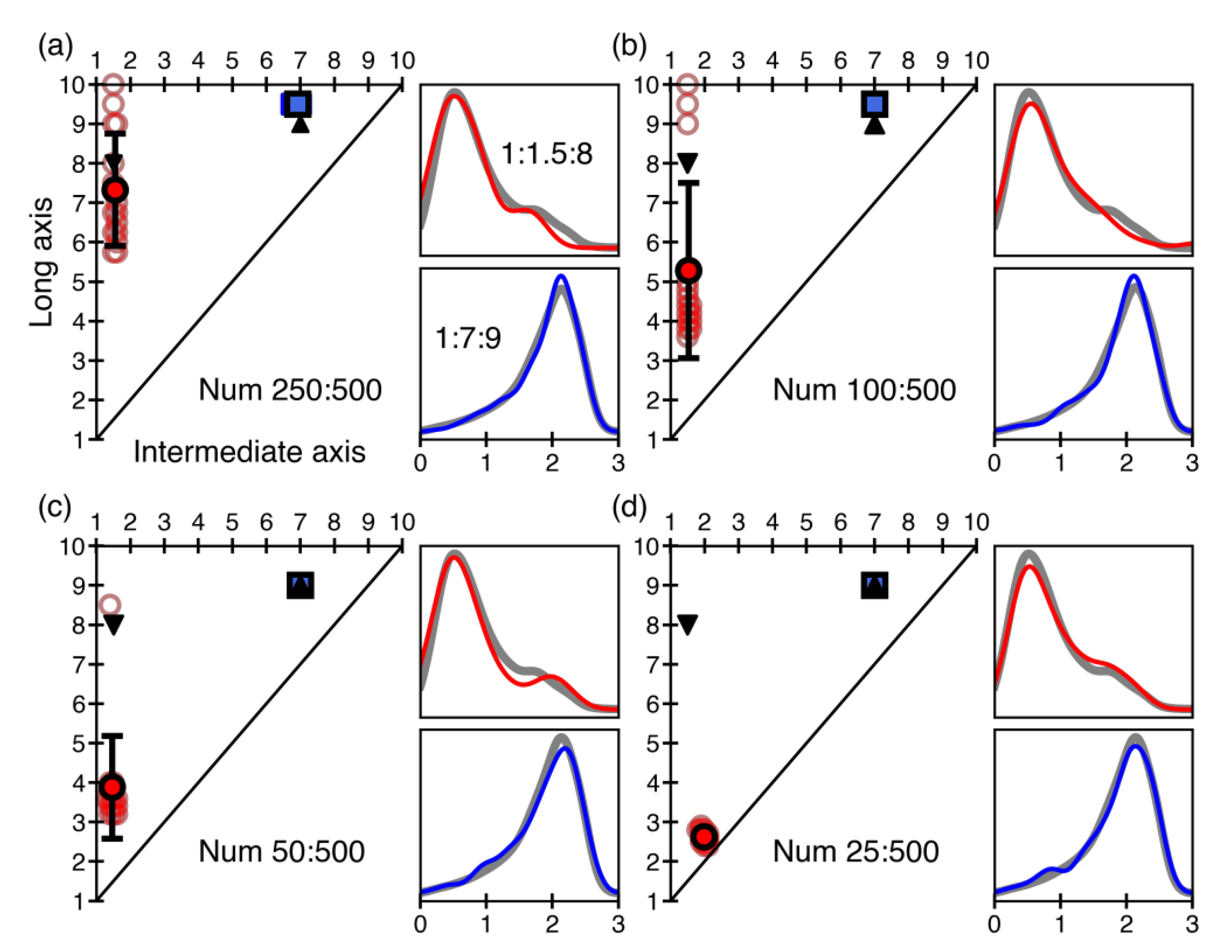
Figure 5), to verify the impact of the crystal number on the estimation. The other case is the end-members in different proportions. The dominant tabular habit has 500 crystals, and the crystal number of the prismatic habit ranges from 250 to 25 (Figure 6) to explore whether the model can distinguish a minority. We randomly select the 2D cut-sections of the two habits and compose the simulated samples for estimation. The independent randomly picked sections are irrelevant to the averaged pre-set curve in the database; thus, they can be used as datasets to test the model.
In Figure 5, the model can give accurate results if the end-members match the pre-set habits well. The long axis of the prismatic habit is hard to estimate accurately and is easy to obfuscate by the other habit, as the long axis can be cut in a low probability. More than 200 crystals of the prismatic can give us a better result. The tabular habit, however, needs fewer crystals for a stable distribution. In Figure 5b,c, the red curve deviates from the gray one, but we can still obtain a precise intermediate axis, although the long axis is hard to estimate. The blue curve in Figure 5a also goes off the pre-set data, and the estimated blue square still shows a similar tabular habit not far from the up-pointing triangle. Thus, our model is not sensitive to the deviations from pre-set habits. The results are acceptable when the end-members are roughly similar to the pre-set habits, regardless of the details. However, the crystal number of an end-member should be large enough if more accurate estimations are needed.
Figure 6a–d, the proportions of the prismatic habit continuously decline, and the estimation results change to a cubic-like habit, with the long axis being negligible. The corner point on the right part of the distribution curve represents the long axis, and the main peak on the left represents the intermediate (the red point with the black edge in Figure 6d). With the weight of the prismatic habit decreasing, the long axis is unlikely to estimate. For the ratios of 1:10 or 1:20 (Figure 6c,d), the prismatic habit has a smaller weight that can be ignored, but our model can still identify the main peak of the distribution, showing that multiple populations exist.
The above cases are mixtures of two habits. What if three or four populations of different habits exist in one sample? For example, plagioclase crystals first grow in tabular at low undercooling following prismatic crystals in the same batch of magma due to higher undercooling. After that, the magma containing crystals of tabular and prismatic habit injects into a chamber in which early formed crystals are equant. Thus, the final mixed magma contains crystals of the equant, tabular and prismatic. It is hard to find a natural sample meeting these ideal situations; thus, we use raw cut-sectional data of specific habits as above to test whether our model can identify mixed habits of three or four end-members. Considering an extreme situation where there are three habits in one sample, we assume that the mixed habits are composed of 1:1.5:2, 1:3:8 and 1:6:8, with their numbers of crystals at 100, 150, and 200, respectively, as an example to test our model. Two-dimensional sections of each habit are randomly generated by the cutting simulation, forming independent datasets irrelevant to the processed database. As illustrated in Figure 7a, the cubic habit of 1:1.5:2 is influenced largely by the flattened prismatic habit of 1:3:8, but the tabular habit is well estimated. This situation is unavoidable because the long axis of 3D crystal habit is hard to estimate. The habit 1:1.5:2 is similar to 1:3:8 in the intermediate axis, which is easy to confuse. Some crystals belonging to 1:3:8 are considered as a part of 1:1.5:2, yielding an incorrect estimation of 1:1.5:2. The intermediate axis of these three habits is well estimated. We then use the same three end-members whose crystal numbers are 600, 200, and 200, respectively, increasing the contents of 1:1.5:2 and 1:3:8 (Figure 7b). As expected, 1:1.5:2 and 1:3:8 with similar intermediate axes are still difficult to distinguish, and long axes are easily confused. However, the estimation of Figure 7b is far better than that of Figure 7a, indicating better distinction due to higher crystal numbers.
Technically, while complex mixed habits can be estimated by our enumerative method, the reliability of the results needs evaluating, especially mixed habits with similar intermediate axes, for their long axes are easily confused. This problem can be fixed if the long axis is accurately estimated by new methods or higher crystal numbers. However, accurate estimation of the long axis still remains unsolved from previous studies to our model. In this example, the accurate estimation of end-members with similar intermediate axes is difficult to achieve, due to indistinguishable long axes. Thus, after the estimation, we should evaluate whether the results are consistent with the petrographic observations.
In conclusion, HabitEst3D is not sensitive to external distractions. It can give acceptable estimations to the unknown sample, and the enumeration used in our model can identify end-members even with small weights. We should pay attention to estimating a mixture of more than three habits, especially those with similar intermediate axes, whose long axes are hard to estimate and are easily influenced by each other.

5. Example

We calculate the habit of clinopyroxene in the gabbroic sample named Z-6 from Panzhihua, Emeishan large igneous province [49]. The hand-traced outlines of clinopyroxene were processed by ImageJ [48] to ellipse fitting, and the sectional data are taken as an example in this study to test the program. In the 2D thin section of Sample Z-6, some of the clinopyroxene crystals are granular, but others are similar to the rectangular or elliptic with a higher aspect ratio (Figure 8a). Those sections with higher aspect ratios should belong to the short prismatic habit, which produces some granular sections due to the cut-section effect. According to the petrographic observation, we infer that there can be two populations, an isometric and a short prismatic habit. However, the values of these two habits are unknown and cannot be directly estimated from the 2D section.
We use the KDE method in HabitEst3D to estimate the crystal habit. In the single habit mode, the average of the top 15 results is 1:1.34 ± 0.1:1.91 ± 0.16, and the best-match result is 1:1.3:2 with RMSE = 0.12 (Figure 8b), which is an isometric–prismatic habit. The pre-set PDF does not fit the sample well, and RMSE is relatively high. The crystals in the sample may belong to multiple populations, consistent with the petrographic observation. We then use the multiple habits mode to explore the possible combinations of multiple habits in the sample (Figure 8c) with the number of habits set to two, and the top 15 results are selected. Those 15 results have RMSE values ranging from 0.016 to 0.022, two end-members are 33%–64% 1:1–2.1:2.4–2.9 and 36%–67% 1:1–1.4:1.4–1.8. One habit is isometric, and the other is mainly short prismatic but includes four thick tabular data. The result is common that the short prismatic and the thick tabular habits all have numbers of elongated sections, which is hard to identify when the number of crystals is small. The top five results with the lowest RMSE values have a narrow range of RMSE from 0.016 to 0.019, indicating that the results are similar. The best-match habit is 51% 1:1.2:2.8 with 49% 1:1.3:1.8, and the average calculated by hand is 55% 1:1.28 ± 0.15:2.7 ± 0.07 with 45% 1:1.28 ± 0.13:1.68 ± 0.13. Thus, we can conclude that the habits in the sample are composed of the short prismatic and the isometric, although the thick tabular data in some combinations are hard to filter out, which may be offset due to higher RMSE values. The results by the multiple habit mode are more reasonable because the simulated curve of mixed crystal habits fits the unknown PDF well, much better than the single habit estimation. In natural samples, the habits of crystals are commonly complex. If two or more habits exist in the sample, we can use the program to explore possible habit combinations close to the real one when one single habit deviates from the sample PDF.
Sample Z-6 consists of two similar habits. Here, we use another example containing two different types of oxide habits to test whether our model can distinguish between isometric and elongated 2D shapes. An example of a basaltic sample FS-16 [50] is illustrated in Figure 9 with a petrographic photo and hand-traced outlines of oxide. The total number of hand-traced oxide crystals is 1011, large enough to avoid uncertainties brought by smaller crystal numbers. We observe that oxide has elliptical and elongated 2D sections (Figure 9a,b), probably two populations of different habits in the sample. In Figure 9c, two tails of the sample and the estimated result do not fit well, indicating that the estimated long axis is inaccurate. In Figure 9d, the estimation by multiple habits mode and the sample overlap well with RMSE = 0.013, showing an accurate estimation. Our method can also give a good fit of a mixture of isometric and prismatic habits.

6. Discussion

Statistical methods for estimating true crystal habit in igneous rocks from 2D cut-sections have been developed for a long time. Higgins [15] used mathematical expressions, and Garrido, Kelemen and Hirth [14] used a diagram to estimate 3D habit. These statistical parameters generated by cutting simulations are fast and easy to explore regarding true crystal habits, but they may have larger errors when multiple crystal populations exist. The distributions of these cut-sections change regularly as the 3D habits vary, but these non-parametric complex distributions are hard to describe accurately only by some statistical parameters. Morgan and Jerram [16] used pre-set distributions to match the unknown sample and found the best-fit habit. The raw distribution curve is a direct mapping of cut-sections. However, it ignores the rules of statistics, and comparing the pre-set PDFs with the sample is an accurate method if the database is strong enough.
Based on previous studies, we use the pre-set habits and enumerate combinations to find the best-fit results, filling up the unknown curve with pre-set habits. In natural samples, multiple crystal populations with different habits may exist under changing environments or magma mixing. Previous methods cannot deal with multiple habits unless the mixed crystal populations can be separated manually. Our model finds possible end-members in a sample. The accuracy of the model depends on whether the sample meets the assumption. The database used in our study is built from random cut-sections of arbitrarily oriented cuboids. Thus, the estimation may have errors if the crystals or grains are rounded or foliated. Tabular and prismatic habits are easily influenced by magma flow. The distribution curve of oriented crystals is then changed, and a sharp peak may appear due to the fixed orientation of cut-sections. How the orientation affects the distribution curves remains unknown, including in previous studies related to 3D habit estimation. In this study, we performed simulations of randomly oriented cut-sections; thus, uncertain errors may occur if a sample is strongly affected by magma flow, which cannot be solved in our current model. The relationship between orientation and the distribution curve needs further careful quantitative evaluation. Therefore, we do not recommend using our current model in oriented samples. For further use applicable to oriented samples, a new database that fits the situation must be rebuilt to obtain more accurate estimations, and the whole procedure applied in the software can remain unchanged. In applications, our model can explore possible end-members of mixed crystal habits from 2D thin sections, indicating information on magma processes or crystallization dynamics [11,16,24].
Since we have discussions on estimating multiple habits, we need to find a threshold to distinguish multiple habits in a sample. Although previous studies give thresholds [16,24] to determine whether the estimation is good or not, it is still hard to choose an RMSE value to distinguish the existence of multiple habits as a threshold because RMSE is influenced by crystal number or habit types. In general applications, with the KDE method, RMSE equal to 0.015 indicates a good fit, and mixed crystal habits need to consider if RMSE is higher than 0.025. Higher RMSE occurs when the crystal number is smaller, for example, the threshold of 250 crystals mentioned previously [11,16]. In this case, RMSE higher than 0.05 indicates a poor fit with multiple habits in one sample. For the histogram method, RMSE higher than 0.15 indicates mixed crystal habits. There is another method to assess the goodness of fit qualitatively, whether or not the sample curve and the estimated result have similar trends or two curves that overlap well. The estimation by the KDE is more accurate than that by the histogram, so we recommend the KDE method for habit estimation.
Moreover, the average of these results is closer to the true habit, which is worth considering to reduce errors. As for multiple crystal populations, the model enumerates every possible combination to find the best-fit results. Logically, each pre-set habit has an equal chance of matching the unknown sample, but the key point is that the dominant habit covers some features of other habits with fewer crystals. The true habits can also appear in the results but may not within the top best-match ones. Cluster analyses such as k-means clustering [51] can be applied to the results to introduce different main types, which play a role similar to the average. Cluster analysis is more convenient to reveal the main types, but we did not add this function to our software, for it is better to analyze the results supervised. Single habit estimation can use the average or cluster to obtain a stable result, but estimation for multiple habits is complex. The results of different end-members surround the true value but may gather together to form an accidental cluster if the end-members are close, influencing the final types when applying cluster analysis. Until now, we have not come up with a better solution to apply cluster analysis to the estimation results, avoiding improper clusters. Thus, we suggest that the users take the first few results for further analysis, in consideration of petrographic observations and specific 2D sections. Additionally, applying cluster or average to estimation abandons the weights of the results, for only specific results belonging to one estimation can be combined to restore the unknown sample, but the clusters do not meet the requirements.
The essence of our model is an unmixing problem that solves end-members with their weights. Many statistical or machine-learning-based methods have been applied to this series of questions. As for our study, we cannot find a suitable solution by machine-learning or statistical methods, because the end-members will not be determined easily. We generate a database covering a wide range of pre-set habits, and there are small differences between the habits, similar to each other. The machine-learning or statistical methods are unable to decompose the unknown sample data to valid end-members. In comparison to Gaussian mixture models, end-members are Gaussian distributions that can be obtained by the expectation–maximization algorithm. However, in our model, the end-members are non-parametric and are unrelated to the statistical parameters. Thus, the machine-learning or statistical methods are not suitable for our model to find the right end-members. Thus we use the enumerative method to find the best-fit result, not the machine-learning methods.

7. Conclusions

HabitEst3D, based on our model proposed in this paper, is an easy-to-use cross-platform software with a user-friendly GUI to estimate the statistical crystal habit or to explore the possible habit combinations from 2D sectional data of an igneous sample by comparing with the pre-set data in a histogram or KDE. HabitEst3D reads the sectional data from the spreadsheet and performs logarithmic transformation for calculation. The program compares the sample data with the pre-set habits to find the best-fit results. When identifying mixed crystal habits, the program tries every possible combination and finds the estimation fitting with the sample. After the calculation, the program visualizes the results, and the user can save the data in versatile formats. The program is flexible, and when the sample does not meet the prerequisites, the user can compile a new database to fit the actual situation for more accurate estimations, with the whole process unchanged. Our model is robust to resist disturbances and can still have acceptable results even if the end-members with small weights go off the pre-set habits. The method introduced in this study is time-consuming but effectively explores mixed habits to investigate magma processes better. HabitEst3D is written in Python source code without compiling or packaging; thus, the users can easily modify or expand the program for more applications as they need.

Author Contributions

Conceptualization, methodology, writing—original draft preparation, J.L.; writing—review and editing, supervision, funding acquisition, Z.-F.Y.; writing—review and editing, supervision, Y.W. All authors have read and agreed to the published version of the manuscript.

Funding

This research was funded by the National Natural Science Foundation of China (92162213) and the Fundamental Research Funds for the Central Universities (2652019049; 2-9-2019-049).

Institutional Review Board Statement

Not applicable.

Informed Consent Statement

Not applicable.

Data Availability Statement

The Python program HabitEst3D based on this study can be found online: github.com/lj201112/HabitEst3D (accessed on 18 June 2022).

Acknowledgments

The authors thank the two anonymous reviewers for constructive comments on the manuscript, and the editor Aleksandra Milićev for meticulously and patiently processing the manuscript. Ye Yuan, Yahui Shen, and Rui Quan are appreciated for advice on the software.

Conflicts of Interest

The authors declare no conflict of interest.

References

  1. Donaldson, C.H. An experimental investigation of olivine morphology. Contrib. Mineral. Petrol. 1976, 57, 187–213. [Google Scholar] [CrossRef]
  2. Hammer, J.E.; Rutherford, M.J. An experimental study of the kinetics of decompression-induced crystallization in silicic melt. J. Geophys. Res. Solid Earth 2002, 107, ECV 8-1–ECV 8-24. [Google Scholar] [CrossRef]
  3. Higgins, M.D.; Chandrasekharam, D. Nature of Sub-volcanic Magma Chambers, Deccan Province, India: Evidence from Quantitative Textural Analysis of Plagioclase Megacrysts in the Giant Plagioclase Basalts. J. Petrol. 2007, 48, 885–900. [Google Scholar] [CrossRef] [Green Version]
  4. Lofgren, G.E. An experimental study of plagioclase crystal morphology: Isothermal crystallization. Am. J. Sci. 1974, 274, 243–273. [Google Scholar] [CrossRef]
  5. Lofgren, G.E. Experimental studies on the dynamic crystallization of silicate melts. In Physics of Magmatic Processes; Hargraves, R.B., Ed.; Princeton University Press: Princeton, NJ, USA, 1980; pp. 487–551. [Google Scholar]
  6. Higgins, M.D. Measurement of crystal size distributions. Am. Mineral. 2000, 85, 1105–1116. [Google Scholar] [CrossRef]
  7. Higgins, M.D. Closure in crystal size distributions (CSD), verification of CSD calculations, and the significance of CSD fans. Am. Mineral. 2002, 87, 171–175. [Google Scholar] [CrossRef]
  8. Jerram, D.A.; Higgins, M.D. 3D Analysis of Rock Textures: Quantifying Igneous Microstructures. Elements 2007, 3, 239–245. [Google Scholar] [CrossRef]
  9. Baker, D.R.; Mancini, L.; Polacci, M.; Higgins, M.D.; Gualda, G.A.R.; Hill, R.J.; Rivers, M.L. An introduction to the application of X-ray microtomography to the three-dimensional study of igneous rocks. Lithos 2012, 148, 262–276. [Google Scholar] [CrossRef]
  10. Godel, B. High-Resolution X-Ray Computed Tomography and Its Application to Ore Deposits: From Data Acquisition to Quantitative Three-Dimensional Measurements with Case Studies from Ni-Cu-PGE Deposits. Econ. Geol. 2013, 108, 2005–2019. [Google Scholar] [CrossRef]
  11. Mock, A.; Jerram, D.A. Crystal Size Distributions (CSD) in Three Dimensions: Insights from the 3D Reconstruction of a Highly Porphyritic Rhyolite. J. Petrol. 2005, 46, 1525–1541. [Google Scholar] [CrossRef]
  12. Cashman, K.V.; Marsh, B.D. Crystal size distribution (CSD) in rocks and the kinetics and dynamics of crystallization II: Makaopuhi lava lake. Contrib. Mineral. Petrol. 1988, 99, 292–305. [Google Scholar] [CrossRef]
  13. Higgins, M.D. Numerical modeling of crystal shapes in thin sections: Estimation of crystal habit and true size. Am. Mineral. 1994, 79, 113–119. [Google Scholar]
  14. Garrido, C.J.; Kelemen, P.B.; Hirth, G. Variation of cooling rate with depth in lower crust formed at an oceanic spreading ridge: Plagioclase crystal size distributions in gabbros from the Oman ophiolite. Geochem. Geophys. Geosyst. 2001, 2, 2000GC000136. [Google Scholar] [CrossRef]
  15. Higgins, M.D. Quantitative Textural Measurements in Igneous and Metamorphic Petrology; Cambridge University Press: Cambridge, UK, 2006; p. 265. [Google Scholar]
  16. Morgan, D.J.; Jerram, D.A. On estimating crystal shape for crystal size distribution analysis. J. Volcanol. Geotherm. Res. 2006, 154, 1–7. [Google Scholar] [CrossRef]
  17. Basu Sarbadhikari, A.; Day, J.M.D.; Liu, Y.; Rumble, D.; Taylor, L.A. Petrogenesis of olivine-phyric shergottite Larkman Nunatak 06319: Implications for enriched components in martian basalts. Geochim. Cosmochim. Acta 2009, 73, 2190–2214. [Google Scholar] [CrossRef]
  18. Jerram, D.A.; Mock, A.; Davis, G.R.; Field, M.; Brown, R.J. 3D crystal size distributions: A case study on quantifying olivine populations in kimberlites. Lithos 2009, 112, 223–235. [Google Scholar] [CrossRef]
  19. Martin, V.M.; Holness, M.B.; Pyle, D.M. Textural analysis of magmatic enclaves from the Kameni Islands, Santorini, Greece. J. Volcanol. Geotherm. Res. 2006, 154, 89–102. [Google Scholar] [CrossRef]
  20. Blundy, J.; Cashman, K. Petrologic Reconstruction of Magmatic System Variables and Processes. Rev. Mineral. Geochem. 2008, 69, 179–239. [Google Scholar] [CrossRef]
  21. Ruprecht, P.; Bergantz, G.W.; Cooper, K.M.; Hildreth, W. The Crustal Magma Storage System of Volcán Quizapu, Chile, and the Effects of Magma Mixing on Magma Diversity. J. Petrol. 2012, 53, 801–840. [Google Scholar] [CrossRef]
  22. Vinet, N.; Higgins, M.D. Magma Solidification Processes beneath Kilauea Volcano, Hawaii: A Quantitative Textural and Geochemical Study of the 1969–1974 Mauna Ulu Lavas. J. Petrol. 2010, 51, 1297–1332. [Google Scholar] [CrossRef] [Green Version]
  23. Kirkpatrick, R.J.; Klein, L.; Uhlmann, D.R.; Hays, J.F. Rates and processes of crystal growth in the system anorthite-albite. J. Geophys. Res. Solid Earth 1979, 84, 3671–3676. [Google Scholar] [CrossRef]
  24. Mangler, M.F.; Humphreys, M.C.S.; Wadsworth, F.B.; Iveson, A.A.; Higgins, M.D. Variation of plagioclase shape with size in intermediate magmas: A window into incipient plagioclase crystallisation. Contrib. Mineral. Petrol. 2022, 177, 64. [Google Scholar] [CrossRef]
  25. Muncill, G.E.; Lasaga, A.C. Crystal-growth kinetics of plagioclase in igneous systems; one-atmosphere experiments and application of a simplified growth model. Am. Mineral. 1987, 72, 299–311. [Google Scholar]
  26. Watanabe, K.; Kitamura, M. Growth mechanisms of plagioclase in a basaltic melt. Mineral. J. 1992, 16, 201–214. [Google Scholar] [CrossRef] [Green Version]
  27. Duchêne, S.P.; Pupier, E.; de Veslud, C.L.C.; Toplis, M.J. A 3D reconstruction of plagioclase crystals in a synthetic basalt. Am. Mineral. 2008, 93, 893–901. [Google Scholar] [CrossRef]
  28. Pupier, E.; Duchene, S.; Toplis, M. Experimental quantification of plagioclase crystal size distribution during cooling of a basaltic liquid. Contrib. Mineral. Petrol. 2008, 155, 555–570. [Google Scholar] [CrossRef]
  29. Shea, T.; Hammer, J.E. Kinetics of cooling- and decompression-induced crystallization in hydrous mafic-intermediate magmas. J. Volcanol. Geotherm. Res. 2013, 260, 127–145. [Google Scholar] [CrossRef]
  30. Cheng, L.; Costa, F. Statistical analysis of crystal populations and links to volcano deformation for more robust estimates of magma replenishment volumes. Geology 2019, 41, 1171–1175. [Google Scholar] [CrossRef]
  31. Zhu, Y.-X.; Wang, L.-X.; Ma, C.-Q.; Zhang, C. A flower-like glomerophyric diorite porphyry from Central China: Constraints on the unusual texture. Lithos 2018, 318–319, 1–13. [Google Scholar] [CrossRef]
  32. Li, J.; Yang, Z.; Wang, Y.; Li, P.; Luo, Z. A new statistical method to estimate crystal shape from two-dimensional sections in igneous rocks. Am. Mineral. 2022. unpublished (in revision) [Google Scholar]
  33. Scott, D.W. Multivariate Density Estimation: Theory, Practice, and Visualization, 1st ed.; John Wiley & Sons: New York, NY, USA, 1992; p. 317. [Google Scholar]
  34. Lascu, I.; Harrison, R.J.; Li, Y.; Muraszko, J.R.; Channell, J.E.T.; Piotrowski, A.M.; Hodell, D.A. Magnetic unmixing of first-order reversal curve diagrams using principal component analysis. Geochem. Geophys. Geosyst. 2015, 16, 2900–2915. [Google Scholar] [CrossRef] [Green Version]
  35. Weltje, G.J. End-member modeling of compositional data: Numerical-statistical algorithms for solving the explicit mixing problem. Math. Geol. 1997, 29, 503–549. [Google Scholar] [CrossRef]
  36. Dietze, E.; Hartmann, K.; Diekmann, B.; Ijmker, J.; Lehmkuhl, F.; Opitz, S.; Stauch, G.; Wünnemann, B.; Borchers, A. An end-member algorithm for deciphering modern detrital processes from lake sediments of Lake Donggi Cona, NE Tibetan Plateau, China. Sediment. Geol. 2012, 243–244, 169–180. [Google Scholar] [CrossRef]
  37. Weltje, G.J.; Prins, M.A. Muddled or mixed? Inferring palaeoclimate from size distributions of deep-sea clastics. Sediment. Geol. 2003, 162, 39–62. [Google Scholar] [CrossRef]
  38. Paterson, G.A.; Heslop, D. New methods for unmixing sediment grain size data. Geochem. Geophys. Geosyst. 2015, 16, 4494–4506. [Google Scholar] [CrossRef] [Green Version]
  39. Lee, D.D.; Seung, H.S. Learning the parts of objects by non-negative matrix factorization. Nature 1999, 401, 788–791. [Google Scholar] [CrossRef]
  40. Bro, R.; De Jong, S. A fast non-negativity-constrained least squares algorithm. J. Chemom. 1997, 11, 393–401. [Google Scholar] [CrossRef]
  41. Boutsidis, C.; Drineas, P. Random projections for the nonnegative least-squares problem. Linear. Algebra. Appl. 2009, 431, 760–771. [Google Scholar] [CrossRef] [Green Version]
  42. Harris, C.R.; Millman, K.J.; van der Walt, S.J.; Gommers, R.; Virtanen, P.; Cournapeau, D.; Wieser, E.; Taylor, J.; Berg, S.; Smith, N.J. Array programming with NumPy. Nature 2020, 585, 357–362. [Google Scholar] [CrossRef] [PubMed]
  43. Millman, K.J.; Aivazis, M. Python for Scientists and Engineers. Comput. Sci. Eng. 2011, 13, 9–12. [Google Scholar] [CrossRef] [Green Version]
  44. Oliphant, T.E. Python for Scientific Computing. Comput. Sci. Eng. 2007, 9, 10–20. [Google Scholar] [CrossRef] [Green Version]
  45. McKinney, W. Data structures for statistical computing in python. In Proceedings of the 9th Python in Science Conference, Austin, TX, USA, 28 June–3 July 2010. [Google Scholar]
  46. Hunter, J.D. Matplotlib: A 2D Graphics Environment. Comput. Sci. Eng. 2007, 9, 90–95. [Google Scholar] [CrossRef]
  47. Lam, S.K.; Pitrou, A.; Seibert, S. Numba: A LLVM-based Python JIT compiler. In Proceedings of the Second Workshop on the LLVM Compiler Infrastructure in HPC, Austin, TX, USA, 15 November 2015. [Google Scholar]
  48. Schneider, C.A.; Rasband, W.S.; Eliceiri, K.W. NIH Image to ImageJ: 25 years of image analysis. Nat. Meth. 2012, 9, 671–675. [Google Scholar] [CrossRef]
  49. Li, J.; Luo, Z.; Yang, Z.; Li, X.; Cheng, J.; Qiu, Y.; Vikentyev, I.V. The genesis of layered iron bodies occurring in the middle zone of Panzhihua intrusion, Zhujiabaobao mine: Evidence from quantitative crystal textural analysis. Earth. Sci. Front. 2016, 23, 210–220, (In Chinese with English Abstract). [Google Scholar] [CrossRef]
  50. Li, J.; Yang, Z.-F.; Wang, Y.; Xu, F.; Jiang, Q. Magma storage, ascending time and the link between alkaline and tholeiitic Cenozoic basalts in Taihang Mountains, North China Craton: Evidence from crystal size distributions and geochemical data of the Fanshi basalts. Geol. J. 2022. unpublished (in revision) [Google Scholar]
  51. Hartigan, J.A.; Wong, M.A. A K-Means Clustering Algorithm. J. R. Stat. Soc. Ser. C Appl. Stat. 1979, 28, 100–108. [Google Scholar] [CrossRef]
Figure 1. Cut-sections of the cuboid (1:2:5) and the distributions represented by histogram and kernel density estimation. (a) The simulated cuboid (1:2:5) representing a 3D crystal habit. (b) Random cut-sections of the cuboid. (c) The ln(AR) distribution of cut-sections represented by the histogram. (d) The ln(AR) distribution of cut-sections represented by the KDE. Ln(AR) is the logarithmic aspect ratio of the fitting ellipse of a cut-section. S, I, L represent the short, the intermediate, and the long axes, respectively.
Minerals 12 01001 g001
Figure 2. Flowcharts summarizing the algorithms for (a) single habit estimation and (b) mixed habits estimation. In the figure, N is the number of results to output, J is the loop times, AR represents the aspect ratio, and OLS represents the ordinary least squares.
Minerals 12 01001 g002
Figure 3. Interfaces of (a) single habit mode, (b) multiple habits mode, and (c) visualization of estimated results.
Minerals 12 01001 g003
Figure 4. Flowcharts showing the workflows for the estimation of (a) the single habit and (b) the mixed habits.
Minerals 12 01001 g004
Figure 5. Estimation results of the mixed habits of the prismatic and the tabular in the same proportion. The end-member habits are 1:1.5:8 (down-pointing triangle) and 1:7:9 (up-pointing triangle), representing the prismatic and the tabular, respectively. The top 15 results with the smallest RMSE values are selected, the red circles and the blue squares in the triangle plots represent the estimated prismatic and tabular habits, respectively, and those symbols with solid boundaries are the average with one standard deviation. To the right of the triangle plots are the distribution curves by KDE of the randomly picked cut-sections of the prismatic (1:1.5:8, red curve) and the tabular (1:7:9, blue curve) habits, and the gray curves are the end-members in the database. The ratios of crystal numbers of the prismatic to the tabular habit are (a) 25:25, (b) 50:50, (c) 100:100, (d) 200:200.
Minerals 12 01001 g005
Figure 6. Estimation results of mixed habits in different proportions. The ratios of crystal numbers of the prismatic to the tabular habit are (a) 250:500, (b) 100:500, (c) 50:500 and (d) 25:500. The legends and symbols in the figure are the same in Figure 5.
Minerals 12 01001 g006
Figure 7. Estimations of mixed habits. The end-members are 1:1.5:2, 1:3:8 and 1:6:8, and their crystal numbers are (a) 100, 150 and 200 (b) 600, 200 and 200, respectively. The blue square and the red circle represent the estimation result with minimal RMSE and the source data, respectively.
Minerals 12 01001 g007
Figure 8. Estimating the 3D habit from a natural sample. (a) Hand-traced outlines of clinopyroxene from the thin section (adapted with permission from Ref. [49]. 2016, Jie Li). The distributions of the sample and the estimated results using (b) single habit mode and (c) multiple habits mode are represented by KDE.
Minerals 12 01001 g008
Figure 9. Estimating the 3D habit of oxide from a natural basaltic sample. (a) Petrographic photo in reflected light [50]. (b) Hand-traced outlines of oxide (adapted with permission from Ref. [50]. 2022, Jie Li). The scale bar represents 200 μm. (c) Estimation by single habit mode. (d) Estimation by multiple habits mode.
Minerals 12 01001 g009
Publisher’s Note: MDPI stays neutral with regard to jurisdictional claims in published maps and institutional affiliations.

