
The Test Flight of iFTEM-I Fixed-Wing Airborne Time-Domain Electromagnetic System in Binxian, Heilongjiang Province, China

 and
and
Abstract
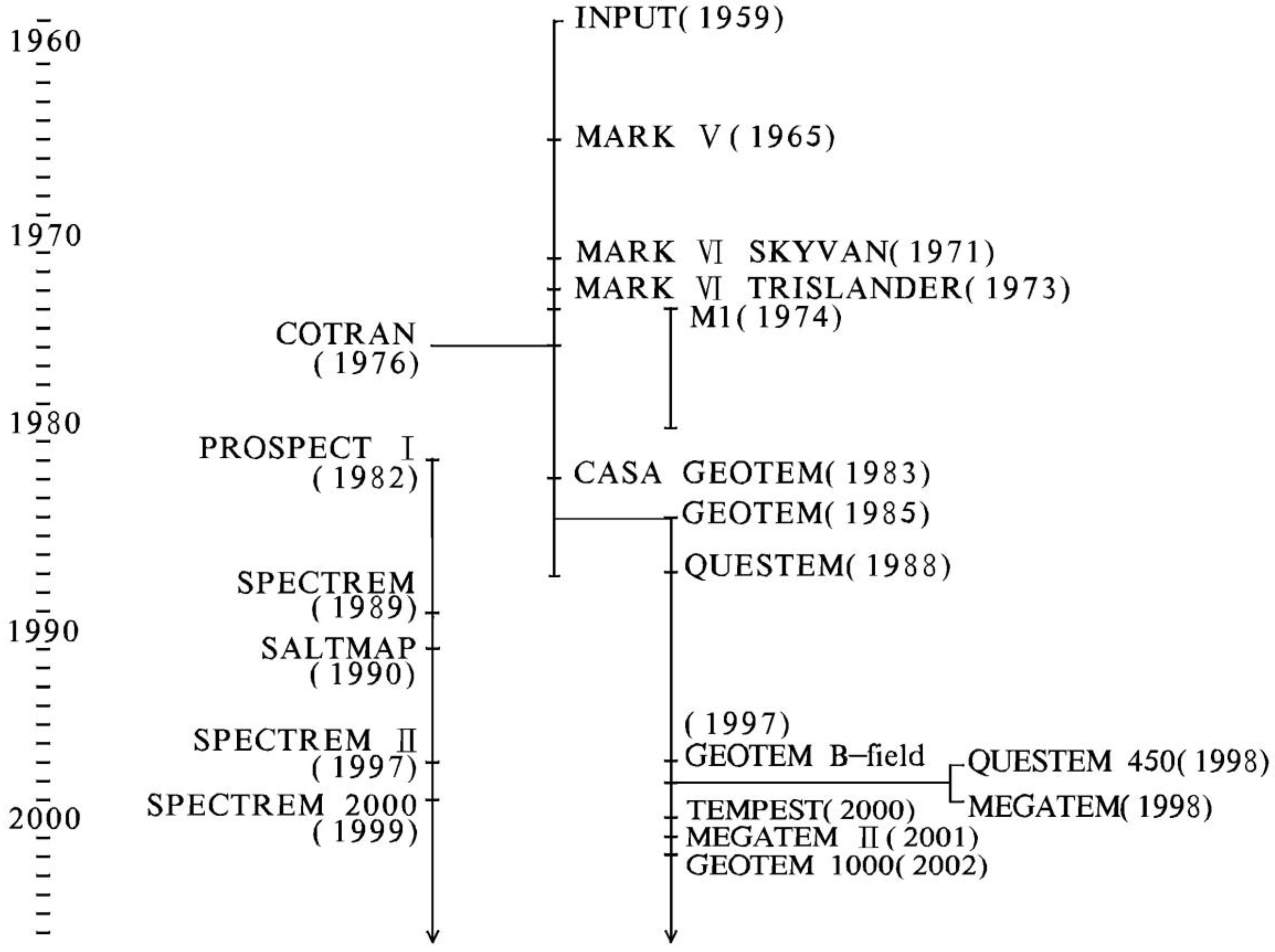
:1. Introduction
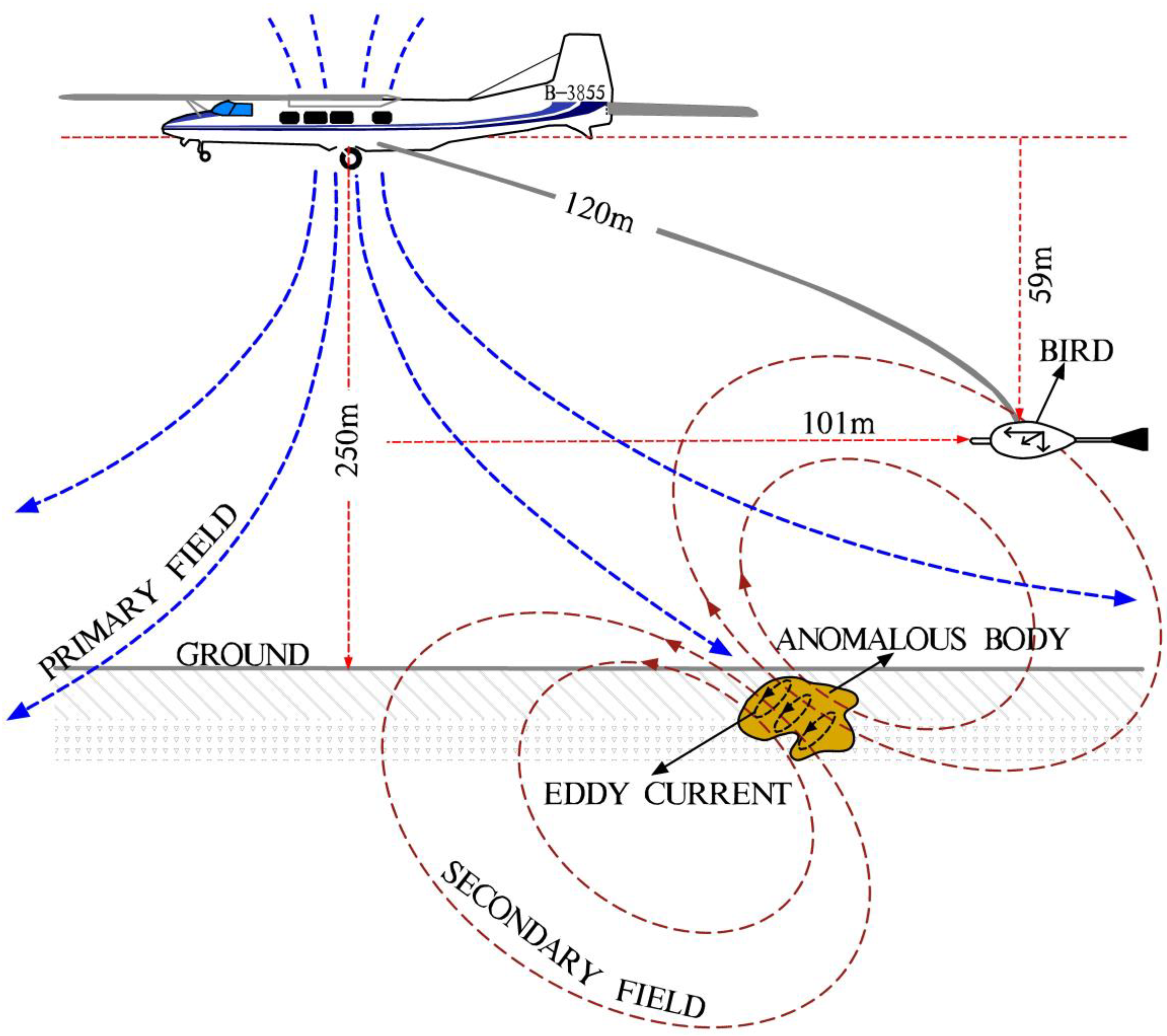
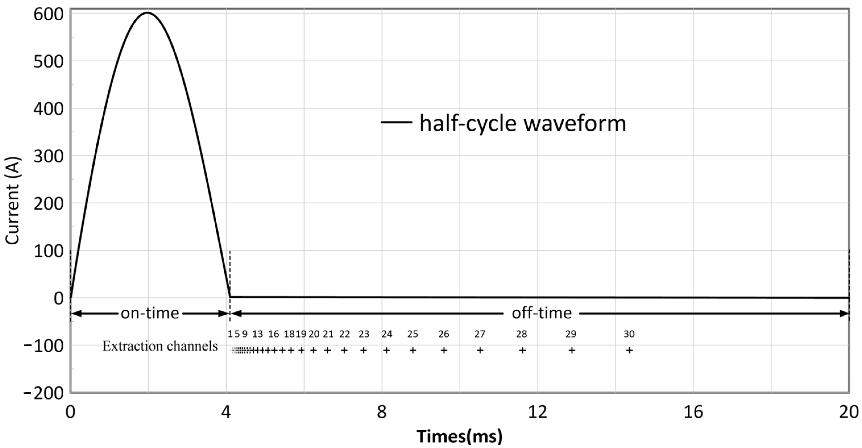
2. The iFTEM-I System
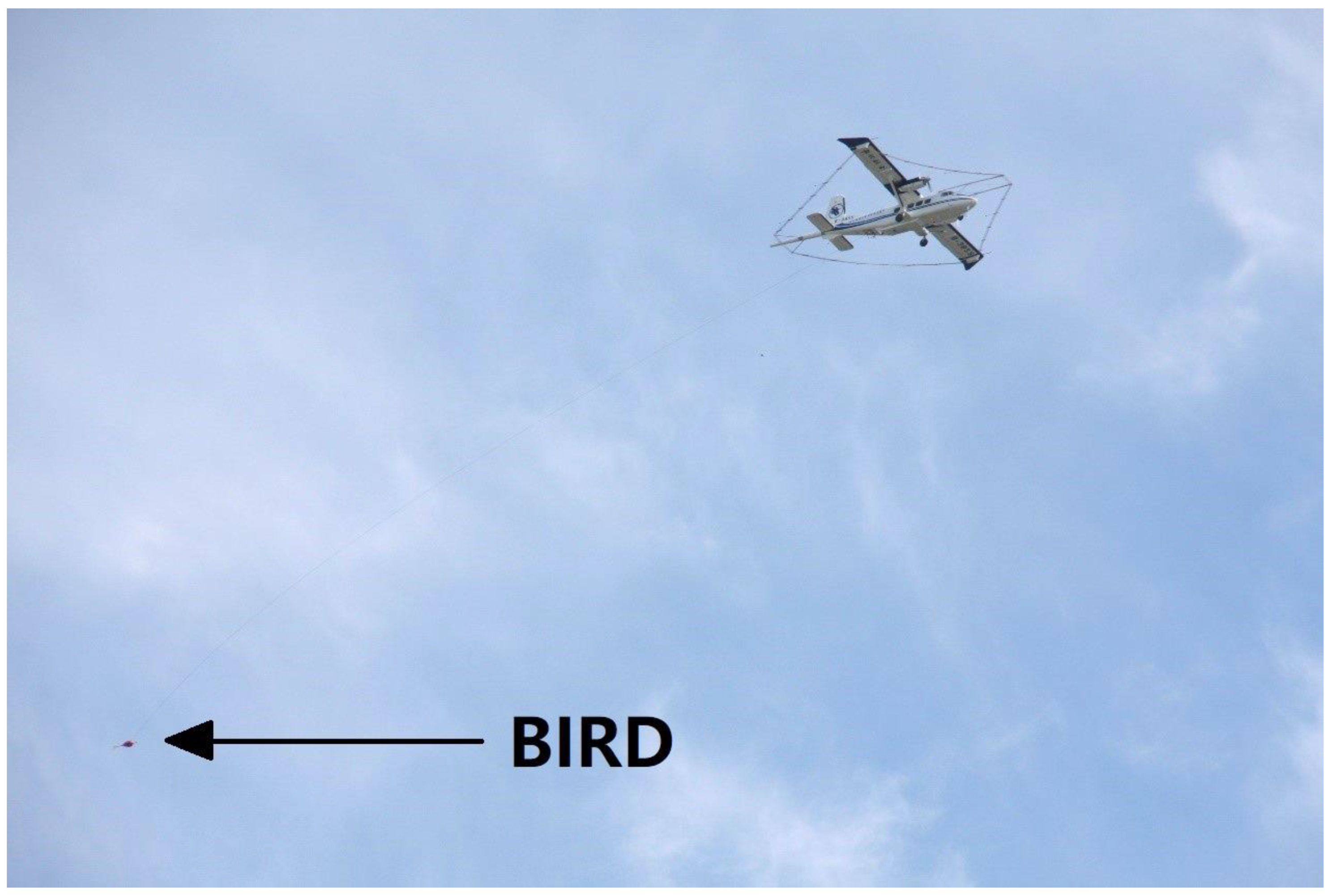
3. Survey Flight
3.1. Geological Setting
3.2. Survey Flight and Data Processing
3.3. Mapping
4. Ground TEM Survey
5. Results Comparison
6. Discussion
7. Conclusions
Author Contributions
Funding
Acknowledgments
Conflicts of Interest
References
- Ping, H.; Wenjie, L.; Junfeng, L.; Qingmin, M.; Xuben, W.; Xiaodong, C.; Yingying, L. The Advances in the Development of Fixed-Wing Airborne Time-Domain Electromagnetic System. Acta Geosci. Sin. 2012, 33, 7–12. (In Chinese) [Google Scholar] [CrossRef]
- Heath, P.; Dhu, T.; Keeping, T.; Reed, G.; Gouthas, G.; Katona, L.; Fairclough, M. A Review of AEM in South Australia. ASEG Ext. Abstr. 2013, 2013, 1–5. [Google Scholar] [CrossRef] [Green Version]
- Fountain, D. Airborne Electromagnetic Systems—50 Years of Development. Explor. Geophys. 1998, 29, 11. [Google Scholar] [CrossRef]
- Thomson, S.; Fountain, D.; Watts, T. Airborne Geophysics—Evolution and Revolution. 2007, pp. 19–37. Available online: https://vdocuments.net/airborne-geophysics-evolution-and-exploration-against-this-background-of.html?page=1 (accessed on 24 April 2022).
- Smith, R.; Fountain, D.; Allard, M. The MEGATEM Fixed-Wing Transient EM System Applied to Mineral Exploration: A Discovery Case History. First Break 2003, 21, 26–30. [Google Scholar] [CrossRef]
- Reed, L.E. The Airborne Electromagnetic Discovery of the Detour Zinc-copper-silver Deposit, Northwestern Québec. Geophysics 1981, 46, 1278–1290. [Google Scholar] [CrossRef]
- Leggatt, P.B.; Klinkert, P.S.; Hage, T.B. The Spectrem Airborne Electromagnetic System—Further Developments. Geophysics 2000, 65, 1976–1982. [Google Scholar] [CrossRef]
- Lane, R.; Green, A.; Golding, C.; Owers, M.; Pik, P.; Plunkett, C.; Sattel, D.; Thorn, B. An Example of 3D Conductivity Mapping Using the TEMPEST Airborne Electromagnetic System. Explor. Geophys. 2000, 31, 162–172. [Google Scholar] [CrossRef]
- Klinkert, P.S.; Leggatt, P.B.; Hage, T.B. The Spectrem Airborne Electromagnetic System—Latest Developments and Field Examples. Proc. Explor. 1997, 97, 557–564. [Google Scholar]
- King, A.; Roux, T.L. Spectrem2000 AEM as a Mapping and Discovery System. ASEG Ext. Abstr. 2007, 2007, 1–3. [Google Scholar] [CrossRef]
- Duncan, A.C.; Roberts, G.P.; Buselli, G.; Pik, J.P.; Williamson, D.R.; Roocke, P.A.; Thorn, R.G.; Anderson, A. SALTMAP—Airborne EM for the Environment. Explor. Geophys. 1992, 23, 123–126. [Google Scholar] [CrossRef]
- Annan, A.P.; Lookwood, R. An Application of Airborne Geotem in Australian Conditions. Explor. Geophys. 1991, 22, 5–12. [Google Scholar] [CrossRef]
- Changda, Z. Airborne Time Domain Electromagnetics System:Look Back and Ahead. Chin. J. Eng. Geophys. 2006, 3, 265–273. (In Chinese) [Google Scholar]
- Yue, Z.; Feng, X.; Xiu, L. Review on Time-Domain AEM System and Applied Potential. Prog. Geophys. 2017, 32, 2709–2716. (In Chinese) [Google Scholar] [CrossRef]
- Yin, C.-C.; Zhang, B.; Liu, Y.; Ren, X.; Qi, Y.-F.; Yifeng, P.; Qiu, C.; Huang, X.; Huang, W.; Jiajia, M.; et al. Review on Airborne EM Technology and Developments. Chin. J. Geophys. 2015, 58, 2637–2653. (In Chinese) [Google Scholar] [CrossRef]
- Annan, A.P. Benefits Derived from the Use of a Fully Digital Transient Airborne EM System. In Proceedings of the SEG Technical Program Expanded Abstracts 1990, San Francisco, CA, USA, 23–27 September 1990; pp. 693–695. [Google Scholar]
- Wynn, J. Evaluating Groundwater in Arid Lands Using Airborne Magnetic/EM Methods: An Example in the Southwestern U.S. and Northern Mexico. Lead. Edge 2002, 21, 62–64. [Google Scholar] [CrossRef]
- Wolfgram, P.; Golden, H. Airborne EM Applied to Sulphide Nickel—Examples and Analysis. ASEG Ext. Abstr. 2001, 34, 136–140. [Google Scholar] [CrossRef]
- Witherly, K.; Sattel, D. An Assessment of Geotem, Falcon ® and ZTEM Surveys over the Nebo Babel Deposit, Western Australia. ASEG Ext. Abstr. 2018, 2018, 1–7. [Google Scholar] [CrossRef] [Green Version]
- Witherly, K.; Diorio, P. Application of Airborne Magnetics, EM and Gravity to the Ring of Fire Intrusive Complex, Ontario. In Proceedings of the SEG Technical Program Expanded Abstracts 2014; Society of Exploration Geophysicists, Denver, Colorado, 5 August 2014; pp. 1704–1708. [Google Scholar]
- Vrbancich, J.; Wolfgram, P.; Sattel, D. AEM Bathymetry near Busselton, Western Australia—Comparison of 25 Hz and 12.5 Hz GEOTEM in Areas of High Conductance. ASEG Ext. Abstr. 2003, 2003, 1–4. [Google Scholar] [CrossRef]
- Vrbancich, J.; Macnae, J.; Sattel, D.; Wolfgram, P. A Case Study of AEM Bathymetry in Geographe Bay and over Cape Naturaliste, Western Australia, Part 2: 25 and 12.5 Hz GEOTEM. Explor. Geophys. 2005, 36, 381–392. [Google Scholar] [CrossRef]
- Smith, R.S.; Koch, R.; Hodges, G.; Lemieux, J. A Comparison of Airborne Electromagnetic Data with Ground Resistivity Data over the Midwest Deposit in the Athabasca Basin. Near Surf. Geophys. 2011, 9, 319–330. [Google Scholar] [CrossRef]
- Smith, R.S.; Koch, R. Airborne EM Measurements over the Shea Creek Uranium Prospect, Saskatchewan, Canada. In Proceedings of the SEG Technical Program Expanded Abstracts 2006; Society of Exploration Geophysicists: Houston, TX, USA, 2006; pp. 1263–1267. [Google Scholar]
- Smith, R.S.; Cheng, L.Z.; Chouteau, M. Using Reversed Polarity Airborne Transient Electromagnetic Data to Map Tailings around Mine Sites. Lead. Edge 2008, 27, 1470–1478. [Google Scholar] [CrossRef]
- Smith, R.S.; Annan, A.P.; Lemieux, J.; Pedersen, R.N. Application of a Modified GEOTEM System to Reconnaissance Exploration for Kimberlites in the Point Lake Area, NWT, Canada. Geophysics 1996, 61, 82–92. [Google Scholar] [CrossRef]
- Paine, J.G.; Collins, E.W. Applying Airborne Electromagnetic Induction in Ground-Water Salinization and Resource Studies, West; Society of Exploration Geophysicists: Houston, TX, USA, 2003. [Google Scholar]
- Dickinson, J.E.; Pool, D.R.; Groom, R.W.; Davis, L.J. Inference of Lithologic Distributions in an Alluvial Aquifer Using Airborne Transient Electromagnetic Surveys. Geophysics 2010, 75, WA149–WA161. [Google Scholar] [CrossRef] [Green Version]
- Cheng, L.Z.; Smith, R.S.; Allard, M.; Keating, P.; Chouteau, M.; Lemieux, J.; Vallée, M.A.; Bois, D.; Fountain, D.K. Evaluation of the Efficiency of Several Airborne Electromagnetic Systems. Explor. Min. Geol. 2009, 18, 12. [Google Scholar]
- Geotech Ltd. Evaluating Signal to Noise and Depth Investigation of Airborne Time. Available online: https://www.geotech.ca/documents/VTEM_SignaltoNoise.pdf (accessed on 3 April 2022).
- Grant, F.S.; West, G.F. Interpretation Theory in Applied Geophysics; McGraw-Hill Book Co.: New York, NY, USA, 1965; ISBN 978-0070241008. [Google Scholar]
- Zhili, X.; Wei, H.; Junjie, L.; Fei, L. Design and Implementation of Supporting Platform for Airborne Geophysical Exploration Software System. Comput. Tech. Geophys. Geochem. Explor. 2020, 42, 131–137. (In Chinese) [Google Scholar] [CrossRef]
- Qingquan, Z.; Junjie, W.; Xiaohong, D.; Jie, Z. The One-Dimension Inversion of Underground Transient Electromagnetic Data. Comput. Tech. Geophys. Geochem. Explor. 2015, 37, 566–570. (In Chinese) [Google Scholar] [CrossRef]
- Spies, B.R. Depth of Investigation in Electromagnetic Sounding Methods. Geophysics 1989, 54, 872–888. [Google Scholar] [CrossRef]


| Model | iFTEM-I | GEOTEM |
|---|---|---|
| Aircraft | Y12-IV | CASA-212 |
| Aircraft speed (km/h) | 230 | 400 |
| Peak transmitter dipole moment (Am2) | 504,000 | 690,000 |
| Transmitter waveform | half sine wave | half sine wave |
| Base frequency | 12.5, 25 | 12.5, 25 |
| Bandwidth | 0–20 | 0–10 |
| Data unit | dB/dt | dB/dt or dB |
| Noise level (nT/s) | 13 | 1–2 |
| Parameters | Values |
|---|---|
| Transmitter base frequency | 25 Hz |
| Transmitter height (VAGL 1) | 210 m |
| Receiver bird height (VAGL) | 151 m |
| Transmitter–bird horizontal separation | 101 m |
| Transmitter peak current | 600 A |
| Transmitter pulse width | 4.15 ms |
| Loop area | 210 m2 |
| Number of turns | 4 |
| Transmitter dipole moment | 504,000 Am2 |
| Equivalent receiver area | 19,000 m2 |
| Sampling rate | 100 kHz |
| Sampling bits | 24 bits |
| Data channels | Rv, Rz, Rx, Ry, Longitude, Latitude, GPS_time, GPS_Altitude, Radar_altitude |
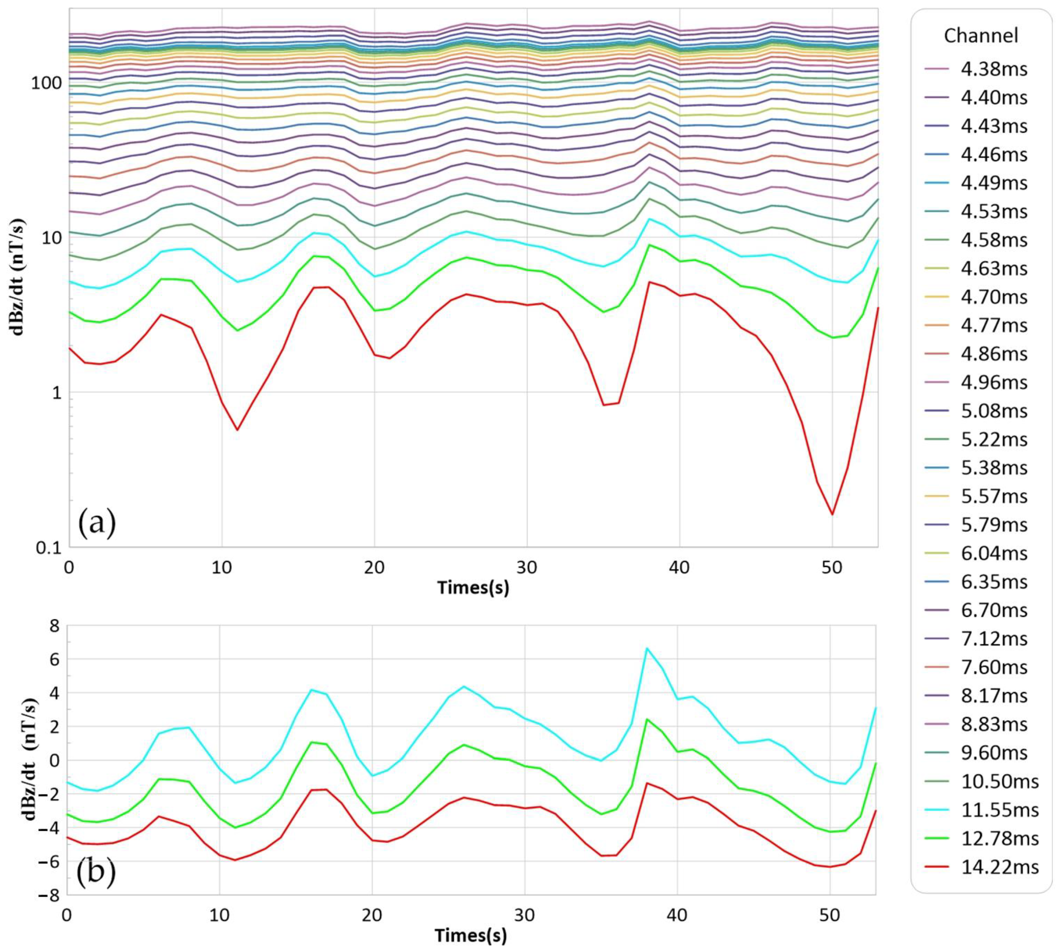
| Gate centers after on-time (post data processing) | 4.36, 4.38, 4.40, 4.43, 4.46, 4.49, 4.53, 4.58, 4.63, 4.70, 4.77, 4.86, 4.96, 5.08, 5.22, 5.38, 5.57, 5.79, 6.04, 6.35, 6.70, 7.12, 7.60, 8.17, 8.83, 9.60, 10.50, 11.55, 12.78, 14.22 ms |
Publisher’s Note: MDPI stays neutral with regard to jurisdictional claims in published maps and institutional affiliations. |
© 2022 by the authors. Licensee MDPI, Basel, Switzerland. This article is an open access article distributed under the terms and conditions of the Creative Commons Attribution (CC BY) license (https://creativecommons.org/licenses/by/4.0/).
Share and Cite
Zheng, H.; Li, J.; Huang, W.; Liu, Y.; Li, F.; Meng, Q.; Zhi, Q.; Wang, X.; Lu, N. The Test Flight of iFTEM-I Fixed-Wing Airborne Time-Domain Electromagnetic System in Binxian, Heilongjiang Province, China. Minerals 2022, 12, 890. https://doi.org/10.3390/min12070890
Zheng H, Li J, Huang W, Liu Y, Li F, Meng Q, Zhi Q, Wang X, Lu N. The Test Flight of iFTEM-I Fixed-Wing Airborne Time-Domain Electromagnetic System in Binxian, Heilongjiang Province, China. Minerals. 2022; 12(7):890. https://doi.org/10.3390/min12070890
Chicago/Turabian StyleZheng, Hongshan, Junfeng Li, Wei Huang, Yu Liu, Fei Li, Qingmin Meng, Qingquan Zhi, Xingchun Wang, and Ning Lu. 2022. "The Test Flight of iFTEM-I Fixed-Wing Airborne Time-Domain Electromagnetic System in Binxian, Heilongjiang Province, China" Minerals 12, no. 7: 890. https://doi.org/10.3390/min12070890
APA StyleZheng, H., Li, J., Huang, W., Liu, Y., Li, F., Meng, Q., Zhi, Q., Wang, X., & Lu, N. (2022). The Test Flight of iFTEM-I Fixed-Wing Airborne Time-Domain Electromagnetic System in Binxian, Heilongjiang Province, China. Minerals, 12(7), 890. https://doi.org/10.3390/min12070890