Metallic-Mineral Prospecting Using Integrated Geophysical and Geochemical Techniques: A Case Study from the Bela Ophiolitic Complex, Baluchistan, Pakistan

Abstract

An integrated geophysical and geochemical investigation was conducted to investigate the metallic minerals hosted in the mafic and ultramafic rocks in the Bela Ophiolitic Complex. Two thousand magnetic observations were made along with six vertical electrical soundings, with Induced Polarization (IP) targeting the anomalous magnetic zones. The magnetic raw field data were interpreted qualitatively and quantitatively, and two anomalous zones (A1 and A2) were identified on the magnetic maps. The residual magnetic values in the high-magnetic-anomalous zone (A2) ranged from 310 nT to 550 nT, while the magnetic signatures in the low-magnetic zone (A1) ranged from –190 nT to 50 nT. The high-anomalous zone (A2) was distinguished by a high IP value ranging from 3.5 mV/V to 15.1 mV/V and a low apparent and true resistivity signature of 50 ohm·m. Whereas, the low-anomalous zone (A1) was distinguished by very low IP values ranging from 0.78 mV/V to 4.1 mV/V and a very high apparent and true resistivity of 100 ohm·m. The Euler deconvolution was used to determine the depth of the promising zone, which for A1 and A2 was in the 100 m range. The statistical analysis was carried out using hierarchical classification to distinguish between background and anomalous data. The high-magnetic anomalous signature of probable mineralization was in the range of 46,181 nT–46,628 nT, with a total intensity range of 783 nT–1166 nT. The major and trace-element analysis of the 22 rock and stream sediments collected from the high-magnetic-anomalous zone confirmed the mineralization type. The geomagnetic and geophysical cross sections revealed that anomalous mineralization was concentrated with the anticlinal Bela Ophiolitic Complex. The generated results also aided in the identification of rock boundaries, depth, and hidden faults in the area. The findings revealed that the study area has excellent mineralization associated with the ultramafic-rock sequence.

1. Introduction

The Ophiolites play an important role in understanding plate tectonics, ocean floor composition, and earth evolution [1,2,3]. The ophiolite sequence constitutes exhumed oceanic lithosphere that contributes to economic mineralization [4,5,6]. The sequence offers promising prospects for metalliferous mineral enrichment, such as Fe, Cu, Au, Ag, Cu, Pb, Zn, Ni, and Cr [7,8,9,10]. The ophiolite succession in Pakistan was formed on the Neotethys ocean floor before the Late Cretaceous collision of the Eurasian–Indian plate [11,12]. The succession has been reported in several locations throughout Pakistan, ranging from the Karakorum–Himalaya region in the north to the Lasbela district in the south [12,13]. The northern margin of the country has been extensively studied, whereas the southwestern margin requires further research [14]. The SW margin is characterized by the Bela Ophiolitic Complex (BOC), Pakistan’s largest Ophiolitic belt located along the Indian–Asian boundary [13]. The BOC has a length of over 450 km and a width of 10 km, covered by alluvium in front of the Arabian Sea [14]. It is a dismembered sequence that was presumably formed as a single thrust sheet during the Eurasian–Indian orogeny [13,15]. The ophiolite is composed of serpentinized-mantle harzburgite-layered peridotite, gabbros, sheeted dykes, basaltic-pillow lava, and associated sedimentary rocks [13,14,16]. According to studies, BOC has the high economic potential of Fe, Mn, Ti, Cr, Ni, Co, Zn, and Pb [13,16,17,18,19,20]. The mafic and ultramafic sequences, aided by the BOC tectonic regime, demarcate economic potential host spots for metallogenic minerals [11,17,21]. Narejo et al. (2019) and Ali (1971) postulated hydrothermal Mn deposits of volcanogenic sedimentary origin, proposing a study that includes detailed deposit descriptions using a combination of geological and geophysical approaches [18,20]. The magnetic signature [13] (Zaigham, 1991) and aeromagnetic anomaly [22] (Canada, 1981) indicate that the BOC has excellent mineralization potential, but further investigation is needed.

Geomagnetic survey plays an important role in the mineral-resource mapping, geodynamic study, and tectonic evolution of any area [23,24,25]. Magnetic anomalies are initiated by two factors: data intensity and a strong physical contrast (e.g., magnetic susceptibility) between the target and host rocks. The high-magnetic anomalies are usually generated by ophiolites of great spatial extent, generated by the subducting plate along the suture zone [26], while intermediate and low-magnetic anomalies are observed in igneous rocks of small extent or local tectonic uplift [27].

This study is mainly focused on the exploration of metallic minerals hosted in mafic and ultramafic rocks of the BOC, based on the qualitative and quantitative analysis of field data for the magnetic and IP/resistivity targeting of the aeromagnetic anomaly [22]. A geophysical study on BOC was carried out for the first time to investigate the mineral potential. In addition, the mineralization type determined by the magnetic anomaly was confirmed by geochemical investigation of the rock and stream sediments samples. Figure 1 shows the studied region is a part of the Bela Ophiolitic band and is located between latitudes 26°00′02″ and 26°02′15″ E and longitudes 66°37′25″ and 66°41′06″ N, 20 km from Uthal, Lasbela District, Baluchistan, Pakistan. The lithological units exposed in the study area are Bela volcanic melange (Kbv), lava flow (Kbvs), Bela intrusive (Kbg), Aeolian sand (Qt), streambed deposits (Qaf), and Quaternary alluvium (Qs) [13].

2. Materials and Methods

Magnetic and IP/resistivity surveys were performed to identify mineralized zones, magnetic signatures, and geological settings in the study area. Geochemical analysis was carried out to validate the mineralization type and its potential.

2.1. Magnetic Data Acquisition

A detailed ground magnetic survey was carried out in a regular grid pattern of 50 m × 100 m intervals. The magnetic signature of the rocks was used to detect underlying geological features and economic deposits, with a total of 2000 geomagnetic sites covering a 25 km² area as presented in Figure 1 below. The proton precession magnetometer G-856 of Geometrics, USA, was used to conduct the magnetic survey, widely used for mineral exploration and subsurface mapping [28,29,30]. To eliminate the diurnal impact during the field survey, the base station was carefully selected by fixing one magnetometer, where the magnetic strengths were measured at a steady position. Two magnetometers were used to measure the total intensity of the magnetic field at each observation point along with the survey. To filter the raw data, the magnetic data were processed using computer software Oasis montaj 8.4 (Geosoft Europe Ltd., Wallingford, UK).

Processing and Interpretation of Magnetic Data

Since the Earth is an oblate spheroid with magnetic values ranging from 25,000 nT at the Equator to 65,000 nT at the poles, the magnetic data recorded were corrected for the influence of latitude [31]. At both the regional and base levels, latitude correction (L.C.) was applied. Using Oasis montaj, the regional L.C. was calculated by subtracting the obtained field data from the International Geomagnetic Reference Field (IGRF) [32]. Since the area has a high potential for mineralization of the Bela mafic sequence, the L.C. at the base level was used to reduce distortion at the local scale [13,16,17,18,20]. For Pakistan, the L.C. was calculated by subtracting the base north from the station north and multiplying the difference by the latitude factor constant (L.F.C.) of 0.0043/m. Concerning the base, the L.C. value changed from −21 nT/m to −39 nT/m.

2.2. Resistivity/IP Survey

The prospective zones demarcated by geomagnetic imprints were analyzed for sulfide mineralization using Vertical Electrical Sounding (VES) and Induced Polarization (IP) surveys. IRIS, Orly, France, and the TSQ-3 Transmitter by Scintrex, Concord, ON, Canada conducted the VES/IP survey using Elrec Pro (receiver). These instruments are having high sensitivity and a maximum depth of penetration for detailed analysis of the subsurface regime [33,34]. Both transmitter and receiver measurements were taken in the time domain with t = 2 s. The Schlumberger configuration was utilized to measure resistivity and IP along with three VESs in the NW–SE direction, with an electrode spacing of AB/2 = 10 m to 150 m and a potential MN = 2 m to 25 m. To calculate true resistivity with corresponding thickness and depth, the IPI2win program was used to invert resistivity data using forward-inversion techniques.

2.3. Geochemical Analysis

The geochemical analysis was carried out to verify the mineralization that was d lineated by the magnetic and VES/IP surveys. A total of 12 rock- and 10 stream-sediment samples were collected from the high-magnetic-anomalous zone. The samples were analyzed for major and trace elements using Panalytical Axios (Panalytical Ltd, Malvern, United Kingdom) Wavelength-Dispersive X-ray Fluorescence (WD-XRF), Model PW-4440, good for analyzing both major and minor elements [3]. The samples were ground to make them homogenous and then passed through a 200-mesh sieve. To record the loss on ignition (LOI), 1 g sample was oven-dried for 2 h at 1000 °C and any organic and carbonate materials were removed. The glass beads were made for major-element analysis by placing 0.5 g of oven-dried sample in a glass bead maker for 20 min and using 5 g of di-lithium tetra borate in a platinum crucible. The trace-element analysis was performed on dry-powder pellets.

3. Results

3.1. Magnetic

Figure 2a depicts a Total Magnetic Intensity (TMI) map with a contour interval of 10 nT, and geomagnetic readings normalized for diurnal changes. The diurnal correction was applied to compensate for the daily and seasonal variations in the geomagnetic field [34]. During the current investigation, the diurnal correction ranged from −6 nT to 15 nT, implying no magnetic secular variation [35].

The TMI changed from 44,920 nT to 46,130 nT, a difference of 1210 nT. According to the World Magnetic Model (2020), the regional background magnetic intensity value of the area is 45,000 nT, on which magnetometer G-856 is tuned to achieve the best signal results [36], whereas the average base-station magnetic measurement is 45,494 nT. The ultramafic and mafic sequences of Bela ophiolites are responsible for a total change of 494 nT [14]. Figure 2b shows the Total Magnetic Anomaly (TMA) map prepared by subtracting the base measurement from the TMI. The TMA value varied from −580 nT to 630 nT, implying a total change of 1210 nT; the TMI and TMA concur on this overall shift. Maximum TMA values varied from 320 nT to 620 nT, representing a total of 300 nT anomaly, with low-anomalous values positioned between −280 nT and −580 nT, representing a zone of −300 nT. The inclination and declination of the magnetic field distort the shape and size of magnetic anomalies [37]. This distortion effect was removed by processing the TMA map grid using a mathematical approach called Reduction to Pole (RTP) (depending on the latitude of the survey region and the dip angle of the magnetization vector in the body) [38]. Figure 2c shows the output as an RTP map, which is independent of the magnetic pole inclination and declination of geological bodies creating anomalies. The RTP raised the magnetic value by 400 nT at the maximum and 220 nT at the minimum, concerning the TMA map, resulting in a total magnetic value of −800 nT to 1030 nT. The field parameters of the study area used for RTP were: total field strength of 45,000 nT, magnetic declination of 1.10°, and magnetic inclination of 40.76°. The TMA was related to the high-intensity shift in the RTP map, which ranged 23 m from the west and 726 m from the south, with a 1500 m shift from the north and an 800 m shift from the south. Figure 2d shows the Residual Magnetic (RM) anomaly map, generated by subtracting regional magnetic values from the TMA map, resulting in a total magnetic range of −660 nT to 550 nT. The RM map indicates a decrease in magnetic value by 80 nT of TMA and 480 nT of RTP at the maximum and a drop in magnetic value by −80 nT of TMA and −140 nT of RTP at the minimum. The magnetic value of TMA is higher than that of RMA due to the mafic and ultramafic sequences of BOC [12] (Zaigham and Mallick, 2000).

3.1.1. Upward Continuation (UC) and Downward Continuation (DC) of Magnetic Data

The RTP map was processed to eliminate the influence of local and regional magnetic anomalies from observed magnetic values using Upward Continuation (UC) techniques [39]. The UC was adopted to reduce the effect of the deeper ultramafic Ophiolitic sequence on shallow-magnetic bodies, creating magnetic anomalies [31,40]. Figure 3a shows an upward continuation of 100 m is used, and the magnetic intensity value reached −600 nT to 680 nT; magnetic values changed concerning the RTP map are reduced to 350 nT of the maximum and increased by −200 nT of the minimum. The decrease in value is related to a change in the behavior of shallow ultramafic rocks, which amplifies the magnetic signals. Figure 3b shows a Downward Continuation (DC) of 100 m is used, with magnetic value variations ranging from 1330 nT to −1100 nT. The DC filter is used to map the influence of a deeper ultramafic sequence as the depth increases [41]. The magnetic value increased by 650 nT and decreased by −500 nT from the UC map. The presence of strong ultramafic bodies at a depth of 100 m is attributed to the rise in value caused by the use of a DC filter.

3.1.2. Vertical Derivative (VD) Map

The Vertical Derivative (VD) filter is used to enhance and refine the magnetic signature, while the first-order vertical filter is used to reduce noise from the ultramafic sequence and sharpen magnetic anomalies reflecting mineralized locations [41]. Figure 3c shows the VD map with high-anomalous zones as delineated by the TMA and RTP maps. The VD value varies from −3 to 2, with −3 representing low-anomalous zones and 2 representing high-anomalous zones, with the background ultramafic sequence having a value of 0 to 1, and the chaotic Bela sequence having a value of −1 to −2. Due to the high noise levels caused by the BOC’s strong ultramafic sequence, the VD filter enhances the high and low-anomalous zones, clearly defining the sharp contact between them. These high and low-anomalous zones are probable indicators of a mineralized source.

3.1.3. Horizontal Gradient (HG) Map

The horizontal derivative is a nonlinear operation used to define sharp contact between two rock bodies with different magnetizations that cannot be described by a linear procedure [42,43]. When distinct rock lithologies with different magnetizations are juxtaposed at the same position and depth, the horizontal derivative is used to derive the faulting condition and tectonic uplift [42]. Figure 3d shows the Horizontal Gradient (HG) map with sharp lithological contact and has a value range of 0 to 5. The high and low-anomalous zones are bounded by linear faults, which indicate mineralization along the fault zone during orogenic processes supported by hydrothermal fluid and a subducting oceanic plate.

3.1.4. Overall Geomagnetic Map

Since the magnetic data only provide a rough concept of the geology and structure of the target region, filtering must be employed to improve the quality, sharpness, and trend of the magnetic anomalies to help in interpretation. Filtering procedures such as TMA, RTP, RM, UC, and DC generation are used to obtain an overall trend of magnetic signatures with a sharpening of magnetic anomalies, excluding them from ultramafic basement structures. The magnetic potential map is created, representing the general trend of the ophiolites sequence and five magnetic signatures (Very High (VH), High (Hi), Moderate (Mo), Low (Lo), and Very Low (VL). To comprehend the tectonic setup of the study area, Figure 4 shows a magnetic cross section prepared along the traverse (A-B) to a potential depth of 200 m, employing the magnetic behavior of the strata. The VH magnetic signature with magnetic intensities ranging from 45,880 nT to 46,130 nT and magnetic values ranging from 310 nT to 1330 nT corresponds to metallic mineralization. The Hi magnetic signatures are Bela volcanic melange and Bela volcanic intrusive basalt, dolerite/gabbroic sills, and the pillow-lava sequence. The magnetic behavior of the Hi zone ranges from 50 nT to 490 nT, with intensities ranging from 45,620 nT to 45,880 nT. The Mo zone refers to the background value of BOC and corresponds to a chaotic sequence of Bela volcanic melange and intrusive with a mixed assemblage of marine limestone, shale, chert, pillow-lava, and basaltic sequences. The magnetic value of the Mo zone varies from −300 nT to 130 nT with an intensity ranging from 45,380 nT to 45,680 nT. The Lo zone corresponds to a Bela volcanic melange sedimentary sequence, dominated by limestone, shale, and chert having magnetic intensities ranging from 45,280 nT to 45,380 nT, with anomalies ranging from −650 nT to −70 nT. The VL zone is an anomalous zone with very low-magnetic behavior that corresponds to shaley or clayey strata. The magnetic intensity of this zone ranges from 44,920 nT to 45,280 nT, with an anomalous value of −1100 nT to −260 nT. The magnetic cross section (A-B) shows the same trends as the geological cross section illustrated in Figure 1.

3.1.5. Geomagnetic Section

The locations of magnetic-inflection points indicating rock connections allow for a suitable interpretation of the geomagnetic sections of the study area, as mentioned in Figure 4c.

The magnetic signature received from the geomagnetic map is plotted along the traverse AB to produce a geomagnetic section, as presented in Figure 4c. The maximum peak values measured along the geomagnetic section are 1000 nT and 1200 nT, at distances of 1800 m and 2500 m from the initial station, respectively. The section also demonstrates that the area is structurally governed by a succession of normal faults, produced as a result of NS stretching by tectonic stresses, as shown in Figure 3d. The depth to the center of a maximum anomaly was determined by applying Euler deconvolution by adopting forward modeling techniques with Oasis montaj 8.4 to depict the depth of the promising zone and the overall depth of causative bodies, as presented in Figure 5a below.

The Euler deconvolution uses the structural indices (SI), magnetic contrast, and horizontal and vertical gradient to calculate the depth of the causative boding causing the anomaly [44,45]. The window size used for Euler deconvolution is 5 × 5 data points, while SIs of 2 (for thin-bed fault), 1 (for dyke, sill, and intrusion), and 0.5 (for magnetic fault) are adopted [46,47]. The entire depth spans from 100 m to 200 m, with the majority of depths ranging from 150–200 m. The deeper sequence extends to more than 200 m and has total coverage of 30%, with the intermediate (200 to 150 m) at 50%, the low to medium (100 to 150 m) at 15%, and the low depth (100 m) at 5%. Figure 5c shows that the low zone (A1) with low-magnetic values extends from <80 m to >200 m, with the majority of the structure dipping to the SE side at a depth of 140–160 m. The NW side is a shallow, low-dipping structure with a depth range of 120–80 m.

The same pattern may be seen in resistivity pseudo sections and resistivity structures, which reflect an overall shallow dipping NW–SE structure that deepens towards the SW. The structure deepens along the SW–NE side, with depths ranging from 180 to >200 m as it moves into the deeper Ophiolitic sequence. Figure 5b shows the high-magnetic promising zone (A2) extends from <100 to >200 m in depth, with the majority of the structure located in depths greater than 200 m. The deeper structure (>200 m) takes up 40% area, the intermediate (150–200 m) 30% area, the low intermediate (80–150 m) 20% of the area, and the shallow structure (<80 m) 10% area. The deeper structure is located on the NW and SE sides (A2), with depths ranging from 150 m to >200 m, indicating a high-magnetic-anomalous zone of mineral potential. The economical and mineable shallow structure is located in the center of the area and has a depth range of 100 m to 150 m, with depths reaching less than 40 m in some locations, as indicated by resistivity data. The shallow high-magnetic anomalous structure is the source rock for mineral potential, with a magnetic anomaly greater than 1030 nT likely for Mn mineralization. Geochemical and resistivity/IP data are also used to support the magnetic data.

3.1.6. Statistical Analysis

For the magnetic data, hierarchical cluster analysis with histogram analysis is performed using SPSS.16, to separate the cluster of each background and anomalous value [48,49]. To validate the magnetic signature of each lithological unit in BOC, the cluster-analysis tool classified the magnetic data based on the magnetic contrast. The magnetic data used to classify TMI and TMA revealed three distinct clusters: CI, CII, and CIII for TMI and CIA, CIIA, and CIIIA for TMA, as shown in Figure 6 below. These clusters are classified as: CI and CIA as expected low, CII and CIIA as background values, and CIII and CIIIA as expected anomalous.

CI and CIA each correspond to four sub-clusters: CI-i, CI-ii, CI-iii, and CI-iv, and CIA-i, CIA-ii, CIA-iii, and CIA-iv, respectively. For CI-i and CIA-i, a total of 55 and 200 magnetic observations were made, corresponding to 4% and 15% data coverage, with average intensities of 45,029 nT and −73 nT, respectively. CI-ii and CIA-ii account for 22% and 12% of the data, with average intensities of 45,218 nT to 45,443 nT and −169 nT to −422 nT, respectively. With total magnetic observations of 294 and 154, respectively, the average change was 45,339 nT and −297 nT. For CI-iii and CIA-iii, a total of 26 and 45 magnetic observations were made, corresponding to 2% and 3% data coverage, respectively. The CI-iii values ranged from 44,706 nT to 44,808 nT, while CIA-iii values ranged from 446 to −668 nT, with an average of 44,754 nT and −552nT, respectively. For CI-iv and CIA-iv, respectively, 13 and 26 magnetic observations were made, equal to 1% and 2% of the total data coverage, with very low-anomalous values. The values for CI-iv ranged from 44,127 nT to 44,615 nT, while the values for CIA-iv ranged from −775 nT to −1127 nT, with an average change of 44,445 nT and −948 nT, respectively. A total of 39 magnetic observations were made for CI-iii-iv and 69 magnetic observations were made for CIA-iii-iv, corresponding to 3% and 5% data coverage, respectively. The average intensities of CI-iii-iv and CIA-iii-iv are 44,600 nT and −750 nT, respectively, demonstrating the extremely-low-anomalous zone of A1 represented by the NW–SE shear zone with low-magnetic intensity. A total of 349 magnetic observations were made for CI-i-ii and CIA-i-ii, corresponding to 26% and 27% of the data coverage, respectively. The average intensities of CI-i-ii and CIA-i-ii are 45,184 nT and −185 nT, respectively, suggesting a low-magnetic sequence with sub-recent to recent chert, shale, and mudstone and the Bela volcanic melange sequence. The overall average magnetic response of CI and CIA is 44,692 nT and −468 nT with a total magnetic reading of 388 and 423, having coverage of 29% and 32%, respectively.

Based on the magnetic signatures, CII and CAII represent the background value of BOC over the majority of the survey area.

CII is divided into two sub-clusters, CII-i and CII-ii, while CAII is divided into three sub-clusters, CAII-I, CAII-i, and CAII-iii. CII-i and CIIA-i indicate an average magnetic range of 45,843–46,029 nT and 465–646 nT, with 326 and 156 magnetic observations, respectively, covering 25% and 12% of the surveyed area. CII-i and CIIA have overall magnetic averages of 45,933 nT and 550 nT, respectively, with average magnetic changes of 186 nT and 181 nT. CII-ii and CAII-ii have average magnetic ranges of 45,488–45,786 nT and 260–415 nT, respectively, with total magnetic observations of 558 and 343 and a coverage percentage of 43% and 26%.

The magnetic values of CII-ii and CAII-ii are 45,655 nT and 340 nT, respectively, with an average change of 298 nT and 155 nT. The CAII-iii represents a magnetic range of 54–207 nT and an average of 137 nT, with 356 magnetic observations and a coverage of 27%. The total average magnetic difference between CII-i and CII-ii is 278 nT, whereas the total average magnetic difference between CAII-i and CAII-iii is 275 nT, with a total average magnetic value of 45,794 nT for CII. CII and CAII cover 68% and 65% of the survey area, respectively, with 884 and 855 magnetic observations. The average background calculated from CII is 45,794 nT, which coincides with the base value of 45,494 nT, with the rise in 300 nT indicating the BOC’s Bela intrusive and basaltic ultramafic sequence. The average anomalous background value of CAII is 291 nT, which corresponds to 300 nT of CII.

The anomalous mineralized zone of the investigated area in BOC is represented by CIII and CAIII, which each have two sub-clusters: CIII-i, CIII-ii, and CAIII-i and CIII-ii. A total of 27 and 11 magnetic observations were made for CIII-i and CAIII-i, respectively, equaling 2% and 1% data coverage. CIII-i values ranged from 46,091 nT to 46,276 nT, while CAIII-i values ranged from 939 nT to 1423 nT, with an average magnetic value of 46,181 nT and 1166 nT, respectively.

CIII-ii and CAIII-ii have magnetic ranges of 46,431–46,915 nT and 734–839 nT, respectively, with average magnetic ranges of 46,628 nT and 783 nT, total magnetic readings of 13 and 23, and coverage of 1% and 2%.

CIII and CAIII make up a small percentage of the study area (3%) but have very large magnetic signatures of 46,405 nT and 975 nT, respectively, which demarcate the mineralized body at the subsurface. The average difference between CIII and CII based on magnetic intensity is 611 nT, and from the base value (45,494 nT) it is 911 nT, and from the regional value (45,000 nT) it is 1405 nT. While the average difference between CIIIA and CIIA is 684 nT, the maximum average difference is 975 nT, and the maximum value is 1423 nT. These correlate to 611 nT, 911 nT, and 1405 nT, respectively.

The high predicted values of CIII, of 611 nT, 911 nT, and 1405 nT, as well as those of CAIII, of 684 nT, 975 nT, and 1423 nT, confirm the presence of a good mineralized source in the subsurface. The total coverage of the anomalous area is 1 sq. km, which is equivalent to 4% of the total area (25 km²), and CIII and CAIII match the anomalous distribution. The shallow depth (30–50 m), strong magnetic signature, and good geochemical signature all point to the possibility of Mn mineralization, which should be exploited for drilling and resource estimation.

3.2. Qualitative Interpretation of Geoelectrical Data

There are several methods for analyzing geoelectrical data, including graphical and analytical methods [50]. For modeling resistivity data, the most modern and advanced analytical procedures employ specialized computer-iteration software [51]. In the current work, the analytical approach is used to model resistivity data using the iteration program IPI2win. The qualitative interpretation is used to determine the true resistivity, thickness, and depth of various lithological units encountered in the study area. The geoelectrical resistivity data are fed into the iteration software, and the results (iteration curves) are displayed on a computer screen alongside the Rho model curves vs. depth (AB/2).

Table 1. Presenting the IP values at different depths for zones A1 and A2.

A1				A2
Depth (m)	VES-01	VES-02	VES-03	VES-04	VES-05	VES-06
10	1	0.78	1.78	4.1	3.5	4.7
15	1.5	1.06	2.23	8.2	9.1	10
20	1.5	1.34	2.47	13	12.1	14.7
30	1.99	1.72	2.35	13.5	14.5	15.1
30	1.99	1.72	2.35	12.2	13.7	14.2
40	2.05	2	2.99	11.3	12.9	12.7
60	1.99	2.47	2.91	10.9	14.8	15.1
80	2.02	2.8	3.04	14.8	14.3	13.9
100	2.23	3.73	3.25	10.7	9.4	9.3
150	2.34	4.01	3.18	9.1	8.7	8.4

displays the IP values estimated at various depths for VES-01 to VES-06. The resistivity curves of VES-01 to VES-03 positioned along low-anomalous zone A1 reveal four distinct lithological units: shale, shaley clay, chert/l.st, and the Ophiolitic sequence (Figure 7). The VES-04 to VES-06 are arranged along a high-magnetic-anomalous zone representing three lithological units: the Ophiolitic sequence, the chert/l.st of the Bela volcanic melange, and Mn mineralization with low resistivity. The resistivity of lithological units ranges from 13–15 m for shale, 40–80 m for shaley clay, 70–370 m for chert/l.st, 2000–7400 m for the Ophiolitic sequence, and 15–20 m for Mn mineralization. An IP survey confirmed the presence of Mn minerals with a high IP value because the resistivity range of Mn mineralization is similar to that of shale. IPI2win is used to generate the resistivity pseudo section and resistivity sections of both low- and high-anomalous zones to depict the distribution of lithological units at depth (Figure 8). The pseudo section and resistivity section along the low-magnetic-anomalous zone reveals a well-developed shear zone with depths of 30 m along VES-01 and VES-02 and less than 10 m along VES-03 (Figure 8a,b). The pseudo section and resistivity section along the high-magnetic-anomalous zone show Mn mineralization that is concordant with the strata. Mn mineralization is sandwiched between the Bela volcanic melange and the Bela ultramafic sequence at depths of 20 m along VES-04, 10 m along VES-05, and 30 m along VES-03 (Figure 8c,d). The resistivity section reveals that the depth of Mn mineralization is increasing toward the NE, indicating that shallow units should be drilled on the SW side.

The IP and resistivity technique is recognized as an excellent tool for locating sulfide deposits [32,52,53]. Sulfide minerals are known to produce significant chargeability and IP anomalies, as well as evidence for sulfide-mineralization zones [54]. The IP values are measured in conjunction with VES-01, VES-02, and VES-03 at depths of 30 m, 40 m, 60 m, 80 m, and 150 m and indicate low chargeability values ranging from 0.7 mV/V to 4.0 mV/V. The average chargeability value, together with VES 01–03 at a depth of 30 m, is 1.9 mV/V. When the depth is increased to 40 m, the average chargeability value is 2.34 mV/V, and when the depth is increased to 60 m, 80 m, 100 m, and 150 m, the chargeability values are 2.45 mV/V, 2.61 mV/V, 3.07 mV/V, and 3.17 mV/V, respectively. Table 1 summarizes the IP values at various depths. The low-magnetic value and IP indicate that the fault zone covered by alluvium has low magnetization and no potential for sulfide deposition. The IP value ranges from 9.3 mV/V to 15.1 mV/V at depths ranging from 20 m to 100 m, suggesting the presence of Mn mineralization [55]. This is supported by a large magnetic anomaly, low resistivity, and geochemical analyses of the stream and rock samples [56,57,58].

3.3. Comparison of Resistivity and Magnetic Data

The magnetic survey indicated low-magnetic imprints, which are typical for shear zones or sulfide deposits. The aeromagnetic anomaly reported by [22] indicated a low-magnetic, low-anomalous zone that was identified as potential sulfide mineralization. The detailed magnetic surveys revealed that a low, narrow NW–SE trending zone is the most likely location for sulfide mineralization. The sulfide mineralization shows a strong IP signature (>25 mV/V) and low resistivity (0.1–10 Ωm) [59,60]. However, the low-anomalous zone (A1) targeted by VES, showed the presence of clay mineralization rather than sulfide because the IP value was relatively low (2.34 mV/V). This was further supported by the high resistivity (15–80 Ωm), which is typical of clay minerals [61,62]. The high-magnetic zone (A2) indicated a promising area for the exploration of mineralized deposits with Mn potential. The peak magnetic signatures obtained varied from 650 nT to 1030 nT, with resistivity ranging from 12 Ωm to 20 Ωm and supported by a high IP value ranging from 10 mV/V to 16 mV/V, confirming Mn mineralization.

3.4. Geochemical Analysis

A thorough geochemical examination of both stream sediments and rock samples exposed in the study area was carried out (Figure 1). In

Table 2. Geochemical sampling of rock and stream sediments along the high-magnetic-anomalous zone.

Rock Samples (in % Age)
Elements	RB01	RB02	RB03	RB04	RB05	RB06	RB07	RB08	RB09	RB10	RB11	RB12	Average
MnO	39.4	36.2	35.6	38.9	35.4	32.4	31.2	36.5	37.8	35.7	39.4	39.2	36.5
Fe2O3	10.1	12.3	6.7	9.4	11.3	8.9	9.6	8.8	5.6	13.2	11.2	11.1	9.9
Al2O3	0.9	1.5	1.7	0.28	1.6	0.8	0.7	1.1	0.6	1.8	0.6	0.23	1.0
MgO	1.2	0.83	0.9	0.65	0.54	0.89	1.3	1.8	1.6	0.73	1.2	0.45	1.0
CaO	0.4	1.7	0.9	0.5	1.5	2.3	1.89	1.4	0.75	0.63	0.45	1.2	1.1
SiO2	44.7	45.3	48.7	45.9	46.8	49.4	50.3	46.5	49.8	41.4	42.7	43.1	46
Na2O	0.34	0.12	0.25	0.91	0.75	0.63	0.32	0.2	0.36	0.79	0.89	0.31	0.49
k2O	0.49	0.32	0.56	0.08	0.24	0.79	0.83	0.23	0.47	0.32	0.15	0.29	0.40
P2O5	0.6	0.13	0.3	0.23	0.34	0.04	0.06	0.11	0.08	0.7	0.18	0.39	0.26
TiO2	0.18	0.29	0.12	0.4	1.3	0.8	0.91	0.75	0.67	0.52	0.32	0.44	0.56
LOI	1.7	1.5	4.27	2.8	1.1	3.2	3.4	2.61	2.27	4.21	3.21	3.3	2.80
Total	100.0	100.2	100.0	100.1	100.9	100.2	100.5	100.0	100.0	100.0	100.3	100.0	100

, the analysis of rock samples show that Mn concentration (MnO) ranged from 39.4% to 31.2%, Fe₂O₃ 6.7% to 13.2%, Al₂O₃ 0.2% to 1.8%, MgO 0.4% to 1.2%, CaO 0.4% to 2.3%, SiO₂ 41.4% to 50.3%, Na₂O 0.12% to 0.91%, K₂O 0.08% to 0.83%, P₂O₅ 0.04% to 0.39%, TiO₂ 0.12% to 0.91%, and LOI 1.1% to 4.21%. Since the iron content was not very high, it was determined that the high-magnetic signature was due to Mn mineralization. To validate the high-magnetic-anomalous zone for Mn mineralization, 10 stream sediments were collected along with the drainage pattern. In Table 2, the analysis of stream sediments shows the total Fe concentration ranged from 30,000 ppm to 90,000 ppm, with an average of 57,700 ppm. The anomalous Mn concentration varied from 40,000 ppm to 63,000 ppm, with a mean value of 48,400 ppm. Other minerals with average concentrations included: Pb with 69.8 ppm, Zn with 66.5 ppm, Ni with 21.9 ppm, Cu with 102.5 ppm, Cr with 100.3 ppm, and Co with 42.2 ppm.

The geochemical investigation indicated that the anomalous area is rich in Mn mineralization, as revealed by the analysis of stream sediments and rock samples. Other potential elements in the area are Cu and Cr, which have high-anomalous concentrations in stream sediments [12,14,18,20].

4. Analysis and Discussion

The TMI map in Figure 2a showed four types of magnetic fingerprints, identified based on magnetic intensity: very high, high, moderate to low, and very low. Based on magnetic intensity, two anomalous zones (A1 and A2) were identified. Zone A2 showed a high total magnetic intensity range of 45,880 nT to 46,130 nT, with a total intensity change of 250 nT, whereas zone A1 showed a low-magnetic intensity range of 44,920 nT to 45,280 nT, with a total intensity change of 350 nT. From the base station (45,494 nT) and regional magnetic value (45,000 nT), the high-magnetic zone A2 indicated a total magnetic shift of 386 nT to 636 nT and 880 nT to 1130 nT (45,000 nT). The mineralized zone is related to the relatively high-magnetic-anomalous zones (A2) on the SE side of the study area. The TMA map revealed four types of magnetic signatures, similar to the TMI map, with total magnetic intensities ranging from −580 nT to 630 nT (Figure 2b). The very high zone (A2) has an anomalous signature with a magnetic range of 430 nT to 630 nT, whereas the low zone has a value of −280 nT to −580 nT. The high and low zones are prospective mineralization sites, since they have low and high values compared to the background value of −70–250 nT. The total high-anomalous zone from the background value has a peak of 130 nT to 380 nT, while the low-anomalous zone is positioned at −210 nT to −510 nT. The RTP map indicates high-magnetic-anomalous values of 650–1030 nT on the SE side of the study area, compared to low-anomalous values of −800 nT to −350 nT on the NW–SE side (Figure 2c). The RM map shows a total magnetic change of −260–550 nT for a total magnetic change of 810 nT (Figure 2d). The high-magnetic-anomalous signature ranges from −310 nT to 550 nT, while the very low value covers a range of −6000 nT to −260 nT. The low and high-anomalous zones are located on the NW–SE and SE sides of the study area and follow the same pattern as the TMI, TMA, and RTP maps. Strong magnetic anomalies are associated with high-magnetic content below basic intrusion, whereas low negative-magnetic anomalies indicate structural lows, sedimentary sequences, or down-faulted basement blocks [31,43]. The TMI, TMA, RTP, and RM maps all indicate a small zone of low, closely spaced magnetic values (A1) that are linearly oriented in an NW–SE direction and are inferred to be a shear zone or sulfide mineralization [63]. These findings indicate that the subsurface geomagnetic and structural settings in the eastern region differ from those in the western region. The TMI, TMA, RTP, and RM maps show a high-magnetic (A2) potential for mineralization on the SE side of the study area. The resistivity/IP survey and geochemical investigation for mineralization potential validate the two abnormal zones (A1 and A2).

Data filtering reveals four zones, which correspond to the TMI, TMA, RTP, and RM maps, with divisions based on contrasting magnetic signatures. The upward continuation (UC) map shows two broad-shaped magnetic anomalies with high-magnetic values ranging from 490 nT to 680 nT and low-magnetic values ranging from −1100 nT to −650 nT (Figure 3a). Zone A2 has a total anomalous signature range of 190 nT, whereas the low zone has a range of −450 nT. The magnetic anomalies are clearly distinguished from the deep-seated influence of the ultramafic sequence, yielding an accurate depiction of the extent and magnitude of the anomalous zone. The UC map, which follows the trend of the TMI, TMA, RTP, and RM maps, clearly reveals the same anomalous bodies and magnetic signatures. The UC map agrees with the magnetic signatures of TMI, TMA, RTP, and RM by <60 nT, <10 nT, <190 nT, and 50 nT, respectively, for zone A2, whereas low zone A1 agrees with <−90 nT, <−150 nT, 0 nT, and <50 nT, respectively. A drop in value of 78 nT for zone A2 and −97 nT for zone A1 for the UC map indicates that the ultramafic sequence has no influence on the anomalous signature but reflects the mineralized zone in the underlying lithology. The low-intensity-anomalous zones of TMI, TMA, RTP, and RM (A1) relate to either sulfide mineralization or the presence of clay along the shear zone, as verified by the resistivity/IP study.

The DC map was developed to depict the deeper ultramafic fingerprints of BOC, with total magnetic values ranging from −580 nT to 1330 nT (Figure 3b). Zone A2 has high-magnetic signatures that range from 600 nT to 1330 nT, with a total change of 730 nT, whereas zone A1 has low-magnetic signatures that range from −580 nT to 280 nT, with a magnetic change of −300 nT. The magnetic value of TMI, TMA, RTP, and RM increased by 462 nT when compared to the average magnetic signature (268 nT) and by 540 nT when compared to the UC map. The magnetic values of 462 nT and 540 nT are the background values for the BOC ultramafic series. As the depth of the Ophiolitic sequence increases, so does the magnetic signature, as indicated by the lack of change inthe low-anomalous value at higher depth. The average low-anomalous value for TMI, TMA, RTP, and RM is −375 nT, which is identical to the DC map and 150 nT higher than the UC map, indicating an increase in the Ophiolitic sequence at depth. The VD filter accentuates the anomalous zone, revealing two distinct zones of high- and low-magnetic values with the same trend as the RTP map. The VD map classifies maps with values ranging from 2 to −3, with high values corresponding to anomalous-mineralized zones, background values ranging from 0 to −2, and low-anomalous zones with a value of −3 (Figure 3c). The VD is in agreement with TMI, TMA, RTP, and RM, all of which reveal a very good and classifying signature for mineralized zones.

The horizontal derivative filter is used to corroborate the inferred faulting structures and orientation, as determined by the TMI, TMA, RTP, and RM maps. The horizontal gradient map indicates an intense NW–SE directed shear zone hidden beneath alluvium, which extends for 3.2 km and has a width of 450 m (Figure 3d). A similar trend in the estimated shear zone can be seen in the TMI, TMA, RTP, RM, UC, DC, and VD maps. The inferred shear zone’s low-magnetic trend is attributable to its shallow extent, alluvium cover, and the presence of the clay minerals formed as a result of shearing. The two daughter faults, likewise, originated from the same shear zone at the base, with a NE–SW and NW–SE trend, and covered the high-magnetic anomalies. The high-anomaly bodies are concentrated in the southeast of the study area and are controlled by faults on both sides. The study area is structurally controlled by a major fault axis trending in the NE–SW direction, formed in the extensional environment by tectonic stresses in the E–W direction. The geological and horizontal gradient maps agree with the area’s tectonic condition. The RTP, TMI, and UC maps all show the same trend as the HG map. According to the HG map, the orientation of the shear zone is the same as in the TMI, TMA, RTP, RM, UC, DC, and VD maps. High-magnetic anomalies with mineralization potential are concentrated in the SE portion of the research area, whereas shear zones are along the NW–SE direction (Figure 2). The maximum residual anomalous value obtained after performing filtering ranges between 310 nT and 1330 nT, whereas the minimum value ranges between −1100 nT and −260 nT (Figure 2). The geomagnetic plot is distinguished by a predominantly negative magnetic field with a value of −700 nT at a distance of 1200 m from the starting station, indicating a graben structure confined on both sides by a fault, as corroborated by magnetic maps (TMI, TMA, RTP, RM, UC, DC, VD, and HG) (Figure 2 and Figure 3).

The overall magnetic map and cross section for the study area are generated (Figure 4a) and show four magnetic signatures: high, moderate, low, and very low. The high-magnetic anomalies are concentrated with the Bela volcanic melange (Kbv and Kbvs), whereas the shear zone is covered by alluvium (Qaf), which has a relatively low-magnetic value. The Bela volcanic intrusive (Kbg) has low-magnetic imprints due to intrusive rock alteration and the oxidation of magnetic minerals with paramagnetic low behavior. The moderate and high zones run NW–SE and are limited by the very low and low zones. The geophysical cross section is traced along A-B, revealing a shear zone that dips NE–SW. The shear zone is formed as a result of N–S stresses stretching the moderate anticlinal zone in the SW direction (Figure 4b,c). The high-anomalous zone is centered in the moderate zone and shows late-stage mineralization and crystal settling, replacing the moderate anomaly in the middle of the Bela volcanic melange’s moderate anticline (Kbv). The geophysical cross section agrees with the geological cross section A-B and depicts the anticlinal structure of the Bela volcanic melange (Kbv). The geophysical structure reflects the diverse mineralogical variations of the Bela volcanic melange (high, moderate, low, and very low). The depths computed for maximum anomalies using Euler deconvolution for A1 and A2 range from 100 m to >200 m (Figure 5).

The statistical analysis yielded promising results for both anomalous zones A1 and A2, combining background, anomalous low, and anomalous high values to aid in the development of magnetic signatures throughout the region. The anomalous low values of 44,600 nT and −750 nT correlate to CI-iii and iv and CAI-iii and iv, which reflect the low-magnetic intensity shear zone with area coverage of 3% and 2%, respectively (Figure 6). The low anomalous value correlates to BOC deposits that are recent or sub-recent. The low anomalous value of CI-i-ii and CAI-i-ii, with magnetic signatures of 45,184 nT and −185 nT, is represented by Bela volcanic melange shale, clay, and chert. The average background values of 45,794 nT and 291 nT, indicated by CI-i-ii and CAI-i-ii-iii, respectively, correspond to chaotic assemblages of Bela volcanic melange, and Bela intrusive, mostly composed of basaltic-pillow-lava, gabbros, serpentinite, and ultramafic sequences. Mn mineralization is represented by the high-magnetic anomaly sequences CIII-i-ii and CAII-i-ii, which have average magnetic values of 46,405 nT and 975 nT, respectively. The anomalous clusters had anomalous signatures of 1405 nT in relation to the regional value (45,000 nT), 910 nT in relation to the base value (45,495 nT), and 611 nT in relation to the backdrop value (45,495 nT) (45,794 nT). The total intensity of CIII 46,181 nT to 46,628 nT corresponds to TMI 45,880 nT to 46,130 nT, but the CAIII magnetic signatures of 783 nT to 1166 nT are greater than TMA (430 nT to 630 nT) and RM (310 nT to 550 nT) but correspond to RTP (650 nT to 1030 nT). CAIII values greater than TMA and RM suggest very good mineralization of higher grade, indicating that the magnetic signature has disintegrated from the background value. The anomalous cluster (783 nT to 1166 nT) agrees with the DC value by 600 nT to 1300 nT (Figure 3b), indicating deeper, higher-grade mineralization.

The obtained VES data are transformed into true-resistivity sections and pseudo sections using forward inversion techniques, which are then used to model and generate resistivity pseudo sections for qualitative interpretation are shown in Figure 7 below.

The pseudo section and true-resistivity section of low-magnetic zone A1 revealed four litho units based on resistivity contrast: alluvium clays and sands (25 m to 80 m), chert/sands/gravel/limestone of Bela volcanic melange (150–200 m), shear zone shale and clay (15 m), and the Ophiolitic sequence (2000–8000 m) (Figure 8a,b). The presence of the shale clayey unit of Bela volcanic melange covered by shallow alluvium clays (2–10 m) marks the shear zone, and the presence of shale (30–50 m) and the Ophiolitic sequence at a depth of 50 m marks the shear zone, as is clear from Figure 7. The pseudo section of apparent resistivity implies that resistivity changes linearly with depth (Figure 8a), which is consistent with the resistivity lithosection (Figure 8b). The section shows that the topsoil contains fine-grained material reaching a depth of 40 m with resistivity values ranging from 34 to 60 Ωm. The resistivity values increased with depth, reaching a maximum of 109 m at a depth of 100 m. According to the pseudo section, the shear zone is covered with clayey topsoil generated by the weathering of ultramafic rocks and the movement of boulders along the shear zone. This rapid shift in resistivity is attributable to the presence of a shear zone that is steeply dipping in the NW direction, implying a steep trend from VES-01 to VES-03. The basement rocks of the Ophiolitic series, ultramafic in composition, are encountered at a depth of 50 m and are distinguished by a steady increase in resistivity values.

The induced polarization value ranged from 0.7 mV/V to 4.0 mV/V, indicating the absence of sulfide mineralization throughout the shear zone but the presence of clay minerals as listed below in Table 1.

The low IP values coincide with the resistivity values and show no evidence of sulfide mineralization, confirming the existence of clay minerals at shallow depth, while the minor rise in chargeability with depth is interpreted as rocky hard lithology. According to the IP value, the low-magnetic and IP zones are truly alluvium-covered clays.

The high-magnetic-anomalous zone A2 pseudo and true-resistivity sections revealed three distinct resistivity signatures and lithological units (Figure 8c,d). These include a high-resistivity Ophiolitic sequence (80 < ρa ≥ 400 Ωm, 600 < ρT ≥ 7000 Ωm), an intermediate-resistivity Bela volcanic melange (20 < ρa ≥ 80 Ωm, 30 < ρT ≥ 200 Ωm), and a low-resistivity Mn mineralization (ρa ≤ 10 Ωm, ρT ≤ 50 Ωm) (Figure 7 and Figure 8). Low-resistivity Mn mineralization was encountered at depths ranging from 20 m to 100 m. The depth range corresponds to the magnetic-depth section and indicates a favorable zone for Mn mineralization. Mn mineralization is supported by high-magnetic and IP values ranging from 5 mV/V to 13 mV/V. The BOC Ophiolitic sequence is present at a higher depth.

The geochemical study reflected the presence of Mn mineralization, as evidenced by analyses of rock and stream sediment samples. The rock analysis shows an average Mn grade of 36%, while the stream sediments show excellent Mn mineralization with 48,400 ppm, as mentioned in Table 2. The Cu and Cr concentrations in stream sediments are also high, at 103 and 100 ppm, respectively, indicating that this area should be explored for these elements. The geochemical results show that magnetic and resistivity signatures are due to Mn mineralization, confirming its presence in the subsurface as demarcated by the geophysical survey. These findings are consistent with previous research [16,20]. The high concentration of Mn in stream sediments is attributable to factors such as Bela ultramafic sequence mobility, weathering, and serpentinization [11].

5. Conclusions

This study was conducted for the exploration of metallic and sulfide minerals hosted in mafic and ultramafic rocks of BOC based on the qualitative and quantitative analysis of field data magnetic and IP/resistivity targeting the aeromagnetic anomaly. The major conclusions drawn from this investigation are listed in this section.

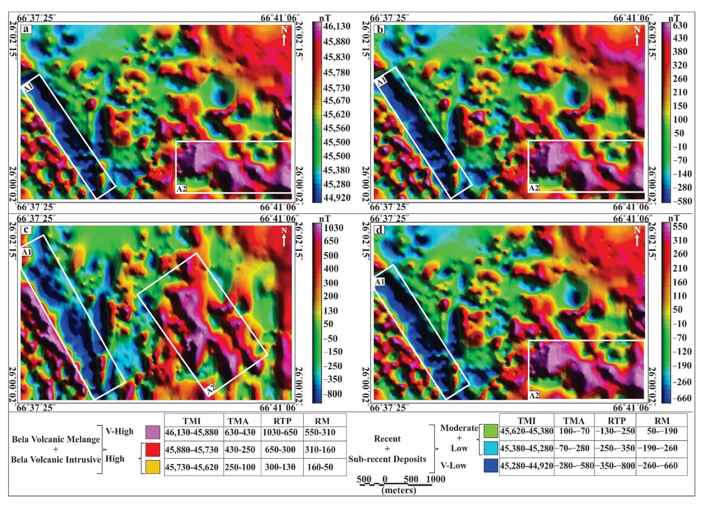
• In the SE part of the study area, a positive high-magnetic anomaly (A2) is observed, which shows the presence of an ultramafic sequence of BOC. Rocks that show paramagnetic response indicate manganese-ore deposits with a residual magnetic signature of 310–550 nT. In contrast, a negative magnetic anomaly (A1) is observed in the western part of the study area that ranges between −190 nT to 50 nT. This NW–SE trending low-anomalous zone is interpreted by RTP, TMI, HG, and RM as a shear zone covered by alluvium.
• Resistivity and IP surveys are conducted along the low-magnetic zone (A1) for any sulfide mineralization, and the resistivity values fluctuate between 10 Ωm to 80 Ωm, which shows the presence of clay minerals covered by alluvium to a depth of 50 m. The resistivity values gradually increase and reach a peak value of 4000 Ωm, confirming the presence of the ultramafic sequence at greater depths. The sulfide deposits are supposed to produce a low-resistivity signal with high chargeability; however, the IP values fluctuate between 0.7 mV/V and 4 mV/V. This low-anomalous zone contains clay minerals, confirming no sulfide mineralization, and are strongly supported by VES and magnetic data, so are interpreted as a shear zone.
• The high-magnetic-anomalous zone (A2) is interpreted as Mn mineralization supported by a high-magnetic value and a high IP signature of 3.5 mV/V to 15.1 mV/V.
• The geochemical analysis along the high-magnetic zone verifies a very good deposit of Mn minerals, with a percentage composition of 36.5% for rock samples and 48,400 ppm, along with stream analysis.
• The statistical analysis demarcates the magnetic anomalous base value of 46,181 nT to 46,628 nT of total intensity and 783 nT to 1183 nT, which is used for the determination of Mn mineralization elsewhere along the BOC.
• The horizontal-filter map shows a series of concealed faults, by applying a horizontal linear filter covered by alluvium with major orientations in the NW–SE and N–S directions, indicating that the BOC has thrust upwards in the NW direction over Late Tertiary sediments associated with melange, represented by chaotic-mineral assemblage that is revealed by the geomagnetic section (A-B).
• Structurally, the study area is highly disturbed and a series of faults are formed, showing the tectonic forces in the E–W direction and the presence of horst and graben structures in the form of the shear zone, developed under the extensional regime and inferred from the geomagnetic section (A-B).
• The geomagnetic maps reveal that the Bela melange of the moderate magnetic signature accommodating Mn mineralization along the anticlinal zone corresponds to high-magnetic imprints other than Bela melange. While the Bela volcanic intrusive corresponds to a low-magnetic value compared to the mélange, which is characterized by alteration of the volcanic intrusive.
• The outcomes of this study could be fruitful for prioritizing zones of the prospect area to delineate lineaments and target zones that are of vital interest to the minerals sector of Pakistan.

References

1. Yao, J.; Cawood, P.A.; Zhao, G.; Han, Y.; Xia, X.; Liu, Q.; Wang, P. Mariana-type ophiolites constrain the establishment of modern plate tectonic regime during Gondwana assembly. Nat. Commun. 2021, 12, 4189. [Google Scholar] [CrossRef] [PubMed]
2. Sotiriou, P.; Polat, A. Comparisons between Tethyan Anorthosite-Bearing Ophiolites and Archean Anorthosite-Bearing Layered Intrusions: Implications for Archean Geodynamic Processes. Tectonics 2020, 39, e2020TC006096. [Google Scholar] [CrossRef]
3. Wang, G.; Zhang, P. A New Understanding on the Emplacement of Ophiolitic Mélanges and Its Tectonic Significance: Insights from the Structural Analysis of the Remnant Oceanic Basin-Type Ophiolitic Mélanges. Acta Geol. Sin. Engl. Ed. 2020, 94, 60–62. [Google Scholar] [CrossRef]
4. Zhang, P.F.; Zhou, M.F.; Yumul, G.P., Jr.; Wang, C.Y. Geodynamic setting of high-Cr chromite mineralization in nascent subduction zones: Li isotopic and REE constraints from the Zambales ophiolite, Philippines. Lithos 2021, 384, 105975. [Google Scholar] [CrossRef]
5. Karimzadeh, H.; Rahgoshay, M.; Monsef, I. Mineralogy, Geochemistry, and Petrogenesis of Mantle Peridotites of Nehbandan Ophiolitic Complex, East of Iran. J. Econ. Geol. 2020, 12, 157–176. [Google Scholar]
6. Kiseleva, O.N.; Airiyants, E.V.; Belyanin, D.K.; Zhmodik, S.M. Podiform chromitites and PGE mineralization in the Ulan-Sar’dag ophiolite (East Sayan, Russia). Minerals 2020, 10, 141. [Google Scholar] [CrossRef] [Green Version]
7. Yang, J.; Wu, W.; Lian, D.; Rui, H. Peridotites, chromitites, and diamonds in ophiolites. Nat. Rev. Earth Environ. 2021, 2, 198–212. [Google Scholar] [CrossRef]
8. Ullah, Z.; Shah, M.T.; Siddiqui, R.H.; Lian, D.-Y.; Khan, A.A. Petrochemistry of High-Cr and High-Al chromitites occurrences of Dargai Complex along Indus Suture Zone, Northern Pakistan. Episodes 2020, 43, 689–709. [Google Scholar] [CrossRef] [Green Version]
9. Zaccarini, F.; Ifandi, E.; Tsikouras, B.; Grammatikopolous, T.; Garuti, G.; Mauro, D.; Bindi, L.; Stanley, C. Occurrence of new phosphides and sulfides of Ni, Co, V, and Mo from chromitite of the Othrys ophiolite complex (Central Greece). Per. Ital. Mineral 2019, 88, 29–43. [Google Scholar] [CrossRef]
10. Uysal, I.; Akmaz, R.M.; Saka, S.; Kapsiotis, A. Coexistence of compositionally heterogeneous chromitites in the Antalya–Isparta ophiolitic suite, SW Turkey: A record of sequential magmatic processes in the sub-arc lithospheric mantle. Lithos 2016, 248, 160–174. [Google Scholar] [CrossRef]
11. Bashir, E.; Naseem, S.; Kaleem, M.; Khan, Y.; Hamza, S. Study of Serpentinized Ultramafic Rocks of Bela Ophiolite, Balochistan, Pakistan. J. Geogr. Geol. 2012, 4, 79. [Google Scholar] [CrossRef]
12. Zaigham, N.A.; Mallick, K.A. Bela ophiolite zone of southern Pakistan: Tectonic setting and associated mineral deposits. GSA Bull. 2000, 112, 478–489. [Google Scholar] [CrossRef]
13. Sarwar, G. Tectonic setting of the Bela Ophiolites, southern Pakistan. Tectonophysics 1992, 207, 359–381. [Google Scholar] [CrossRef]
14. Xiong, Y.; Khan, S.D.; Mahmood, K.; Sisson, V.B. Lithological mapping of Bela ophiolite with remote-sensing data. Int. J. Remote Sens. 2011, 32, 4641–4658. [Google Scholar] [CrossRef]
15. Gnos, E.; Khan, A.S.; Mahmood, K.; Villa, I.M. Bela oceanic lithosphere assemblage and its relation to the Réunion hotspot. Terra Nova 1998, 10, 90–95. [Google Scholar] [CrossRef]
16. Naseem, S.; Sheikh, S. Lithogeochemical Prospecting Through Stream Sediments in Bela Ophiolite of Lasbela Area. J. King Abdulaziz Univ. Sci. 1994, 7, 125–142. [Google Scholar] [CrossRef]
17. Ahsan, S.N.; Quraishi, I.H. Mineral-Rock Resources of Lasbela and Khuzdar Districts, Balochistan, Pakistan. J. Himal. Earth Sci. 1997, 30, 41–51. [Google Scholar]
18. Ali, S.I. A study of manganese ore deposits, Las Bela, West Pakistan. Acta Miner petrogr Szeged. 1971, 1, 141–148. [Google Scholar]
19. Naseem, S.; Sheikh, S.A.; Qadeeruddin, M. Biogeochemical study of Tamarix aphylla from Lasbela area and its application in prospecting of ore deposits. Chin. J. Geochem. 1995, 14, 303–312. [Google Scholar] [CrossRef]
20. Narejo, A.A.; Shar, A.M.; Fatima, N.; Sohail, K. Geochemistry and origin of Mn deposits in the Bela ophiolite complex, Balochistan, Pakistan. J. Pet. Explor. Prod. Technol. 2019, 9, 2543–2554. [Google Scholar] [CrossRef] [Green Version]
21. Shah, S.H.A. The ophiolite belts and suture traces in Pakistan. J. Himal. Earth Sci. 1984, 17, 113–117. [Google Scholar]
22. Canada, P.I.O.M. Aeromagnetic Interpretation of Khuzdar Bela Region Balochistan Pakistan; Geological Survey of Pakistan: Ministry of Petroleum and Natural Resources & Govt of Canada, Photosur Inc: Montreal, QC, Canada, 1981. [Google Scholar]
23. Abedi, M.; Gholami, A.; Norouzi, G.-H. A stable downward continuation of airborne magnetic data: A case study for mineral prospectivity mapping in Central Iran. Comput. Geosci. 2013, 52, 269–280. [Google Scholar] [CrossRef]
24. Kang, G.; Gao, G.; Bai, C.; Shao, D.; Feng, L. Characteristics of the crustal magnetic anomaly and regional tectonics in the Qinghai-Tibet Plateau and the adjacent areas. Sci. China Earth Sci. 2011, 55, 1028–1036. [Google Scholar] [CrossRef]
25. Liang, R.; Pei, Y.; Zheng, Y.; Wei, J.; Liu, Y. Gravity and magnetic field and tectonic structure character in the southern Yellow Sea. Chin. Sci. Bull. 2003, 48, 64–73. [Google Scholar] [CrossRef]
26. Rybakov, M.; Goldshmidt, V.; Hall, J.; Ben-Avraham, Z.; Lazar, M. New insights into the sources of magnetic anomalies in the Levant. Russ. Geol. Geophys. 2011, 52, 377–397. [Google Scholar] [CrossRef]
27. Quesnel, Y.; Weckmann, U.; Ritter, O.; Stankiewicz, J.; Lesur, V.; Mandea, M.; Langlais, B.; Sotin, C.; Galdéano, A. Simple models for the Beattie Magnetic Anomaly in South Africa. Tectonophysics 2009, 478, 111–118. [Google Scholar] [CrossRef] [Green Version]
28. Yatini, Y.; Zakaria, M.F.; Suyanto, I. Identification of Gold Mineralization Zones Using Magnetic Data at Gunung Gupit Area, Magelang, Central Java. In RSF Conference Series: Engineering and Technology; Research Synergy Foundation Press: Bandung, Indonesia, 2021; Volume 1, pp. 305–312. [Google Scholar] [CrossRef]
29. Ewusi, A.; Adatsi, E.; Seidu, J. Integrated geophysical study to delineate mineralized zones in southwest Ashanti Belt of Ghana. J. Geosci. Environ. Prot. 2018, 6, 77. [Google Scholar]
30. Hasan, M.; Shang, Y.; Jin, W. Delineation of weathered/fracture zones for aquifer potential using an integrated geophysical approach: A case study from South China. J. Appl. Geophys. 2018, 157, 47–60. [Google Scholar] [CrossRef]
31. Araffa, S.A.S.; Santos, F.A.M.; Arafa-Hamed, T. Delineating active faults by using integrated geophysical data at northeastern part of Cairo, Egypt. NRIAG J. Astron. Geophys. 2012, 1, 33–44. [Google Scholar] [CrossRef] [Green Version]
32. Milsom, J. Field Geophysics; John Wiley and Sons Ltd: Chichester, UK, 2007. [Google Scholar]
33. Tchokpon, K.G.; Kaki, C.; Kourouma, M.; Yalo, N. Detection of gold-bearing quartz veins in the meta-sedimentary formation in the North-Eastern Guinea using remote sensing and geophysical exploration. J. Afr. Earth Sci. 2020, 168, 103869. [Google Scholar] [CrossRef]
34. Naskar, D.C.; Kulkarni, A.V.; Lakshmana, M. Geophysical investigation for base metal mineralization in Karoi-Rajpura area, Bhilwara district, Rajasthan. J. Ind. Geophys. Union 2018, 22, 379–388. [Google Scholar]
35. Riddihough, R.P. Diurnal Corrections to Magnetic Surveys-an Assessment of Errors. Geophys. Prospect. 1971, 19, 551–567. [Google Scholar] [CrossRef]
36. Bloxham, J.; Gubbins, D.; Jackson, A. Geomagnetic secular variation. Philosophical Transactions of the Royal Society of London. Ser. A Math. Phys. Sci. 1989, 329, 415–502. [Google Scholar]
37. Mahboubian, F.; Sardari, H.; Sadeghi, S.; Sarreshtedari, F. Design and Implementation of a Low Noise Earth Field Proton Precession Magnetometer. In Proceedings of the 2019 27th Iranian Conference on Electrical Engineering (ICEE), Yazd, Iran, 30 April–2 May 2019; pp. 345–347. [Google Scholar]
38. Fedi, M.; Florio, G.; Rapolla, A. A method to estimate the total magnetization direction from a distortion analysis of magnetic anomalies1. Geophys. Prospect. 1994, 42, 261–274. [Google Scholar] [CrossRef]
39. Foss, C. Magnetic Data Enhancements and Depth Estimation. In Encyclopedia of Solid Earth Geophysics; Gupta, H.K., Ed.; Springer International Publishing: Cham, Switzerland, 2020. [Google Scholar] [CrossRef]
40. Azad, M. Application of Upward Continuation Filter in the interpretation of Magnetic Data with the determination of Optimum Height Continuation, Mansoorabad Area of Yazd, Iran. J. Earth Space Phys. 2015, 41, 229–238. [Google Scholar]
41. Hinze, W.J.; Von Frese, R.R.; Von Frese, R.; Saad, A.H. Gravity and Magnetic Exploration: Principles, Practices, and Applications; Cambridge University Press: Cambridge, UK, 2013. [Google Scholar]
42. Cooper, G. The downward continuation of aeromagnetic data from magnetic source ensembles. Near Surf. Geophys. 2019, 17, 101–107. [Google Scholar] [CrossRef]
43. Cooper, G.R.J.; Cowan, D.R. Filtering using variable order vertical derivatives. Comput. Geosci. 2004, 30, 455–459. [Google Scholar] [CrossRef]
44. Stanley, J.M. Simplified Magnetic Interpretation of the Geologic Contact and Thin Dike. Geophysics 1977, 42, 1236–1240. [Google Scholar] [CrossRef]
45. El All, E.A.; Khalil, A.; Rabeh, T.; Osman, S. Geophysical contribution to evaluate the subsurface structural setting using magnetic and geothermal data in El-Bahariya Oasis, Western Desert, Egypt. NRIAG J. Astron. Geophys. 2015, 4, 236–248. [Google Scholar] [CrossRef] [Green Version]
46. Reid, A.B.; Allsop, J.M.; Granser, H.; Millett, A.J.; Somerton, I.W. Magnetic interpretation in three dimensions using Euler deconvolution. Geophysics 1990, 55, 80–91. [Google Scholar] [CrossRef] [Green Version]
47. Thompson, D.T. EULDPH: A new technique for making computer-assisted depth estimates from magnetic data. Geophysics 1982, 47, 31–37. [Google Scholar] [CrossRef]
48. Stavrev, P.; Reid, A. Degrees of homogeneity of potential fields and structural indices of Euler deconvolution. Geophysics 2007, 72, L1–L12. [Google Scholar] [CrossRef]
49. Stavrev, P.; Reid, A. Euler deconvolution of gravity anomalies from thick contact/fault structures with extended negative structural index. Geophysics 2010, 75, I51–I58. [Google Scholar] [CrossRef]
50. El-Makky, A.M.; Sediek, K.N. Stream Sediments Geochemical Exploration in the Northwestern Part of Wadi Allaqi Area, South Eastern Desert, Egypt. Nonrenewable Resour. 2012, 21, 95–115. [Google Scholar] [CrossRef]
51. Ravisankar, R.; Tholkappian, M.; Chandrasekaran, A.; Eswaran, P.; El-Taher, A. Effects of physicochemical properties on heavy metal, magnetic susceptibility and natural radionuclides with statistical approach in the Chennai coastal sediment of east coast of Tamilnadu, India. Appl. Water Sci. 2019, 9, 151. [Google Scholar] [CrossRef] [Green Version]
52. Soupios, P.M.; Kouli, M.; Vallianatos, F.; Vafidis, A.; Stavroulakis, G. Estimation of aquifer hydraulic parameters from surficial geophysical methods: A case study of Keritis Basin in Chania (Crete–Greece). J. Hydrol. 2007, 338, 122–131. [Google Scholar] [CrossRef]
53. Bobachev, C. IPI2Win: A Windows Software for an Automatic Interpretation of Resistivity Sounding Data; Moscow State University: Moscow, Russia, 2002; Volume 320. [Google Scholar]
54. Daneshvar Saein, L.; Rasa, I.; Rashidnejad Omran, N.; Moarefvand, P.; Afzal, P. Application of the concentration-volume fractal method in induced polarization and resistivity data interpretation for Cu-Mo porphyry deposits exploration, case study: Nowchun Cu-Mo deposit, SE Iran. Nonlinear Processes Geophys. 2012, 19, 431–438. [Google Scholar] [CrossRef]
55. Hördt, A.; Hanstein, T.; Hönig, M.; Neubauer, F.M. Efficient spectral IP-modelling in the time domain. J. Appl. Geophys. 2006, 59, 152–161. [Google Scholar] [CrossRef]
56. Seigel, H.O.; Vanhala, H.; Sheard, S.N. Some case histories of source discrimination using time-domain spectral IP. Geophysics 1997, 62, 1394–1408. [Google Scholar] [CrossRef]
57. Vieira, L.B.; Moreira, C.A.; Côrtes, A.R.P.; Luvizotto, G.L. Geophysical modeling of the manganese deposit for Induced Polarization method in Itapira (Brazil). Geofísica Int. 2016, 55, 107–117. [Google Scholar] [CrossRef]
58. Ramazi, H.; Mostafaie, K. Application of integrated geoelectrical methods in Marand (Iran) manganese deposit exploration. Arab. J. Geosci. 2012, 6, 2961–2970. [Google Scholar] [CrossRef]
59. Moreira, C.A.; Borges, M.R.; Vieira, G.M.L.; Filho, W.M.; Montanheiro, M.A.F. Geological and geophysical data integration for delimitation of mineralized areas in a supergene manganese deposits. Geofísica Int. 2014, 53, 199–210. [Google Scholar] [CrossRef]
60. Taufan, Y.A.; Denis, M.; Nur, A.A.; Syafri, I. Manganese Prospect Identification Using Magnetic and Induced Polarization Methods. Bull. Sci. Contrib. Geol. 2018, 16, 215–220. [Google Scholar]
61. Kwan, K.; Müller, D. Mount Milligan alkalic porphyry Au--Cu deposit, British Columbia, Canada, and its AEM and AIP signatures: Implications for mineral exploration in covered terrains. J. Appl. Geophys. 2020, 180, 104131. [Google Scholar] [CrossRef]
62. Dusabemariya, C.; Qian, W.; Bagaragaza, R.; Faruwa, A.R.; Ali, M. Some Experiences of Resistivity and Induced Polarization Methods on the Exploration of Sulfide: A Review. J. Geosci. Environ. Prot. 2020, 8, 68–92. [Google Scholar] [CrossRef]
63. Kumar, P.; Tiwari, P.; Singh, A.; Biswas, A.; Acharya, T. Electrical Resistivity and Induced Polarization signatures to delineate the near-surface aquifers contaminated with seawater invasion in Digha, West-Bengal, India. CATENA 2021, 207, 105596. [Google Scholar] [CrossRef]
Figure 1. (a) Ophiolitic map of Pakistan showing different Ophiolitic occurrences in the study area, (b) geological and base map showing locations of magnetic observation, VES, and location of rocks and stream-sediment samples, (c) geological cross section along profile A-B, modified after [13].
Minerals 12 00825 g001
Figure 2. (a) Total Magnetic Intensity (TMI), (b) Total Magnetic Anomaly (TMA), (c) Reduction to Pole (RTP), (d) Residual Magnetic (RM).
Minerals 12 00825 g002
Figure 3. (a) Upward Continuation (UC) of RTP by 100m, (b) Downward Continuation (DC) of RTP by 100 m, (c) Vertical Derivative (VD), (d) Horizontal Gradient (HG).
Minerals 12 00825 g003
Figure 4. (a) Geomagnetic map of the study area showing overall magnetic signatures, (b) magnetic cross section along A-B showing magnetic signature at depth, (c) magnetic profile along A-B showing changing magnetic anomaly with distance and depth.
Minerals 12 00825 g004
Figure 5. (a) Euler convolution map of the study area showing depth range, (b) Euler depth map of high-anomalous zone A2, (c) Euler depth map of low-anomalous zone A1.
Minerals 12 00825 g005
Figure 6. Statistical analysis of TMA and TMI each show three clusters CI, CII, and CIII, and CAI, CAII, and CAIII, respectively.
Minerals 12 00825 g006
Figure 7. Geoelectrical Section of low- (A1) and high-magnetic- (A2) anomalous zones arranged along VES-01, VES-02, and VES-03 representing A1 zone (ac) and A2 zone (df).
Minerals 12 00825 g007
Figure 8. Pseudo section and true resistivity section along with low-magnetic-anomalous zone A1 (a,b) and high-magnetic-anomalous zone A2 (c,d).
Minerals 12 00825 g008