
Comparison of Geometric Properties of Regular and Irregular Mineral Grains by Dynamic Image Analysis (2D) and Optoelectronic Analysis (3D) Methods


Abstract
:1. Introduction
2. Materials and Methods
2.1. Purpose and Scope of the Research
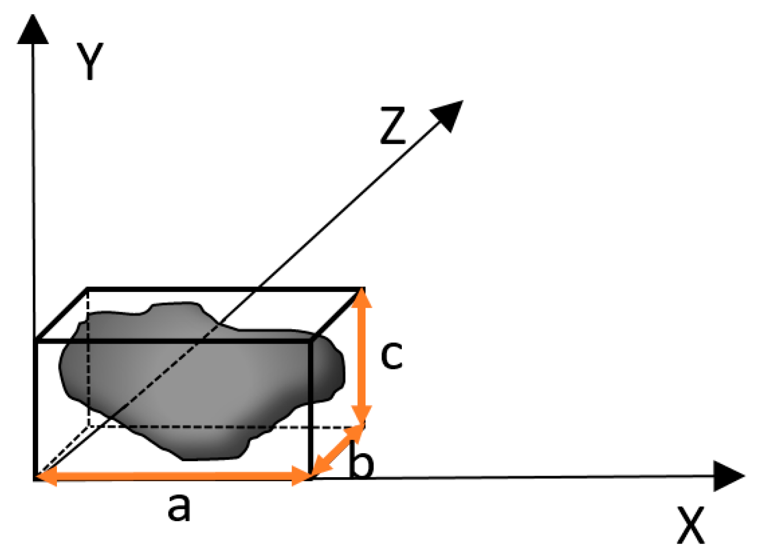
2.2. Shape Descriptors
2.3. Measurement Methods
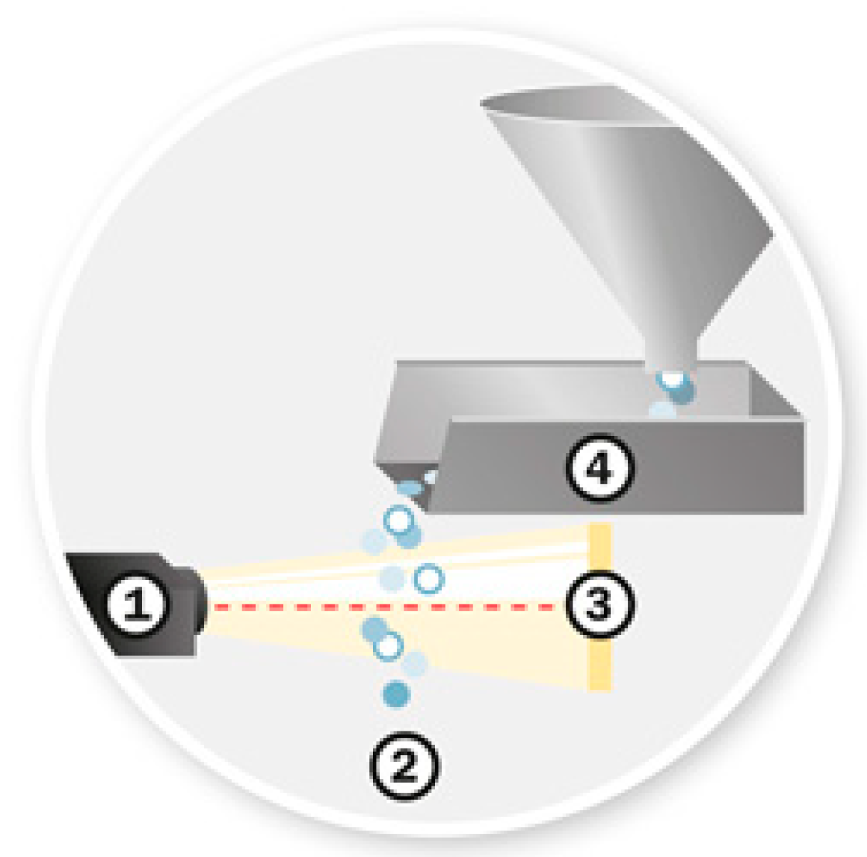
2.3.1. 2D Imaging
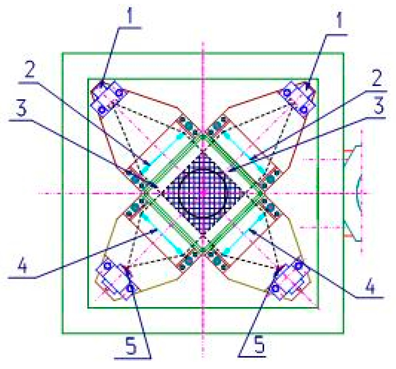
2.3.2. 3D Imaging
3. Discussion
3.1. Assessment of Grain Size Distribution
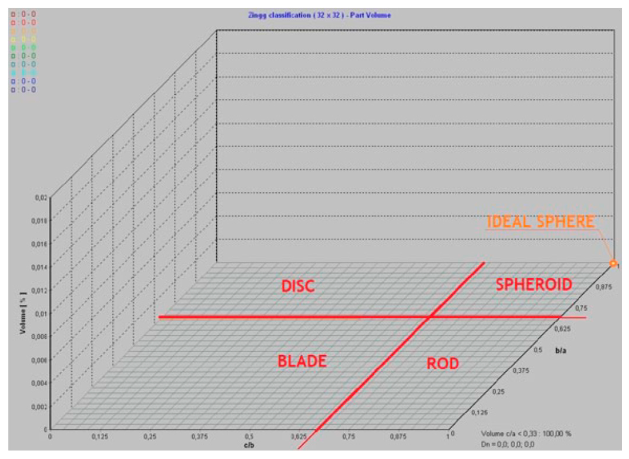
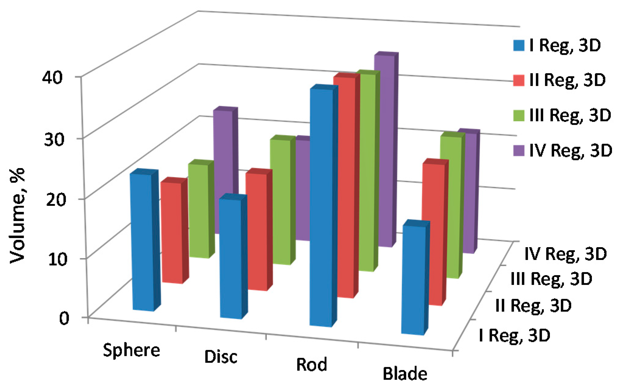
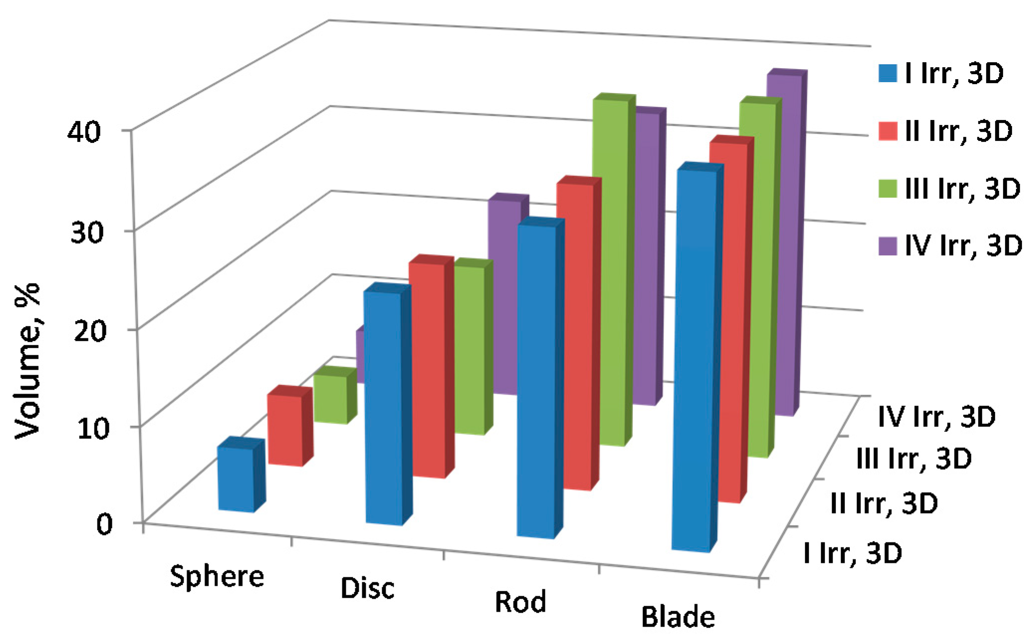
3.2. Evaluation of Grain Shapes
4. Conclusions
Author Contributions
Funding
Data Availability Statement
Conflicts of Interest
References
- EN 933-3:2012; Tests for Geometrical Properties of Aggregates-Part 3: Determination of Particle Shape-Flakiness Index. CEN European Committee for Standarization: Brussels, Belgium, 2012.
- EN 933-4:2008; Tests for Geometrical Properties of Aggregates-Part 4: Determination of Particle Shape-Shape Index. European Committee for Standarization: Brussels, Belgium, 2008.
- Zieliński, Z. Korelacja Parametrów Technologicznych Mechanicznego Kruszenia i Przesiewania Materiałów Skalnych Stosowanych w Budownictwie Drogowym; Wydawnictwo Uczelniane Politechniki Szczecińskiej: Szczecin, Poland, 1983; p. 228. [Google Scholar]
- Tumidajski, T.; Naziemiec, Z. Wpływ warunków procesu kruszenia na kształt ziaren kruszyw mineralnych. In Proceedings of the IV Konferencja Kruszywa Mineralne Surowce-Rynek-Technologie-Jakość, Szklarska Poręba, Poland, 14–16 April 2004; Wydawnictwo Politechnika Wrocławska: Wrocław, Poland, 2004. [Google Scholar]
- Naziemiec, Z.; Gawenda, T. Ocena efektów rozdrabniania surowców mineralnych w różnych urządzeniach kruszących. In Proceedings of the VI Konferencja, Kruszywa Mineralne–Surowce–Rynek–Technologie–Jakoś, Szklarska Poręba, Poland, 26–28 April 2006; OWPW: Wrocław, Poland, 2006; pp. 83–94. [Google Scholar]
- Neville, A.M. Właściwości Betonu, 4th ed.; Polski Cement: Kraków, Poland, 2000. [Google Scholar]
- Malewski, J. Kształt ziaren w produktach kruszenia. Kruszywa 2014, 3, 52–55. [Google Scholar]
- Gawenda, T. Innowacyjne technologie produkcji kruszyw o ziarnach foremnych. Prace Naukowe Instytutu Górnictwa Politechniki Wrocławskiej. Górnictwo Geol. 2015, 22, 45–59. [Google Scholar]
- Gawenda, T. Zasady Doboru Kruszarek Oraz Układów Technologicznych w Produkcji Kruszyw Łamanych; AGH University of Science and Technology Press: Cracow, Poland, 2015; pp. 1–232. [Google Scholar]
- Mitchell, J.K.; Soga, K. Fundamentals of Soil Behavior, 3rd ed.; Wiley: New York, NY, USA, 2005; ISBN 978-0-471-46302-3. [Google Scholar]
- Cho, G.-C.; Dodds, J.; Santamarina, J.C. Particle Shape Effects on Packing Density, Stiffness, and Strength: Natural and Crushed Sands. J. Geotech. Geoenviron. Eng. 2006, 132, 591–602. [Google Scholar] [CrossRef] [Green Version]
- Pestana, J.M.; Whittle, A.J. Compression model for cohesionless soils. Géotechnique 1995, 45, 611–631. [Google Scholar] [CrossRef]
- Rousé, P.C.; Fannin, R.J.; Shuttle, D.A. Influence of roundness on the void ratio and strength of uniform sand. Géotechnique 2008, 58, 227–231. [Google Scholar] [CrossRef]
- Bessa, I.S.; Branco, V.T.F.C.; Soares, J.B.; Neto, J.A.N. Aggregate Shape Properties and Their Influence on the Behavior of Hot-Mix Asphalt. J. Mater. Civ. Eng. 2015, 27, 4014212. [Google Scholar] [CrossRef]
- Connolly, B.J.; Loth, E.; Smith, C.F. Shape and drag of irregular angular particles and test dust. Powder Technol. 2020, 363, 275–285. [Google Scholar] [CrossRef]
- KKnoll, M.; Gerhardter, H.; Prieler, R.; Mühlböck, M.; Tomazic, P.; Hochenauer, C. Particle classification and drag coefficients of irregularly-shaped combustion residues with various size and shape. Powder Technol. 2019, 345, 405–414. [Google Scholar] [CrossRef]
- Krumbein, W.C. Settling-velocity and flume-behavior of non-spherical particles. Trans. Am. Geophys. Union 1942, 23, 621–633. [Google Scholar] [CrossRef]
- Jonasz, M. Nonsphericity of suspended marine particles and its influence on light scattering1. Limnol. Oceanogr. 1987, 32, 1059–1065. [Google Scholar] [CrossRef]
- Krawczykowski, D. Application of a vision systems for assessment of particle size and shape for mineral crushing products. IOP Conf. Ser. Mater. Sci. Eng. 2018, 427, 012013. [Google Scholar] [CrossRef] [Green Version]
- Beuselinck, L.; Govers, G.; Poesen, J.; Degraer, G.; Froyen, L. Grain-size analysis by laser diffractometry: Comparison with the sieve-pipette method. Catena 1998, 32, 193–208. [Google Scholar] [CrossRef]
- Li, M.; Wilkinson, D.; Patchigolla, K. Comparison of Particle Size Distributions Measured Using Different Techniques. Part. Sci. Technol. 2005, 23, 265–284. [Google Scholar] [CrossRef]
- Xu, R.; Di Guida, O.A. Comparison of sizing small particles using different technologies. Powder Technol. 2003, 132, 145–153. [Google Scholar] [CrossRef]
- Shang, Y.; Kaakinen, A.; Beets, C.J.; Prins, M.A. Aeolian silt transport processes as fingerprinted by dynamic image analysis of the grain size and shape characteristics of Chinese loess and Red Clay deposits. Sediment. Geol. 2018, 375, 36–48. [Google Scholar] [CrossRef]
- Sneed, E.D.; Folk, R.L. Pebbles in the Lower Colorado River, Texas a Study in Particle Morphogenesis. J. Geol. 1958, 66, 114–150. [Google Scholar] [CrossRef]
- Krumbein, W.C. Measurement and Geological Significance of Shape and Roundness of Sedimentary Particles. J. Sediment. Res. 1941, 11, 64–72. [Google Scholar] [CrossRef]
- Wentworth, C.K. The Shapes of Beach Pebbles. US Geological Survey Professional Paper; US Government Printing Office: Washington, DC, USA, 1922; Volume 131, pp. 75–83.
- Zingg, T. Beitrag zur Schotteranalyse. Schweizer Miner. Petrog. Mitt. 1935, 15, 39–140. [Google Scholar]
- Allen, T. Powder Sampling and Particle Size Determination, 1st ed.; Elsevier Science: London, UK, 2003; ISBN 9780080539324. [Google Scholar]
- Rodriguez, J.; Edeskär, T.; Knutsson, S. Particle shape quantities and measurement techniques: A review. Electron. J. Geotech. Eng. 2013, 18, 169–198. [Google Scholar]
- Krawczykowski, D. Unification of the Results of Granulometric Analyzes of Finegrained Mineral Powders; Dissertations and Monographs 347; AGH University of Science and Technology: Krakow, Poland, 2019. [Google Scholar]
- Illenberger, W.K. Pebble Shape (and Size!). J. Sediment. Res. 1991, 61, 756–767. [Google Scholar]
- Bott, S.J.; Pye, K. Particle shape: A review and new methods of characterization and classification. Sedimentology 2008, 55, 31–63. [Google Scholar]
- Freund, Y.; Schapire, R.E. A Decision-Theoretic Generalization of On-Line Learning and an Application to Boosting. J. Comput. Syst. Sci. 1997, 55, 119–139. [Google Scholar] [CrossRef] [Green Version]
- Zheng, J.; Hryciw, R.D. Identification and Characterization of Particle Shapes from Images of Sand Assemblies Using Pattern Recognition. J. Comput. Civ. Eng. 2018, 32, 04018016. [Google Scholar] [CrossRef]
- Liang, Z.; Nie, Z.; An, A.; Gong, J.; Wang, X. A particle shape extraction and evaluation method using a deep convolutional neural network and digital image processing. Powder Technol. 2019, 353, 156–170. [Google Scholar] [CrossRef]
- Riley, C.M.; Rose, W.I.; Bluth, G.J.S. Quantitative shape measurements of distal volcanic ash. J. Geophys. Res. Earth Surf. 2003, 108, 2504. [Google Scholar] [CrossRef] [Green Version]
- Taylor, M.; Garboczi, E.; Erdogan, S.; Fowler, D. Some properties of irregular 3-D particles. Powder Technol. 2006, 162, 1–15. [Google Scholar] [CrossRef]
- Alfano, F.; Bonadonna, C.; Delmelle, P.; Costantini, L. Insights on tephra settling velocity from morphological observations. J. Volcanol. Geotherm. Res. 2011, 208, 86–98. [Google Scholar] [CrossRef]
- Lin, C.; Miller, J. 3D characterization and analysis of particle shape using X-ray microtomography (XMT). Powder Technol. 2005, 154, 61–69. [Google Scholar] [CrossRef]
- Ersoy, O.; Şen, E.; Aydar, E.; Tatar, İ.; Çelik, H.H. Surface area and volumemeasurements of volcanic ash particles using micro-computed tomography (micro-CT): A comparison with scanning electron microscope (SEM) stereoscopic imaging and geometric considerations. J. Volcanol. Geotherm. Res. 2010, 196, 281–286. [Google Scholar] [CrossRef]
- Mills, O.P.; Rose, W.I. Shape and surface area measurements using scanning elektron microscope stereo-pair images of volcanic ash particles. Geosphere 2010, 6, 805–811. [Google Scholar] [CrossRef] [Green Version]
- Asahina, D.; Taylor, M. Geometry of irregular particles: Direct surface measurements by 3-D laser scanner. Powder Technol. 2011, 213, 70–78. [Google Scholar] [CrossRef]
- Garboczi, E.; Liu, X.; Taylor, M. The 3-D shape of blasted and crushed rocks: From 20μm to 38mm. Powder Technol. 2012, 229, 84–89. [Google Scholar] [CrossRef]
- Ersoy, O. Surface area and volume measurements of volcanic ash particles by SEM stereoscopic imaging. J. Volcanol. Geotherm. Res. 2010, 190, 290–296. [Google Scholar] [CrossRef]
- Bullard, J.W.; Garboczi, E.J. Defining shape measures for 3D star-shaped particles: Sphericity, roundness, and dimensions. Powder Technol. 2013, 249, 241–252. [Google Scholar] [CrossRef]
- White, D.J. PSD measurement using the single particle optical sizing (SPOS) method. Geotechnique 2003, 53, 317–326. [Google Scholar] [CrossRef]
- Altuhafi, F.; O’Sullivan, C.; Cavarretta, I. Analysis of an Image-Based Method to Quantify the Size and Shape of Sand Particles. J. Geotech. Geoenviron. Eng. 2013, 139, 1290–1307. [Google Scholar] [CrossRef]
- Bowman, E.; Soga, K.; Drummond, W. Particle shape characterization using Fourier descriptor analysis. Geotechnique 2001, 51, 545–554. [Google Scholar] [CrossRef]
- Sukumaran, B.; Ashmawy, A. Quantitative characterization of discrete particles. Geotechnique 2001, 51, 619–627. [Google Scholar] [CrossRef]
- Garboczi, E.; Hrabe, N. Particle shape and size analysis for metal powders used for additive manufacturing: Technique description and application to two gas-atomized and plasma-atomized Ti64 powders. Addit. Manuf. 2020, 31, 100965. [Google Scholar] [CrossRef]
- Bay, B.K.; Smith, T.S.; Fyhrie, D.P.; Saad, M. Digital volume correlation: Three-dimensional strain mapping using X-ray tomography. Exp. Mech. 1999, 39, 217–226. [Google Scholar] [CrossRef]
- Gawenda, T.; Saramak, D.; Nad, A.; Surowiak, A.; Krawczykowska, A.; Foszcz, D. Badania procesu uszlachetniania kruszyw w innowacyjnym układzie technologicznym. In Proceedings of the XIX Konferencja Kruszywa Mineralne Surowce-Rynek-Technologie-Jakość, Kudowa Zdrój, Poland, 24–26 April 2019. [Google Scholar]
- Gawenda, T.; Krawczykowski, D.; Krawczykowska, A.; Saramak, A.; Nad, A. Application of Dynamic Analysis Methods into Assessment of Geometric Properties of Chalcedonite Aggregates Obtained by Means of Gravitational Upgrading Operations. Minerals 2020, 10, 180. [Google Scholar] [CrossRef] [Green Version]
- Bagheri, G.H.; Bonadonna, C.; Manzella, I.; Vonlanthen, P. On the characterization of size and shape of irregular particles. Powder Technol. 2015, 270, 141–153. [Google Scholar] [CrossRef]
- Krumbein, W.C.; Sloss, L.L. Stratigraphy and Sedimentation; W.H. Freeman and Company: San Francisco, CA, USA, 1951. [Google Scholar]
- Mora, C.F.; Kwan, A.K.H. Sphericity, shape factor, and convexity measurement of coarse aggregate for concrete using digital image processing. Cem. Concr. Res. 2000, 30, 351–358. [Google Scholar] [CrossRef]
- Riley, N.A. Projection sphericity. J. Sediment. Res. 1941, 11, 94–95. [Google Scholar] [CrossRef]
- Wadell, H. Sphericity and Roundness of Rock Particles. J. Geol. 1933, 41, 310–331. [Google Scholar] [CrossRef]
- Santamarina, J.C.; Cho, G.C. Soil behaviour: The role of particle shape. In Advances in Geotechnical Engineering: The Skempton Conference; Thomas Telford Publishing: London, UK, 2004; pp. 604–617. [Google Scholar]
- Kuo, C.-Y.; Freeman, R.B. Imaging Indices for Quantification of Shape, Angularity, and Surface Texture of Aggregates. Transp. Res. Rec. J. Transp. Res. Board 2000, 1721, 57–65. [Google Scholar] [CrossRef]
- Wadell, H. Volume, Shape, and Roundness of Rock Particles. J. Geol. 1932, 40, 443–451. [Google Scholar] [CrossRef]
- Mandelbrot, B. How Long Is the Coast of Britain? Statistical Self-Similarity and Fractional Dimension. Science 1967, 156, 636–638. [Google Scholar] [CrossRef] [Green Version]
- Cox, E.P. A method of assigning numerical and percentage values to the degree of roundness of sand grains. J. Paleontol. 1927, 1, 179–183. [Google Scholar]
- Su, D.; Yan, W.M. 3D characterization of general-shape sand particles using microfocus X-ray computed tomography and spherical harmonic functions, and particle regeneration using multivariate random vector. Powder Technol. 2018, 323, 8–23. [Google Scholar] [CrossRef]
- Yan, P.; Zhang, J.; Fang, Q.; Zhang, Y.; Fan, J. 3D numerical modelling of solid particles with randomness in shape considering convexity and concavity. Powder Technol. 2016, 301, 131–140. [Google Scholar] [CrossRef]
- Zhao, B.; Wang, J. 3D quantitative shape analysis on form, roundness, and compactness with μCT. Powder Technol. 2016, 291, 262–275. [Google Scholar] [CrossRef] [Green Version]
- Al-Rousan, T.; Masad, E.; Tutumluer, E.; Pan, T. Evaluation of image analysis techniquesfor quantifying aggregate shape characteristics. Constr. Build. Mater. 2007, 21, 978–990. [Google Scholar] [CrossRef]


| 3D | 2D | 3D | 2D | |||||
|---|---|---|---|---|---|---|---|---|
| b, Width | Fmin | a, Length | Fmax | |||||
| Q3 [%] | Reg | Irr | Reg | Irr | Reg | Irr | Reg | Irr |
| dv10 [µm] | 4603 ± 134 | 4172 ± 103 | 5593 ± 34 | 4807 ± 61 | 10,195 ± 428 | 10,502 ± 208 | 8842 ± 87 | 8664 ± 99 |
| dv50 [µm] | 7038 ± 242 | 6805 ± 161 | 6984 ± 26 | 6963 ± 29 | 14,675 ± 686 | 15,206 ± 505 | 11,570 ± 174 | 11,509 ± 180 |
| dv90 [µm] | 10,028 ± 261 | 9203 ± 211 | 8364 ± 56 | 8521 ± 178 | 22,118 ± 753 | 23,210 ± 732 | 16,896 ± 763 | 17,335 ± 778 |
| 3D | 2D | 3D | 2D | |||||
|---|---|---|---|---|---|---|---|---|
| b, Width | Fmin | a, Length | Fmax | |||||
| Reg | Irr | Reg | Irr | Reg | Irr | Reg | Irr | |
| Span | 0.77 | 0.74 | 0.40 | 0.53 | 0.81 | 0.84 | 0.70 | 0.75 |
| 3D | 2D | |||
|---|---|---|---|---|
| Sphericity (S) | Circularity (C) | |||
| Q3 [%] | Reg | Irr | Reg | Irr |
| 10 | 0.47 ± 0.020 | 0.42 ± 0.013 | 0.80 ± 0.0037 | 0.75 ± 0.0064 |
| 50 | 0.63 ± 0.015 | 0.55 ± 0.014 | 0.85 ± 0.0013 | 0.83 ± 0.0030 |
| 90 | 0.85 ± 0.024 | 0.74 ± 0.012 | 0.89 ± 0.0011 | 0.87 ± 0.0016 |
| Shape | Feed Reg % | Feed Irr % |
|---|---|---|
| Sphere | 20.4 | 6.5 |
| Disc | 20.5 | 22.0 |
| Rod | 36.8 | 33.7 |
| Blade | 22.3 | 37.9 |
Publisher’s Note: MDPI stays neutral with regard to jurisdictional claims in published maps and institutional affiliations. |
© 2022 by the authors. Licensee MDPI, Basel, Switzerland. This article is an open access article distributed under the terms and conditions of the Creative Commons Attribution (CC BY) license (https://creativecommons.org/licenses/by/4.0/).
Share and Cite
Krawczykowski, D.; Krawczykowska, A.; Gawenda, T. Comparison of Geometric Properties of Regular and Irregular Mineral Grains by Dynamic Image Analysis (2D) and Optoelectronic Analysis (3D) Methods. Minerals 2022, 12, 540. https://doi.org/10.3390/min12050540
Krawczykowski D, Krawczykowska A, Gawenda T. Comparison of Geometric Properties of Regular and Irregular Mineral Grains by Dynamic Image Analysis (2D) and Optoelectronic Analysis (3D) Methods. Minerals. 2022; 12(5):540. https://doi.org/10.3390/min12050540
Chicago/Turabian StyleKrawczykowski, Damian, Aldona Krawczykowska, and Tomasz Gawenda. 2022. "Comparison of Geometric Properties of Regular and Irregular Mineral Grains by Dynamic Image Analysis (2D) and Optoelectronic Analysis (3D) Methods" Minerals 12, no. 5: 540. https://doi.org/10.3390/min12050540
APA StyleKrawczykowski, D., Krawczykowska, A., & Gawenda, T. (2022). Comparison of Geometric Properties of Regular and Irregular Mineral Grains by Dynamic Image Analysis (2D) and Optoelectronic Analysis (3D) Methods. Minerals, 12(5), 540. https://doi.org/10.3390/min12050540