Article

Iron Ore Tailing Composition Estimation Using Fused Visible–Near Infrared and Thermal Infrared Spectra by Outer Product Analysis

1
School of Resources and Civil Engineering, Northeastern University, Shenyang 110819, China
2
Liaoning Ecological Meteorology and Satellite Remote Sensing Centre, Shenyang 110166, China
3
School of JangHo Architecture, Northeastern University, Shenyang 110819, China
*
Author to whom correspondence should be addressed.
Minerals 2022, 12(3), 382; https://doi.org/10.3390/min12030382
Submission received: 25 February 2022 / Revised: 16 March 2022 / Accepted: 16 March 2022 / Published: 19 March 2022
(This article belongs to the Special Issue Mapping of Rocks and Minerals Using Hyperspectral Remote Sensing)

Abstract

:
Iron ore tailings are mainly composed of SiO2 and iron, whose content determines the potential reuse strategy of the tailings. Compared with the traditional wet chemistry approach, spectroscopy has proven its superior effectiveness in characterizing and predicting minerals, such as iron oxides, clay, and SiO2. This study aims to estimate the content of SiO2 and TFe in iron ore tailings based on visible–near infrared (VIS–NIR, 350–2500 nm) and thermal infrared (TIR, 8–14 μm) spectroscopy. The outer product analysis (OPA) method is used to combine VIS–NIR and TIR spectral domains, from which an outer product matrix of fusion data can be generated. The study area is the iron ore tailing dam from Waitoushan, which is one of the super-large iron deposits in the Anshan–Benxi iron cluster of northeastern China. The spectral analysis results demonstrated the following: (1) The reflectance feature at 1163–2499 nm in the VIS–NIR range correlates with TFe and the emissivity feature at 8–9.4 and 10.7–12 μm in the TIR range correlates with SiO2. (2) Compared with the original absorbance spectra, the correlation coefficients of fusion spectra improve from 0.66 to 0.87 for TFe and from 0.64 to 0.84 for SiO2. (3) The partial least squares regression, random forest (RF), and extreme learning machine exploiting particle swarm optimization modeling methods are established for SiO2 and TFe estimation. The prediction accuracy results indicate that the prediction model with OPA-fused spectra performs significantly better than with individual VIS–NIR and TIR spectra. The RF model with input-fused spectra provides the highest accuracy with the coefficients of determination of 0.95 and 0.91, root mean square errors of 0.97% and 0.96%, and ratios of performance to interquartile distance of 6.49 and 2.31 for SiO2 and TFe content estimation, respectively. These outcomes provide a theoretical basis and technical support for tailing composition estimation using spectroscopy.

1. Introduction

Tailings are a mixture of various waste materials produced during the mining process [1,2]. In addition, they are mainly discharged in the form of tailing slurry and accumulated in tailing ponds. China has rich reserves and a comprehensive variety of mineral resources, as well as one of the richest iron ore reserves in the world with more than 2000 iron deposits. The Anshan–Benxi iron cluster hosts the largest iron resource in China, including 16 large and super-large iron deposits. All of the deposits in this ore cluster belong to banded iron formation deposits with a total reserve of 12.5 billion tons of iron ores, accounting for 24.2% of the total iron reserve of China [3]. The production of 1 ton of iron concentrate results in the generation and accumulation of 2.5–3.0 tons of iron tailings. The tailing ponds are usually the accumulation of waste residue and waste water [4], and are a risk source of landslides, mudslides, and other geological disasters [5]. Resource reuse technology based on the tailing composition is an important method for managing iron ore tailings. The recycling strategy for iron ore tailings is conducive to improving the regional ecological environment and promoting the coordinated development of resources and environmental protection. Therefore, quantification of the tailing composition is considerably important for determining the method of reusing tailings.
Compared with traditional analytical techniques, hyperspectral remote sensing is a promising nondestructive and rapid technology for characterizing minerals. Spectroscopy in the visible–near infrared (VIS–NIR, 350–2500 nm) region can reveal the information of functional groups (e.g., C–H, N–H, O–H, C–N, C–C) and metal cations (e.g., Fe2+, Fe3+), while in the thermal infrared (TIR, 8–14 μm) region, it can detect spectral characteristics related to Si–O bond vibrations in rocks and minerals [6,7,8,9]. This hyperspectral spectroscopy has been proven to be an effective technology for accurate classification and quantitative inversion of substances. In 2019, Xiao et al. [10] reported that the total iron (TFe) content in iron ore could be detected by VIS–NIR spectroscopy with 95% accuracy. Due to the fact that absorption characteristics of reflectance spectra in VIS–NIR are affected by the iron content in the rocks, VIS–NIR spectroscopy can be used to estimate iron-bearing minerals, including sulfates [11,12], phyllosilicates [13,14,15], and Fe oxides, such as hematite, goethite, and magnetite [16,17]. The normalized index constructed on the basis of TIR spectra can effectively estimate SiO2 in iron ore with a prediction error of 3.57% [18]. Moreover, TIR spectroscopy could predict the fixed carbon content of coal gangue by selecting the difference index calculated from the TIR spectra with a 5% average error accuracy [19].
Rocks are generally aggregates composed of two or more minerals and contain multiple mineral components. Since tailings have properties similar to those of natural rocks, single spectroscopy cannot easily reveal all the characteristics of tailing components. The combination of VIS–NIR and TIR spectroscopy was demonstrated to improve the coal and gangue classification accuracy to 99.2% from the 92.9% accuracy obtained with single spectroscopy [20]. However, compared with spectral data combination, data fusion is more advantageous for a comprehensive analysis of multiple data blocks from different data sources [21]. Various spectral data fusion methods, such as spectral concatenation, two-channel input analysis, and outer product analysis (OPA) have been developed [22]. In OPA, two spectral datasets are fused and the coevolution of each spectral domain is emphasized to obtain information regarding the relationships between the datasets [23,24]. As a chemometric technique, OPA has been mainly applied to the classification of fruit varieties [24] and butter categories [25,26], the study of the effect of temperature on the NIR spectra of water [22], as well as NIR and mid-infrared (MIR) spectroscopy to determine the sugar content in sugar beets [23,27]. In addition, OPA has been successfully applied to improve the prediction accuracy of soil organic carbon (SOC) content [22,28]. According to Terra et al. [29], the coefficient of determination (R2) of OPA-fused spectra for SOC content prediction was improved by 0.12 and 0.04 compared with the R2 values of VIS–NIR and MIR spectra, respectively.
Partial least squares regression (PLSR) has emerged as one of the most commonly used chemometric models to establish the relationship of spectral data with soil properties [30,31,32] and mineral composition [33]. It has been recognized that the inclusion of non-informative spectral bands can significantly degrade the performance of PLSR in spectroscopic multivariate calibration [34,35]. Moreover, machine learning techniques facilitate the use of hyperspectral reflectance data to generate accurate models for predicting soil properties. A considerable number of studies have applied various machine learning methods, such as SVM [36], RF [37], and ELM [10,38]. However, due to the randomly given weights and biases, ELM usually requires more implicit layer nodes to obtain the desired accuracy [39,40,41]. Particle swarm optimization (PSO) is exploited to help the ELM model select input weights to improve prediction accuracy [42]. In addition to machine learning algorithms, parameter optimization and spectral preprocessing transformations can also lead to significant improvement of machine learning prediction.
Various spectral characteristics of iron tailings can be obtained in the VIS–NIR to the TIR region. Therefore, this study aims to provide a method for the rapid and effective characterization of iron ore tailings, while considering the combined VIS–NIR and TIR spectroscopy. This study (1) reveals the VIS–NIR and TIR spectral characteristics of SiO2 and TFe in tailings; (2) fuses VIS–NIR and TIR spectra by OPA for assessing SiO2 and TFe content; and (3) establishes SiO2 and TFe prediction models by comparing the performance of partial least squares regression (PLSR), random forest (RF), and extreme learning machine exploiting particle swarm optimization (PSO–ELM) regression methods.

2. Materials and Methods

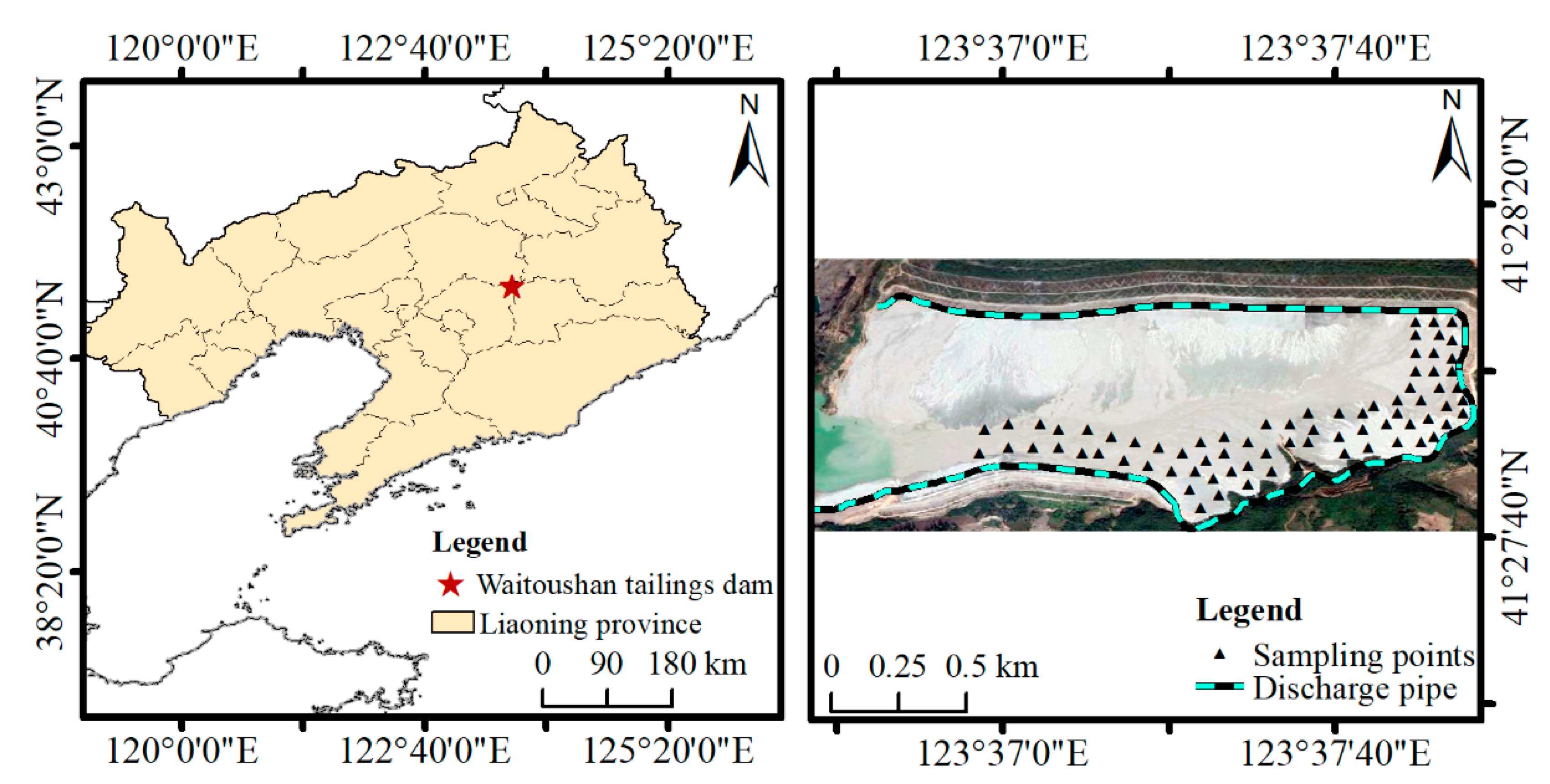
2.1. Tailing Sample Collection

The Waitoushan iron ore tailing dam, which is one of the extra-large iron deposits in the Anshan–Benxi iron cluster of Northeast China, was selected as the study area. The area is located in the north of Benxi, Liaoning Province, Northeast China (Figure 1). The coverage area of the tailing dam is approximately 1.1 km2, with a length of 1.87 km from east to west and a width of 0.85 km from north to south. Tailing pipes are distributed at the southern, eastern, and northern edges of the tailing dam. The tailings are all sourced from the Waitoushan concentrator.
Field surveys were conducted in July 2020. To make the collected samples representative, sampling points were randomly placed along the eastern and southern outlets. A total of 75 tailing samples, each weighing approximately 300 g, were collected with a 100 m3 ring knife of dimensions 79.8 mm× 20 mm on the surface of the tailing dam. The samples were oven-dried, ground, and sieved into a maximum size of 0.075 mm.
X-ray fluorescence spectroscopy was performed to determine the chemical composition of 75 tailing samples. As shown in Figure 2, the main chemical compounds of the tailing samples consist of SiO2, MgO, CaO, and Al2O3, as well as iron cations Fe2+ and Fe3+. The SiO2 content is the highest, with an average proportion of 65.67%, followed by TFe, with an average proportion of 11.63%. All of the tailing samples were divided into 75% for training and 25% for validation.

2.2. Spectral Measurement

The reflectance spectra of the tailing samples were measured by the SVC HR-1024 spectrometer in the wavelength range of 350–2500 nm under laboratory conditions. The tailing samples were placed in a Petri dish with a depth of 3–4 cm, and the surface was leveled to reduce roughness. As the light source, a 50 W halogen bulb was placed at a zenith angle of 30° and 50 cm away from the sample. The sample was measured in a perpendicular direction by the spectrometer with a 4° field-of-view at approximately 47 cm. A Spectralon white plate with 100% reflectance was used for obtaining the reference spectrum. The average of four reflectance spectra per sample was considered as the spectra of the samples.
The TIR spectra were measured by the Turbo FT spectrometer designed by Design & Prototypes Corporation, USA. This spectrometer covers a wavelength range of 2–16 μm with a spectral resolution of 4 cm−1. The sample was measured in the perpendicular direction by the spectrometer with a 4.8° field-of-view at approximately 50 cm. To obtain the spectral emissivity of the tailing samples, it is necessary to measure the cold black-body, hot black-body, atmospheric downward, and sample surface radiance. The atmospheric downward radiation data were collected from a diffuse reflection gold plate. The cold and hot black bodies were used to calibrate the sample surface radiance and atmospheric downward radiance [43]. The sample surface radiance value was the average of two observations of each sample.
The atmospheric window in the 8–13 μm band is relatively less affected by atmospheric radiation and contains the characteristic interval of the quartz emissivity spectrum [44]. Therefore, in this study, the spectral characteristics of the tailing samples were analyzed in the wavelength range of 8–13 μm.

2.3. Data Preprocessing Method

The reflectance spectral data were preprocessed using the Savitzky–Golay (S–G) smoothing method [45], which could reduce the error of data analysis and the random noise generated during the spectral measurement. Subsequently, the measured spectral reflectance (R) was converted into the apparent absorbance (Equation (1)) of the sample to linearize and enhance the correlation between the target parameter concentration and the spectra [46]. Finally, the absorbance data were resampled to 25 nm.
A i = log 10 ( 1 / R i )
where Ai is the absorbance of the sample at band i, and Ri is the spectral reflectance of the sample at band i.
According to Kirchhoff’s law and the theory of atmospheric radiation transmission for natural objects, the total energy detected by the sensor includes: Atmospheric absorption, atmospheric radiation, the reflection of object surface on the radiant energy of surrounding objects, and the incident solar energy. The atmospheric upward radiation can be overlooked when detecting objects at a close range. Therefore, the spectral radiance detected by the sensor at temperature Ts can be approximately expressed as follows [47,48]:
L s ( λ ) = ε s ( λ ) B ( λ , T s ) + [ 1 ε s ( λ ) ] L D W R ( λ )
where Ls(λ) is the calibrated radiance of the sample, εs(λ) is the surface emissivity of the sample, B(λ,Ts) is the Planck function at the sample temperature, and LDWR(λ) is the atmospheric downward radiation.
The emissivity can be computed by transforming Equation (2) as follows:
ε s ( λ ) = L s ( λ ) L D W R ( λ ) B ( λ , T s ) L D W R ( λ )
According to Kirchhoff’s law for opaque objects, the surface reflectance can be expressed as 1 minus the emissivity given by Equation (3). From this perspective, the emissivity was converted to reflectance data, and the absorbance was calculated by Equation (1).

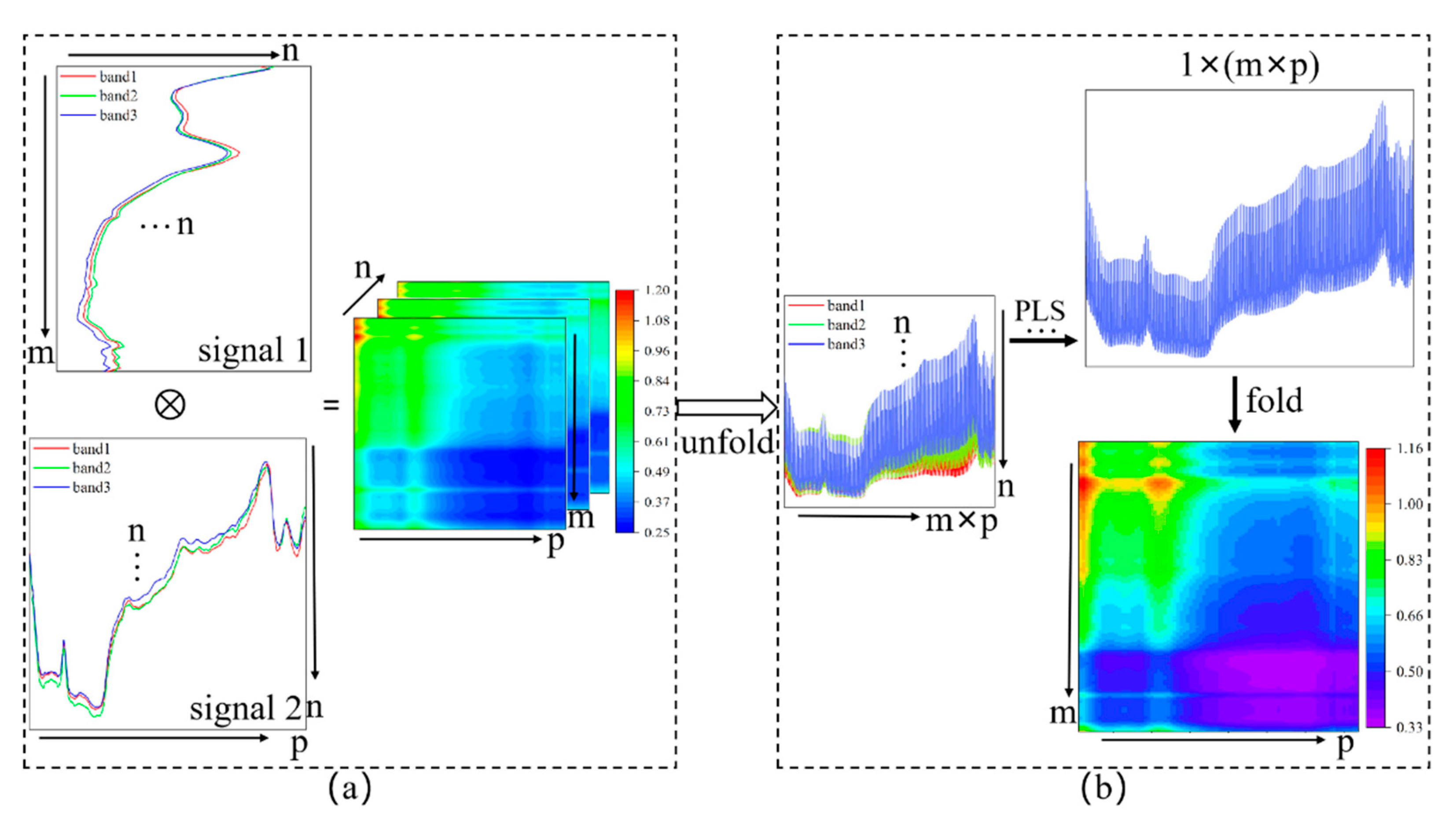
2.4. Spectral Fusion Method

OPA, a notion which was introduced by Barros et al. [24] in 2008, emphasizes the coevolution of spectral regions in signals obtained from different or from the same domains. The outer product (OP) matrix is composed of all possible products of absorbance intensities in the two domains. The calculation process of OPA is shown in Figure 3. For n samples, all absorbance intensities of VIS–NIR spectra (signal 1 of length m) are multiplied by all absorbance intensities of TIR spectra (signal 2 of length p) to generate n (m rows by p columns) matrices, whose absorbance intensities are determined by the intensities of the original spectrum. Subsequently, each matrix is unfolded to a vector and concatenated to produce an n × (m × p) matrix, called the OP matrix. The OP matrix with mean absorbance intensities can be folded back to produce an m × p matrix, Z, which is used to explain the relationship between the two signals and evaluate their coevolution.

2.5. Spectroscopic Modeling Method

PLSR is a linear modeling technique that has been used extensively for chemometrics and quantitative spectroscopy [49]. In this technique, predictor and observed variables are projected into a new space to determine an optimal linear regression model. PLSR can consider the relationship between spectral data and chemical composition simultaneously [50]. In this study, X is the spectrum matrix and Y is the chemical composition, and they are decomposed by PLSR as follows:
X = T P + E x Y = U Q + F y
where T and U are the characteristic factor matrices extracted from X and Y, respectively, P and Q are the load matrices, and Ex and Fy are the error matrices of X and Y, respectively.
The relation in terms of the original space can be expressed as follows:
U = T B + E d
where B and Ed are the matrices of the regression coefficient and residuals, respectively. This regression model was implemented using the “pls” package in R version 3.6.3.
RF is an ensemble classifier based on decision trees and was proposed by Leo Breiman and Adele Cutler in 2001 [51]. For predicting the content of tailings, RF obtains multiple bootstrap datasets through multiple random and repeatable extractions from the original training set. A decision tree is constructed for each bootstrap dataset, and the average of the predicted values of all decision trees is used as the predicted value of the RF model. The parameters of the RF model are comparatively simple to set. RF runs faster with high classification accuracy and better stability when using high-dimensional data for prediction. The RF regression model in this study was built using the “TreeBagger” function in MATLAB software, and the number of trees was set to 500.
ELM [52] is a machine learning algorithm based on a single hidden layer feedforward neural network (SLFN). This algorithm has the advantages of high calculation speed and requirement of fewer training parameters. However, due to the fact that ELM randomly selects the input weight and hidden layer bias, the accuracy of ELM is generally low [39,40,41]. PSO is a population-based stochastic optimization technique that simulates the social behavior of a flock of birds or a school of fish [53,54]. The input weight and hidden layer bias of ELM optimized using the PSO can effectively reduce the number of hidden layer nodes required by the ELM, thereby improving the calculation efficiency and the generalizability of a trained neural network. In this study, the PSO–ELM regression model was realized by MATLAB, with the maximum number of iterations set to 100 and the number of hidden layer nodes set to 5. The inertia weights ωwin and ωmax were set to 0.4 and 0.8, and the learning rates c1 and c2 were set to 2.4 and 1.6, respectively.
The performance of the models was evaluated in terms of R2, root mean square error (RMSE), and ratio of performance to interquartile distance (RPIQ). The RPIQ is based on the quartile distance and better represents the spread of the population for skewed distributions. Therefore, it is used rather than the ratio of performance deviation [55,56].
R 2 = i = 1 n ( y ^ i y ¯ ) 2 i = 1 n ( y i y ¯ ) 2
R M S E = 1 n i = 1 n ( y i y ^ i ) 2
R P I Q = I Q R M S E I Q = Q 3 Q 1
Here, n is the number of samples, y i ^ is the predicted value, y i is the measured value, y ¯ is the average value, Q3 is the third quartile, and Q1 is the first quartile. In general, a robust model has a high R² and RPIQ and a low RMSE.

3. Results and Discussion

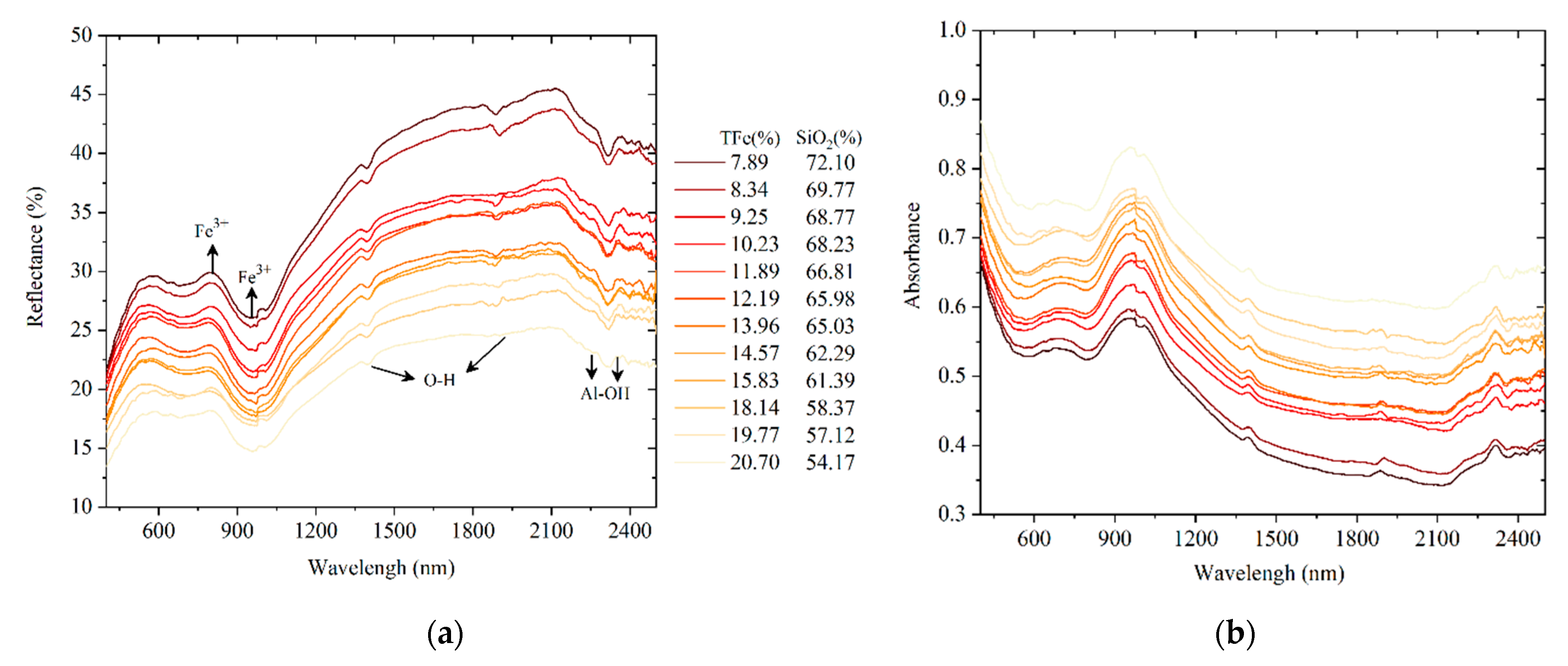
3.1. VIS–NIR Spectral and Absorption Characteristics

The TFe and SiO2 content in the tailing samples ranged from 7.78%–20.7% and 54.17%–72.1%, respectively. All of the samples were divided into 12 grades, according to the TFe and SiO2 content. The VIS–NIR reflectance and absorbance spectra of the tailing samples, respectively are shown in Figure 4a,b. In Figure 4a, the samples with higher SiO2 content and lower TFe content resulted in higher reflectance. The absorption peaks observed near 750 and 980 nm were due to electronic transitions in minerals containing Fe3+ (e.g., goethite and hematite) [57,58]. This characteristic gradually increased from 1000 to 2100 nm. The absorbance peaks at 1450 and 1950 nm could be related to the combination of stretching and bending vibrations of the hydroxyl group (O–H) in water molecules [59,60,61]. The absorption characteristics at 2250 and 2350 nm are usually attributed to the aluminol group (Al–OH) [13,15,62].

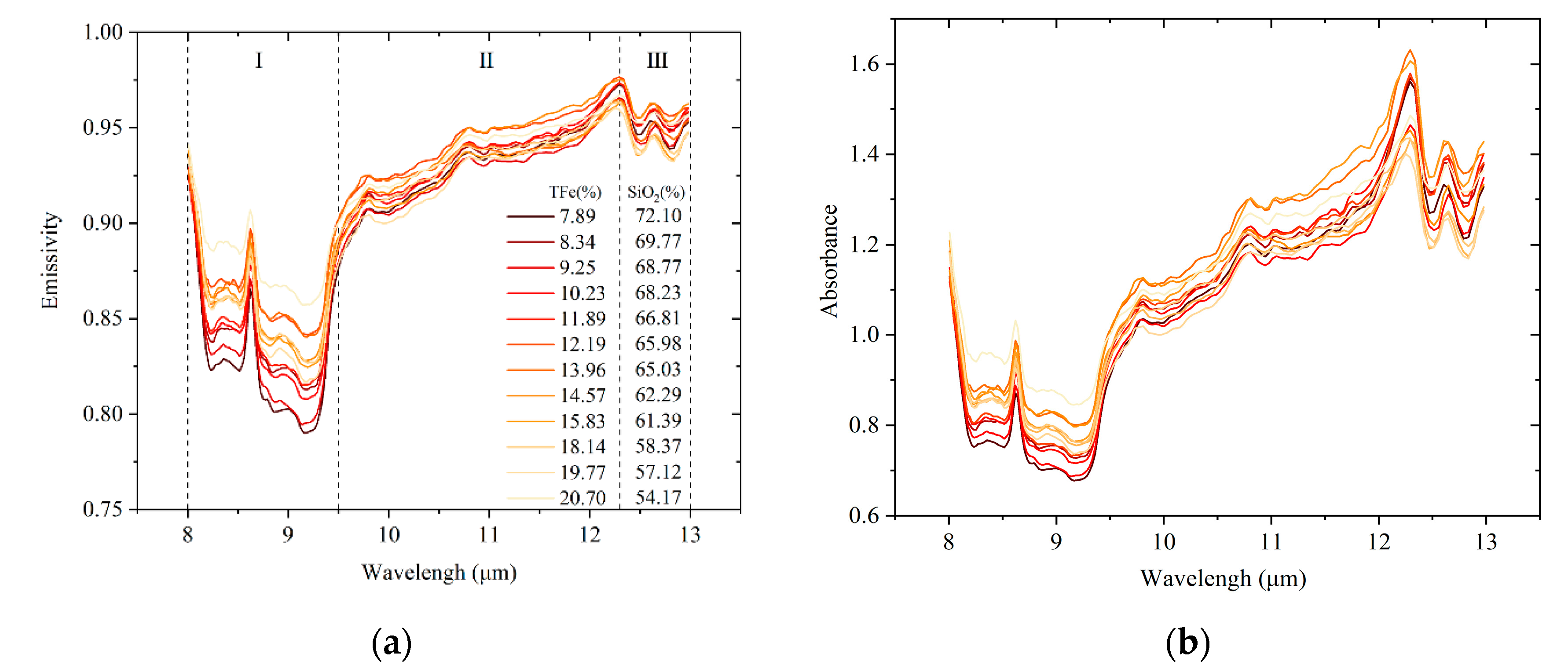
3.2. TIR Spectral and Absorption Characteristics

The TIR reflectance and absorbance spectra of the tailing samples, respectively are shown in Figure 5a,b. In Figure 5a, the emissivity spectra in the TIR range with higher TFe content and lower SiO2 content result in higher emissivity. All of the emissivity spectra in the TIR range were divided into three regions. In region I (8–9.5 μm), the absorption characteristics are distinct, forming two asymmetric absorption bands near 8.6 μm, which were attributed to the stretching vibration of the Si–O bond [63]. The spectral absorption depth gradually increased with the increasing SiO2 content. In region II (9.5–12.3 μm), the emissivity increased evidently, and there was no significant relationship between SiO2 content and reflectance. In region III (12.3–13 μm), two weak absorption peaks due to the Si–O–Si symmetric stretching vibration were observed. However, this characteristic was not significantly correlated with SiO2 content [64].

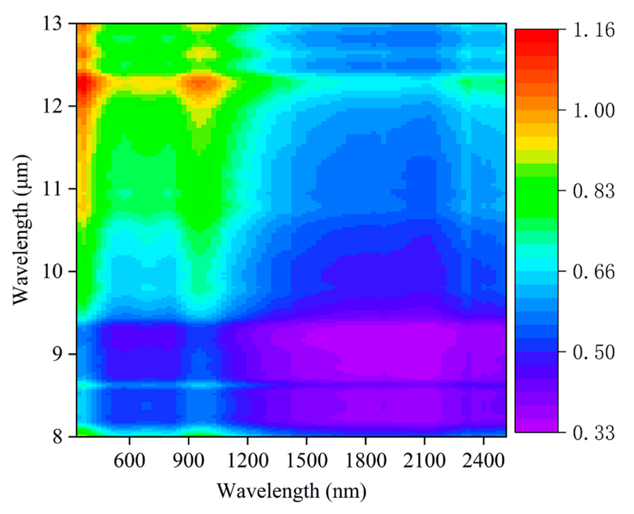
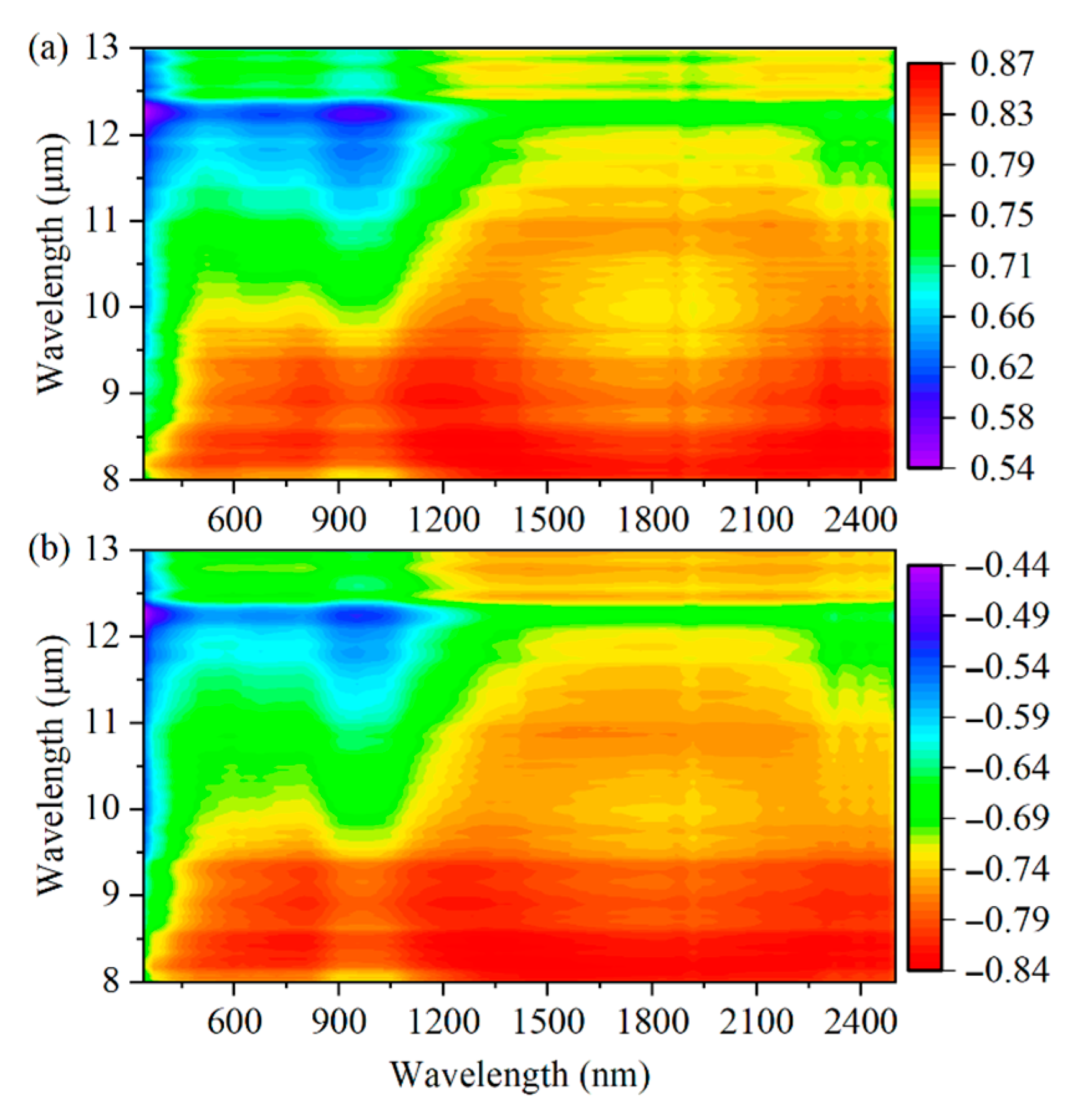
3.3. Spectral Data Fusion and Coevolution

In applying spectral data fusion, the absorbance intensities of the TIR spectral data (168 bands) were multiplied by all the absorbance intensities of the VIS–NIR spectral data (86 bands), generating a matrix with 14,448 bands (168 × 86). The OP matrix formed with the mean intensities is shown in Figure 6. The X- and Y-axes represent the wavelengths of the VIS–NIR and TIR spectra, respectively. Higher absorbance intensities of the fused spectra are distributed in the ranges of 350–1200 nm in the VIS–NIR region and 10.7–13 μm in the TIR region, indicated by red in the color bar.

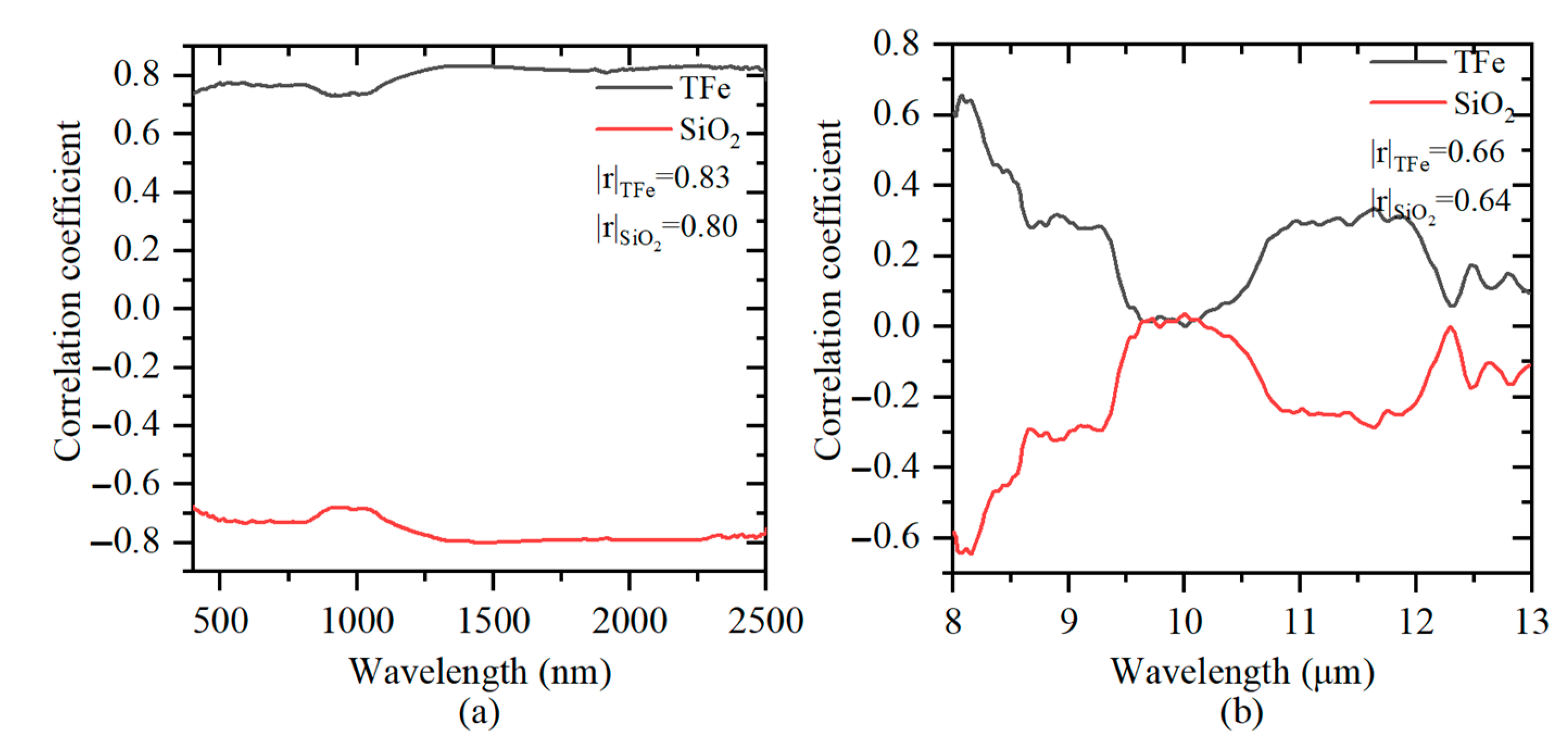
3.4. Correlation of Spectral Data with TFe and SiO2 Content

In the VIS–NIR region, absorbance intensity was positively correlated with TFe content (Figure 7a), with the highest correlation coefficient of 0.83 recorded in the range of 1163–2499 nm. By contrast, a negative correlation was observed between SiO2 content and absorbance intensity, with the highest correlation coefficient of 0.80 recorded in the ranges of 1365–1391 nm and 1410–1623 nm. In the TIR region, absorbance intensity was positively correlated with TFe content, with the highest correlation coefficient of 0.66 recorded in the ranges of 8–9.4 μm and 10.7–12 μm, but negatively correlated with SiO2 content, with the highest correlation coefficient of 0.64 recorded in the same range (Figure 7b).
The Pearson correlation calculations were performed to analyze the fused absorbance data in relation to TFe and SiO2. The correlation of fused absorbances with TFe and SiO2 is shown in Figure 8. In the fused matrix, absorbance intensity was positively correlated with TFe content (Figure 8a) and negatively correlated with SiO2 content (Figure 8b). The fused spectra significantly correlated with TFe and SiO2 contents (|r|≥ 0.80). The fusion domain (1181–1409 nm and 2298–2375 nm for VIS–NIR, 8.17–8.27 μm and 8.37–8.52 μm for TIR) had the largest correlation coefficient of 0.87 with TFe content. The largest correlation coefficient between the fusion domain (1257–1714 nm for VIS–NIR and 8.13–0.54 μm for TIR) and SiO2 content was 0.84. The fused spectra showed a significantly improved correlation of TIR absorbance with TFe from 0.66 to 0.87 and SiO2 from 0.64 to 0.84. However, the improvement effect of the VIS–NIR absorbance correlation with TFe and SiO2 was not evident. This indicates that the fused data can effectively improve the correlation of absorbance with TFe and SiO2 compared with the individual spectral. A similar result was demonstrated in a previous study, in which SOC more strongly correlated with the OPA-fused spectral domain using VIS–NIR and TIR spectroscopy than with the individual spectral domains [29].

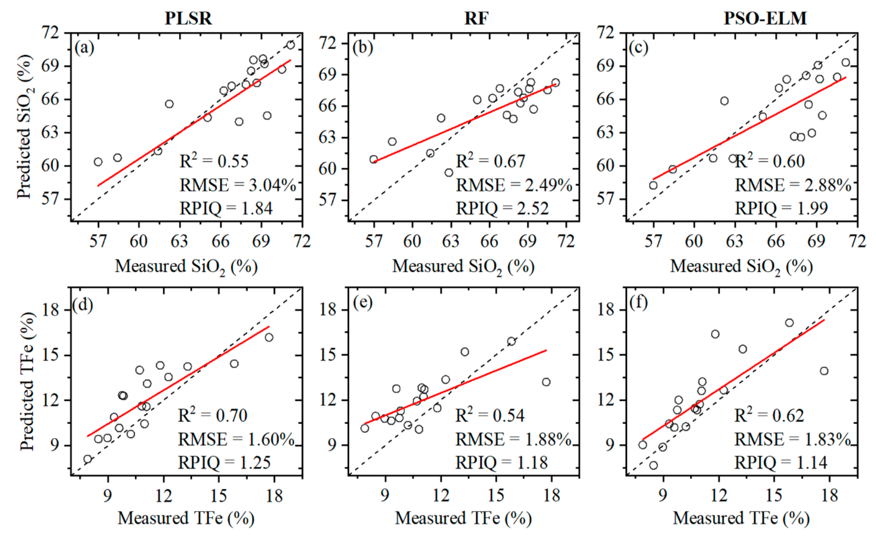
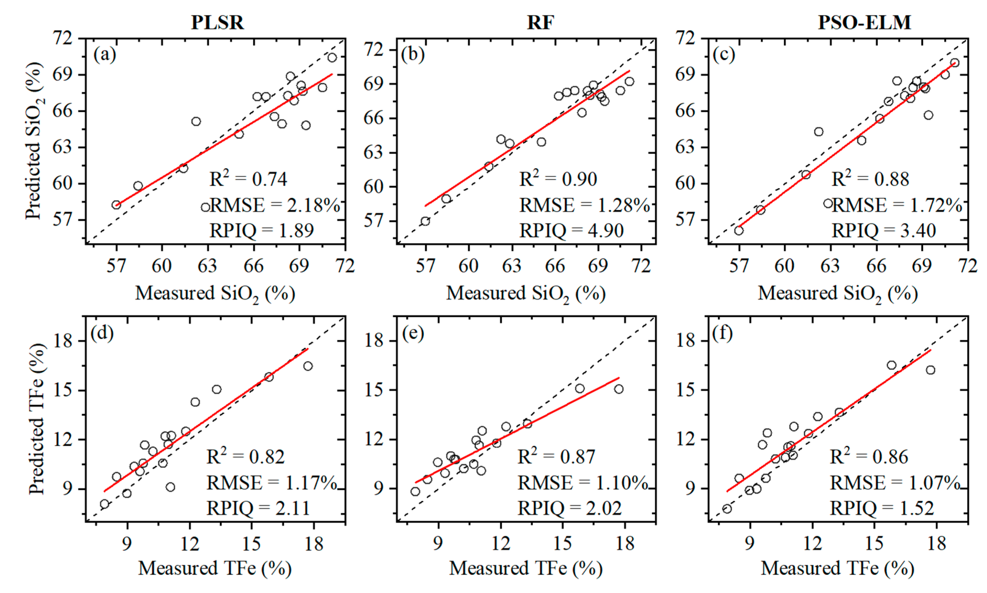
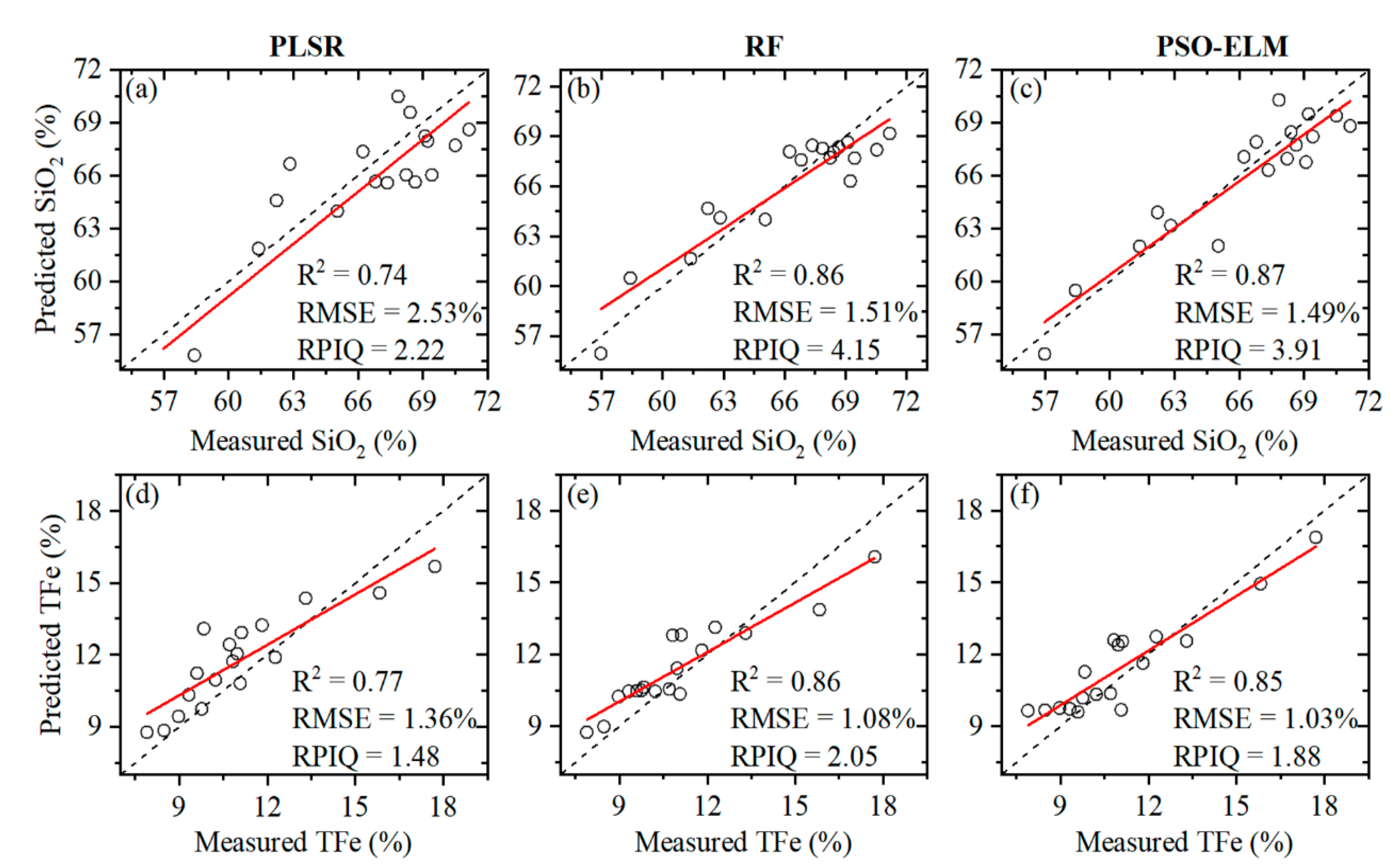
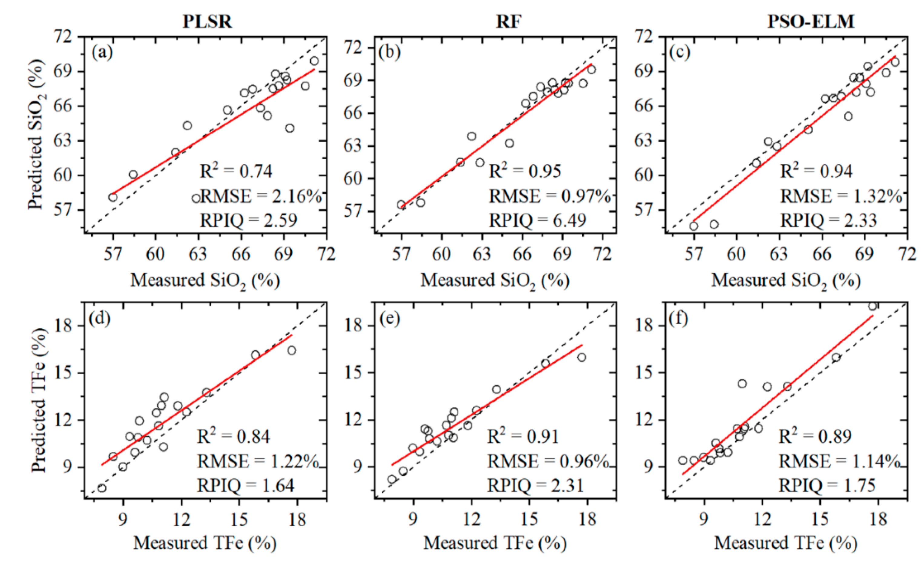
3.5. Prediction Accuracy of TFe and SiO2

To compare OPA with the data augmentation method, we combined the absorbance data of VIS–NIR and TIR to generate an n × (m + p) matrix to predict the accuracy of TFe and SiO2. The prediction accuracy of TFe and SiO2 using PLSR, RF, and PSO–ELM regression methods based on different input spectra (VIS–NIR, TIR, data augmentation, and OPA-fused) is presented in Table 1. Notably, all of the results presented in the table are obtained from the test dataset. A different balance of training and validation samples could be applied, and it was reasonable to use around 25% of the samples for validation [65]. In this paper, the samples were all randomly divided into 57 training samples and 18 validation samples. In the VIS–NIR domain, the input spectra with ranges of 1163–2499 nm for TFe content and 1365–1391 nm and 1410–1623 nm for SiO2 content were selected on the basis of the correlation analysis to develop multivariate regression models by PLSR, RF, and PSO–ELM. As shown in Figure 9, the RF and PSO–ELM models performed better than the PLSR model with the VIS–NIR spectral data. In terms of TFe prediction, the RF model showed the highest prediction capability with the validation criteria R2 = 0.86, RMSE = 1.08%, and RPIQ = 2.05. For SiO2 prediction, the PSO–ELM model performed the best with R2 = 0.87, RMSE = 1.49%, and RPIQ = 3.91.
In the TIR domain, the input spectra with ranges of 8–9.4 μm and 10.7–12 μm were selected to establish TFe and SiO2 prediction models. As shown in Figure 10, the most accurate predictions were obtained with the PLSR model for TFe (R2 = 0.70, RMSE = 1.60%, and RPIQ = 1.25) and the RF model for SiO2 (R2 = 0.67, RMSE = 2.49%, and RPIQ = 2.52).
In the fused domain, the spectral absorbance intensities that were significantly correlated with TFe and SiO2 (|r| ≥ 0.80) were selected for achieving the regression models. As shown in Figure 12, the RF model produced the best prediction for TFe and SiO2 with R2 = 0.91 and 0.95, RMSE = 0.96% and 0.97%, and RPIQ = 2.31 and 6.49, respectively. The OPA-fused spectra produced statistically better results than VIS–NIR, TIR, and data augmentation spectra. For TFe prediction, the R2 value increased from 0.70 to 0.91, RMSE decreased from 1.60% to 0.96%, and RPIQ increased from 1.25 to 2.31. For SiO2 prediction, the R2 value increased from 0.67 to 0.95, RMSE decreased from 2.49% to 0.97%, and RPIQ increased from 2.52 to 6.49. This implies that OPA fusion for combining VIS–NIR and TIR spectra is an effective approach for estimating TFe and SiO2 content and can extend the order of magnitude of the prediction for TFe and SiO2 content. The data augmentation spectra retained all of the absorbance intensity information of VIS–NIR and TIR, improving the prediction accuracy of TFe and SiO2 content compared with individual VIS–NIR and TIR spectra. Compared with data augmentation, OPA fusion spectra expanded the possibility of finding a spectral coevolution that was more relevant to TFe and SiO2 [24,29,66]. Compared with previous studies that use OPA to fuse VIS–NIR and MIR spectra [28,29], this study achieved significant improvement in fusing VIS–NIR and TIR spectral data for TFe and SiO2 prediction, thus indicating that OPA takes full advantage of the different characteristics and complementary information of the two spectra. OPA-fused spectroscopy using VIS–NIR and TIR input data can serve as a stable and effective method for TFe and SiO2 prediction. It can be seen that in four different input ways with single VIS–NIR, single TIR, data augmentation, and OPA-fused, the lower RMSE value of TFe was generated rather than the value of SiO2. This was similar to Desta et al. [21], who found that the lower RMSE of Fe2O3 (RMSE = 3.3%) was achieved using the PLSR model combined with the MWIR and LWIR concatenation data compared with SiO2 (RMSE = 5.96%).
The results of this study indicated that the RF model performs better than PLSR and PSO–ELM models for TFe and SiO2 estimation using OPA-fused spectra. Bao et al. [67] verified that the RF model could produce superior results compared with the PLSR and SVM models for predicting the soil organic matter content in reclaimed mine soil. In addition, the RF model considers only the most important variables in the input spectra, thereby significantly reducing the risk of model overfitting and dampening the effects of noise and outliers [51,68,69,70,71]. Compared with other machine learning methods, RF deliberately generates a large number of decision trees by randomly selecting subsets of training samples and variables for segmentation at each tree node [72]. Therefore, the RF model is less sensitive to the quality of training samples and to overfitting. Owing to this characteristic of RF modeling, improved results can be obtained for the regression prediction of tailing component contents using hyperspectral data.

4. Conclusions

This study proposed the combined VIS–NIR and TIR spectroscopy coupled with a machine learning method to effectively quantify the contents of TFe and SiO2 in high-silicon iron tailings. OPA can fuse VIS–NIR and TIR spectra to improve predictions of TFe and SiO2. The following conclusions can be drawn from the study:
  • This study demonstrated that with the VIS–NIR spectra, the sensitive absorption bands of SiO2 occurred in the ranges of 1365–1391 nm and 1410–1623 nm, and those of TFe occurred in the range of 1163–2499 nm. In the TIR domain, the sensitive absorption bands of both SiO2 and TFe were in the ranges of 8–9.4 μm and 10.7–12 μm.
  • Compared with individual VIS–NIR or TIR spectra, the OPA-fused absorbance data had a stronger correlation with TFe and SiO2 content. The largest correlation coefficient between TFe and the fusion domain (1181–1409 nm and 2298–2375 nm for VIS–NIR, 8.17–8.27 μm, and 8.37–8.52 μm for TIR) was 0.87. By contrast, the largest correlation coefficient between SiO2 and the fusion domain (1257–1714 nm for VIS–NIR and 8.13–0.54 μm for TIR) was 0.84.
  • The combination of RF modeling and OPA-fused spectral data achieved the optimal prediction accuracy of TFe and SiO2 compared with the accuracy obtained through individual spectra. The R2 value increased from 0.70 to 0.91, RMSE decreased from 1.60% to 0.96%, and RPIQ increased from 1.25 to 2.31 for TFe prediction. The R2 value increased from 0.67 to 0.95, RMSE decreased from 2.49% to 0.97%, and RPIQ increased from 2.52 to 6.49 for SiO2 prediction. The RF model performed better than the PLSR and PSO–ELM models, with greater R2 and RPIQ and lower RMSE values.

Author Contributions

Conceptualization, N.B.; writing—original draft preparation, H.L.; software, Y.C.; writing—review and editing, N.B. and S.L.; supervision, X.G. and B.Z.; funding acquisition, N.B., Y.F., X.G. and B.Z. All authors have read and agreed to the published version of the manuscript.

Funding

This research was funded by the National Natural Science Foundation of China, grant number 52074063 and 52074064, Major Special Project of Science and Technology Plan, grant number 2020020307-JH1/103-02, Fundamental Research Funds for the Central Universities, grant number N2001002, 2021 Liaoning Provincial People’s Livelihood Science and Technology Project, grant number 2021JH2/10200035.

Data Availability Statement

Not applicable.

Acknowledgments

We acknowledge the analysis and testing center of Northeastern University Research Institute for measuring the content of tailings.

Conflicts of Interest

The authors declare no conflict of interest.

References

  1. Burritt, R.L.; Christ, K.L. Water risk in mining: Analysis of the samarco dam failure. J. Clean. Prod. 2018, 178, 196–205. [Google Scholar] [CrossRef]
  2. Kossoff, D.; Dubbin, W.; Alfredsson, M.; Edwards, S.; Macklin, M.; Hudson-Edwards, K.A. Mine tailings dams: Characteristics, failure, environmental impacts, and remediation. Appl. Geochem. 2014, 51, 229–245. [Google Scholar] [CrossRef] [Green Version]
  3. Zhang, Z.; Hou, T.; Santosh, M.; Li, H.; Li, J.; Zhang, Z.; Song, X.; Wang, M. Spatio-temporal distribution and tectonic settings of the major iron deposits in China: An overview. Ore Geol. Rev. 2014, 57, 247–263. [Google Scholar] [CrossRef]
  4. Wan, Y.; Hu, X.; Zhong, Y.; Ma, A.; Wei, L.; Zhang, L. In Tailings reservoir disaster and environmental monitoring using the uav-ground hyperspectral joint observation and processing: A case of study in Xinjiang, the belt and road. In Proceedings of the IGARSS 2019—2019 IEEE International Geoscience and Remote Sensing Symposium, Yokohama, Japan, 28 July–2 August 2019; IEEE: Manhattan, NY, USA; pp. 9713–9716. [Google Scholar]
  5. Dong, L.; Deng, S.; Wang, F. Some developments and new insights for environmental sustainability and disaster control of tailings dam. J. Clean. Prod. 2020, 269, 122270. [Google Scholar] [CrossRef]
  6. Lyon, R. Analysis of rocks by spectral infrared emission (8 to 25 microns). Econ. Geol. 1965, 60, 715–736. [Google Scholar] [CrossRef]
  7. Yang, X.; Bao, N.; Li, W.; Liu, S.; Fu, Y.; Mao, Y. Soil nutrient estimation and mapping in farmland based on uav imaging spectrometry. Sensors 2021, 21, 3919. [Google Scholar] [CrossRef]
  8. Ben-Dor, E.; Inbar, Y.; Chen, Y. The reflectance spectra of organic matter in the visible near-infrared and short wave infrared region (400–2500 nm) during a controlled decomposition process. Remote Sens. Environ. 1997, 61, 1–15. [Google Scholar] [CrossRef]
  9. Abrams, M.; Rothery, D.; Pontual, A. Mapping in the oman ophiolite using enhanced landsat thematic mapper images. Tectonophysics 1988, 151, 387–401. [Google Scholar] [CrossRef]
  10. Xiao, D.; Liu, C.; Le, B.T. Detection method of tfe content of iron ore based on visible-infrared spectroscopy and ipso-telm neural network. Infrared Phys. Technol. 2019, 97, 341–348. [Google Scholar] [CrossRef]
  11. Bishop, J.L.; Dyar, M.D.; Lane, M.D.; Banfield, J.F. Spectral identification of hydrated sulfates on mars and comparison with acidic environments on earth. Int. J. Astrobiol. 2004, 3, 275–285. [Google Scholar] [CrossRef] [Green Version]
  12. Johnson, J.; Bell, J.F., III; Cloutis, E.; Staid, M.; Farrand, W.; McCoy, T.; Rice, M.; Wang, A.; Yen, A. Mineralogic constraints on sulfur-rich soils from Pancam spectra at Gusev crater, Mars. Geophys. Res. Lett. 2007, 34, 1–6. [Google Scholar] [CrossRef]
  13. Michalski, J.R.; Cuadros, J.; Bishop, J.L.; Dyar, M.D.; Dekov, V.; Fiore, S. Constraints on the crystal-chemistry of Fe/Mg-rich smectitic clays on Mars and links to global alteration trends. Earth Planet. Sci. Lett. 2015, 427, 215–225. [Google Scholar] [CrossRef] [Green Version]
  14. Carter, J.; Poulet, F.; Bibring, J.P.; Mangold, N.; Murchie, S. Hydrous minerals on Mars as seen by the CRISM and OMEGA imaging spectrometers: Updated global view. J. Geophys. Res. Planets 2013, 118, 831–858. [Google Scholar] [CrossRef]
  15. Sánchez-Marañón, M.; Cuadros, J.; Michalski, J.R.; Melgosa, M.; Dekov, V. Identification of iron in Earth analogues of Martian phyllosilicates using visible reflectance spectroscopy: Spectral derivatives and color parameters. Appl. Clay Sci. 2018, 165, 264–276. [Google Scholar] [CrossRef]
  16. Cuadros, J.; Michalski, J.R.; Bishop, J.L.; Mavris, C.; Fiore, S.; Dekov, V. Mars-rover cameras evaluation of laboratory spectra of Fe-bearing Mars analog samples. Icarus 2022, 371, 114704. [Google Scholar] [CrossRef]
  17. Cuadros, J.; Sánchez-Marañón, M.; Mavris, C.; Fiore, S.; Bishop, J.L.; Melgosa, M. Color analysis and detection of Fe minerals in multi-mineral mixtures from acid-alteration environments. Appl. Clay Sci. 2020, 193, 105677. [Google Scholar] [CrossRef]
  18. Wang, D.; Liu, S.-J.; Mao, Y.-C.; Wang, Y.; Li, T.-Z. A Method Based on Thermal Infrared Spectrum for Analysis of SiO2 Content in Anshan-Type Iron. Spectrosc. Spectr. Anal. 2018, 38, 2101–2106. [Google Scholar] [CrossRef]
  19. Song, L.; Liu, S.; Li, W. Quantitative inversion of fixed carbon content in coal gangue by thermal infrared spectral data. Energies 2019, 12, 1659. [Google Scholar] [CrossRef] [Green Version]
  20. Song, L.; Liu, S.; Yu, M.; Mao, Y.; Wu, L. A classification method based on the combination of visible, near-infrared and thermal infrared spectrum for coal and gangue distinguishment. Spectrosc. Spectr. Anal. 2017, 37, 416–422. [Google Scholar]
  21. Desta, F.; Buxton, M.; Jansen, J. Fusion of mid-wave infrared and long-wave infrared reflectance spectra for quantitative analysis of minerals. Sensors 2020, 20, 1472. [Google Scholar] [CrossRef] [Green Version]
  22. Ng, W.; Minasny, B.; Montazerolghaem, M.; Padarian, J.; Ferguson, R.; Bailey, S.; McBratney, A.B. Convolutional neural network for simultaneous prediction of several soil properties using visible/near-infrared, mid-infrared, and their combined spectra. Geoderma 2019, 352, 251–267. [Google Scholar] [CrossRef]
  23. Jaillais, B.; Pinto, R.; Barros, A.S.; Rutledge, D.N. Outer-product analysis (OPA) using PCA to study the influence of temperature on NIR spectra of water. Vib. Spectrosc. 2005, 39, 50–58. [Google Scholar] [CrossRef]
  24. Barros, A.S.; Pinto, R.; Bouveresse, D.J.-R.; Rutledge, D.N. Principal component transform—Outer product analysis in the PCA context. Chemom. Intell. Lab. Syst. 2008, 93, 43–48. [Google Scholar] [CrossRef]
  25. Di Natale, C.; Zude-Sasse, M.; Macagnano, A.; Paolesse, R.; Herold, B.; D’Amico, A. Outer product analysis of electronic nose and visible spectra: Application to the measurement of peach fruit characteristics. Anal. Chim. Acta 2002, 459, 107–117. [Google Scholar] [CrossRef]
  26. Jaillais, B.; Morrin, V.; Downey, G. Image processing of outer-product matrices–A new way to classify samples: Examples using visible/NIR/MIR spectral data. Chemom. Intell. Lab. Syst. 2007, 86, 179–188. [Google Scholar] [CrossRef]
  27. Maalouly, J.; Eveleigh, L.; Rutledge, D.N.; Ducauze, C.J. Application of 2D correlation spectroscopy and outer product analysis to infrared spectra of sugar beets. Vib. Spectrosc. 2004, 36, 279–285. [Google Scholar] [CrossRef]
  28. Cécillon, L.; Certini, G.; Lange, H.; Forte, C.; Strand, L.T. Spectral fingerprinting of soil organic matter composition. Org. Geochem. 2012, 46, 127–136. [Google Scholar] [CrossRef]
  29. Terra, F.S.; Viscarra Rossel, R.A.; Demattê, J.A.M. Spectral fusion by Outer Product Analysis (OPA) to improve predictions of soil organic C. Geoderma 2019, 335, 35–46. [Google Scholar] [CrossRef]
  30. Rossel, R.V.; Walvoort, D.; McBratney, A.; Janik, L.J.; Skjemstad, J. Visible, near infrared, mid infrared or combined diffuse reflectance spectroscopy for simultaneous assessment of various soil properties. Geoderma 2006, 131, 59–75. [Google Scholar] [CrossRef]
  31. Summers, D.; Lewis, M.; Ostendorf, B.; Chittleborough, D. Visible near-infrared reflectance spectroscopy as a predictive indicator of soil properties. Ecol. Indic. 2011, 11, 123–131. [Google Scholar] [CrossRef]
  32. Wang, S.; Guan, K.; Zhang, C.; Lee, D.; Margenot, A.J.; Ge, Y.; Peng, J.; Zhou, W.; Zhou, Q.; Huang, Y. Using soil library hyperspectral reflectance and machine learning to predict soil organic carbon: Assessing potential of airborne and spaceborne optical soil sensing. Remote Sens. Environ. 2022, 271, 112914. [Google Scholar] [CrossRef]
  33. Kopačková-Strnadová, V.; Rapprich, V.; McLemore, V.; Pour, O.; Magna, T. Quantitative estimation of rare earth element abundances in compositionally distinct carbonatites: Implications for proximal remote-sensing prospection of critical elements. Int. J. Appl. Earth Obs. Geoinf. 2021, 103, 102423. [Google Scholar] [CrossRef]
  34. Sun, W.; Liu, S.; Zhang, X.; Li, Y. Estimation of soil organic matter content using selected spectral subset of hyperspectral data. Geoderma 2022, 409, 115653. [Google Scholar] [CrossRef]
  35. Li, H.; Liang, Y.; Xu, Q.; Cao, D. Key wavelengths screening using competitive adaptive reweighted sampling method for multivariate calibration. Anal. Chim. Acta 2009, 648, 77–84. [Google Scholar] [CrossRef] [PubMed]
  36. Gholizadeh, A.; Borůvka, L.; Saberioon, M.; Vašát, R. Visible, near-infrared, and mid-infrared spectroscopy applications for soil assessment with emphasis on soil organic matter content and quality: State-of-the-art and key issues. Appl. Spectrosc. 2013, 67, 1349–1362. [Google Scholar] [CrossRef] [PubMed]
  37. Pal, M. Random forest classifier for remote sensing classification. Int. J. Remote Sens. 2005, 26, 217–222. [Google Scholar] [CrossRef]
  38. Figueiredo, E.M.; Ludermir, T.B. Investigating the use of alternative topologies on performance of the PSO-ELM. Neurocomputing 2014, 127, 4–12. [Google Scholar] [CrossRef]
  39. Han, F.; Yao, H.-F.; Ling, Q.-H. An improved evolutionary extreme learning machine based on particle swarm optimization. Neurocomputing 2013, 116, 87–93. [Google Scholar] [CrossRef]
  40. Zhao, G.; Shen, Z.; Miao, C.; Man, Z. On improving the conditioning of extreme learning machine: A linear case. In Proceedings of the 2009 7th International Conference on Information, Communications and Signal Processing (ICICS), Macau, China, 8–10 December 2009; pp. 1–5. [Google Scholar]
  41. Zhu, Q.-Y.; Qin, A.K.; Suganthan, P.N.; Huang, G.-B. Evolutionary extreme learning machine. Pattern Recognit. 2005, 38, 1759–1763. [Google Scholar] [CrossRef]
  42. You, X.; Yang, S. In Evolutionary Extreme Learning Machine–Based on Particle Swarm Optimization, Advances in Neural Networks–ISNN 2006. In Proceedings of the Third International Symposium on Neural Networks, Chengdu, China, 28 May 2006. [Google Scholar]
  43. Bao, N.; Liu, S.; Zhou, Y. Predicting particle-size distribution using thermal infrared spectroscopy from reclaimed mine land in the semi-arid grassland of North China. Catena 2019, 183, 104190. [Google Scholar] [CrossRef]
  44. Salisbury, J.W.; D’Aria, D.M. Emissivity of terrestrial materials in the 8–14 μm atmospheric window. Remote Sens. Environ. 1992, 42, 83–106. [Google Scholar] [CrossRef]
  45. Savitzky, A.; Golay, M.J. Smoothing and differentiation of data by simplified least squares procedures. Anal. Chem. 1964, 36, 1627–1639. [Google Scholar] [CrossRef]
  46. Stenberg, B.; Rossel, R.A.V.; Mouazen, A.M.; Wetterlind, J. Visible and near infrared spectroscopy in soil science. Adv. Agron. 2010, 107, 163–215. [Google Scholar]
  47. Ruff, S.W.; Christensen, P.R.; Barbera, P.W.; Anderson, D.L. Quantitative thermal emission spectroscopy of minerals: A laboratory technique for measurement and calibration. J. Geophys. Res. 1997, 102, 14899–14913. [Google Scholar] [CrossRef]
  48. Salvaggio, C.; Miller, C.J. Methodologies and protocols for the collection of midwave and longwave infrared emissivity spectra using a portable field spectrometer. In Proceedings of the Algorithms for Multispectral, Hyperspectral, and Ultraspectral Imagery VII, Orlando, FL, USA, 20 August 2001; pp. 539–548. [Google Scholar]
  49. Wold, S.; Martens, H.; Wold, H. The multivariate calibration problem in chemistry solved by the PLS method. In Matrix Pencils; Springer: Berlin/Heidelberg, Germany, 1983; pp. 286–293. [Google Scholar]
  50. Ben-Dor, E.; Chabrillat, S.; Demattê, J.A.M.; Taylor, G.; Hill, J.; Whiting, M.; Sommer, S. Using imaging spectroscopy to study soil properties. Remote Sens. Environ. 2009, 113, S38–S55. [Google Scholar] [CrossRef]
  51. Breiman, L. Random forests. Mach. Learn. 2001, 45, 5–32. [Google Scholar] [CrossRef] [Green Version]
  52. Huang, G.-B.; Zhu, Q.-Y.; Siew, C.-K. Extreme learning machine: A new learning scheme of feedforward neural networks. In Proceedings of the 2004 IEEE International Joint Conference on Neural Networks (IEEE Cat. No. 04CH37541), Budapest, Hungary, 25–29 July 2004; pp. 985–990. [Google Scholar]
  53. Eberhart, R.; Kennedy, J. A new optimizer using particle swarm theory. In Proceedings of the MHS’95, Sixth International Symposium on Micro Machine and Human Science, Nagoya, Japan, 4–6 October 1995; pp. 39–43. [Google Scholar]
  54. Kennedy, J.; Eberhart, R. Particle swarm optimization. In Proceedings of the ICNN’95 International Conference on Neural Networks, Perth, Australia, 27 November–1 December 1995; pp. 1942–1948. [Google Scholar]
  55. Silva, E.B.; Giasson, É.; Dotto, A.C.; Caten, A.t.; Demattê, J.A.M.; Bacic, I.L.Z.; Veiga, M.d. A regional legacy soil dataset for prediction of sand and clay content with VIS-NIR-SWIR, in southern Brazil. Rev. Bras. Cienc. Solo 2019, 43, 1–20. [Google Scholar] [CrossRef] [Green Version]
  56. Bellon-Maurel, V.; Fernandez-Ahumada, E.; Palagos, B.; Roger, J.-M.; McBratney, A. Critical review of chemometric indicators commonly used for assessing the quality of the prediction of soil attributes by NIR spectroscopy. TrAC Trends Anal. Chem. 2010, 29, 1073–1081. [Google Scholar] [CrossRef]
  57. Bishop, J.; Lane, M.; Dyar, M.; Brown, A. Reflectance and emission spectroscopy study of four groups of phyllosilicates: Smectites, kaolinite-serpentines, chlorites and micas. Clay Miner. 2008, 43, 35–54. [Google Scholar] [CrossRef]
  58. Bishop, J.L.; Pieters, C.M.; Edwards, J.O. Infrared spectroscopic analyses on the nature of water in montmorillonite. Clays Clay Miner. 1994, 42, 702–716. [Google Scholar] [CrossRef]
  59. Crowley, J.K. Visible and near-infrared (0.4–2.5 μm) reflectance spectra of playa evaporite minerals. J. Geophys. Res. 1991, 96, 16231–16240. [Google Scholar] [CrossRef]
  60. Crowley, J.; Williams, D.; Hammarstrom, J.; Piatak, N.; Chou, I.-M.; Mars, J. Spectral reflectance properties (0.4–2.5 μm) of secondary Fe-oxide, Fe-hydroxide, and Fe-sulphate-hydrate minerals associated with sulphide-bearing mine wastes. Geochemistry 2003, 3, 219–228. [Google Scholar] [CrossRef]
  61. Tan, W.; Qin, X.; Liu, J.; Michalski, J.; He, H.; Yao, Y.; Yang, M.; Huang, J.; Lin, X.; Zhang, C. Visible/near infrared reflectance (VNIR) spectral features of ion-exchangeable Rare earth elements hosted by clay minerals: Potential use for exploration of regolith-hosted REE deposits. Appl. Clay Sci. 2021, 215, 106320. [Google Scholar] [CrossRef]
  62. Clark, R.N.; King, T.V.; Klejwa, M.; Swayze, G.A.; Vergo, N. High spectral resolution reflectance spectroscopy of minerals. J. Geophys. Res. 1990, 95, 12653–12680. [Google Scholar] [CrossRef] [Green Version]
  63. Cloutis, E.A.; Hawthorne, F.C.; Mertzman, S.A.; Krenn, K.; Craig, M.A.; Marcino, D.; Methot, M.; Strong, J.; Mustard, J.F.; Blaney, D.L. Detection and discrimination of sulfate minerals using reflectance spectroscopy. Icarus 2006, 184, 121–157. [Google Scholar] [CrossRef]
  64. Yang, H.; Zhang, L.-F.; Huang, Z.-Q.; Zhang, X.-W.; Tong, Q.-X. Quantitative inversion of rock SiO2 content based on thermal infrared emissivity spectrum. Spectrosc. Spectr. Anal. 2012, 32, 1611–1615. [Google Scholar]
  65. Zhao, D.; Arshad, M.; Wang, J.; Triantafilis, J. Soil exchangeable cations estimation using Vis-NIR spectroscopy in different depths: Effects of multiple calibration models and spiking. Comput. Electron. Agric. 2021, 182, 105990. [Google Scholar] [CrossRef]
  66. Xu, D.; Chen, S.; Viscarra Rossel, R.A.; Biswas, A.; Li, S.; Zhou, Y.; Shi, Z. X-ray fluorescence and visible near infrared sensor fusion for predicting soil chromium content. Geoderma 2019, 352, 61–69. [Google Scholar] [CrossRef]
  67. Bao, N.; Liu, S.; Yang, T.; Cao, Y. Characterization and prediction of soil organic matter content in reclaimed mine soil using visible and near-infrared diffuse spectroscopy. Arid Land Res. Manag. 2021, 35, 1–18. [Google Scholar] [CrossRef]
  68. De Santana, F.B.; de Souza, A.M.; Poppi, R.J. Visible and near infrared spectroscopy coupled to random forest to quantify some soil quality parameters. Spectrochim. Acta Part A Mol. Biomol. Spectrosc. 2018, 191, 454–462. [Google Scholar] [CrossRef]
  69. Lee, S.; Choi, H.; Cha, K.; Chung, H. Random forest as a potential multivariate method for near-infrared (NIR) spectroscopic analysis of complex mixture samples: Gasoline and naphtha. Microchem. J. 2013, 110, 739–748. [Google Scholar] [CrossRef]
  70. Afanador, N.L.; Smolinska, A.; Tran, T.N.; Blanchet, L. Unsupervised random forest: A tutorial with case studies. J. Chemom. 2016, 30, 232–241. [Google Scholar] [CrossRef]
  71. Gambill, D.R.; Wall, W.A.; Fulton, A.J.; Howard, H.R. Predicting USCS soil classification from soil property variables using Random Forest. J. Terramechanics 2016, 65, 85–92. [Google Scholar] [CrossRef]
  72. Belgiu, M.; Drăguţ, L. Random forest in remote sensing: A review of applications and future directions. ISPRS J. Photogramm. Remote Sens. 2016, 114, 24–31. [Google Scholar] [CrossRef]
Figure 1. The geographical location of the study area.
Minerals 12 00382 g001
Figure 2. The main chemical elements of tailings.
Minerals 12 00382 g002
Figure 3. The process of spectral fusion by OPA (a), and the unfolding process of resulting matrices to build the OP matrix and apply statistical analyses (b). Here, “n” is the number of samples, “m” is the number of wavelengths for VIS–NIR, and “p” is the number of wavelengths for TIR.
Minerals 12 00382 g003
Figure 4. (a) The reflectance spectra of TFe and SiO2. (b) The absorbance spectra of TFe and SiO2 in VIS–NIR.
Minerals 12 00382 g004
Figure 5. (a) The emissivity spectra of TFe and SiO2. (b) The absorbance spectra of TFe and SiO2 in TIR.
Minerals 12 00382 g005
Figure 6. Mean value matrix of OPA-folded results.
Minerals 12 00382 g006
Figure 7. Correlation of VIS–NIR (a) and TIR (b) data with TFe and SiO2. Here, |r| was the absolute value of correlation coefficient.
Minerals 12 00382 g007
Figure 8. Correlation of OPA-fused absorbance data back-transformed into a matrix with TFe (a) and SiO2 (b). X-axis represents the wavelengths of VIS–NIR spectra. Y-axis represents the wavelengths of TIR spectra. The absolute values of correlation coefficients decrease from red to blue in the color bar.
Minerals 12 00382 g008
Figure 9. Validation between the measured and predicted value of SiO2 (ac) in the 1365–1391 nm and 1410–1623 nm range, TFe (df) in the 1163–2499 nm range from VIS–NIR using the PLSR, RF, and PSO–ELM models. The dashed line shows the 1:1 relationship and the red line shows the model trend.
Minerals 12 00382 g009
Figure 10. Validation between the measured and predicted value of SiO2 (ac) and TFe (df) in the 8–9.4 μm and 10.7–12 μm range from TIR using the PLSR, RF, and PSO–ELM models. The dashed line shows the 1:1 relationship and the red line shows the model trend.In the data augmentation domain, the input spectra with ranges of 1163–2499 nm, 8–9.4 μm, and 10.7–12 μm for TFe content and 1365–1391 nm, 1410–1623 nm, 8–9.4 μm, and 10.7–12 μm for SiO2 content were selected to develop multivariate regression models. As shown in Figure 11, the RF model produced the best prediction for TFe and SiO2 with R2 = 0.87 and 0.90, RMSE = 1.10% and 1.28%, and RPIQ = 2.02 and 4.90, respectively.
Minerals 12 00382 g010
Figure 11. Validation between the measured and predicted value of SiO2 (ac) in the 1365–1391 nm, 1410–1623 nm, 8–9.4 μm, and 10.7–12 μm range, TFe (df) in the 1163–2499 nm, 8–9.4 μm, and 10.7–12 μm rangefrom data augmentation using the PLSR, RF, and PSO–ELM models. The dashed line shows the 1:1 relationship and the red line shows the model trend.
Minerals 12 00382 g011
Figure 12. Validation between the measured and predicted value of SiO2 (ac) and TFe (df) in the |r| ≥ 0.80 band range from fusion spectra using the PLSR, RF, and PSO–ELM models. The dashed line shows the 1:1 relationship and the red line shows the model trend.
Minerals 12 00382 g012
Table 1. Model accuracies of TFe and SiO2 in individual (VIS–NIR and TIR), data augmentation, and OPA-fused spectral ranges.
Input Spectral RegionTailings ContentModelR2RMSE (%)RPIQ
VIS–NIR1365–1391 nm
1410–1623 nm
SiO2PLSR0.752.532.22
RF0.861.514.15
PSO–ELM0.871.493.91
1163–2499 nmTFePLSR0.771.361.48
RF0.861.082.05
PSO–ELM0.851.031.88
TIR8–9.4 μm
10.7–12 μm
SiO2PLSR0.553.041.84
RF0.672.492.52
PSO–ELM0.602.881.99
TFePLSR0.701.601.25
RF0.541.881.18
PSO–ELM0.621.831.14
FusedBands of |r|≥ 0.80SiO2PLSR0.742.162.59
RF0.950.976.49
PSO–ELM0.941.322.33
TFePLSR0.841.221.64
RF0.910.962.31
PSO–ELM0.891.141.75
Augmentation1365–1391 nm
1410–1623 nm
8–9.4 μm
10.7–12 μm
SiO2PLSR0.742.181.89
RF0.901.284.90
PSO–ELM0.881.723.40
1163–2499 nm
8–9.4 μm
10.7–12 μm
TFePLSR0.821.172.11
RF0.871.102.02
PSO–ELM0.861.071.52
Publisher’s Note: MDPI stays neutral with regard to jurisdictional claims in published maps and institutional affiliations.

