Abstract
The so-called iron boomerang is constructed by using a combination of spectral metrics derived from the 900 nm 6A1→4T1 Fe3+ crystal field absorption. Previous work showed the iron boomerang provides qualitative information about the mineralogical type of spectral datasets of Western Australian iron ore deposits. That work is expanded to demonstrate how the shape of the iron boomerang is driven by a linear mixing regime between hematite and ochreous and vitreous goethite. The iron boomerang enveloping shape is defined by mixing pathways between 3 different 2-endmember systems of hematite–ochreous goethite, hematite–vitreous goethite and ochreous–vitreous goethite and a 3-endmember mixing regime in the interior of the boomerang. This provides a novel methodology of quantifying the relative hematite, ochreous, and vitreous goethite content from spectrally derived data. A combination of 4 spectral metrics as input features to a random forest regression model results in modelling root mean squared errors (RMSE) of approximately 4% when all endmembers are known and in a system where the endmembers are not known the RMSE is approximately 10%. Additionally, a means of identifying potential hematite endmembers from a spectral dataset is presented. Lastly, the regression models are applied to 3 iron ore diamond drillcore from the Hamersley Province in Western Australia and demonstrates that the proportions of hematite, ochreous, and vitreous goethite can be estimated downhole which, in turn, provides ore zone delineation and hardcap and hydrated zone identification.
1. Introduction
The use and importance of spectral data within the minerals industry is now commonplace and as such has led to a proliferation of spectral metrics and methods to infer various characteristics of the samples under investigation [1,2,3,4]. The various methods encompass a variety of spectral regions that have strengths in relation to the detection of certain minerals in those regions and which may also be deposit specific [5,6,7,8]. For example, in the visible-near infrared (VNIR) spectral region, defined between 350 nm–1300 nm, iron bearing mineral [4,9,10] signatures are dominant while the short-wave infrared (SWIR), between 1300–2500 nm, are well suited for supergene minerals, such as kaolinite and gibbsite, and to the exploration of alteration mineral assemblages associated with base and precious metal hydrothermal deposits [5,8,11,12,13,14]. This study primarily focusses on the VNIR spectral region for the purpose of defining a quantitative analysis of hematite, ochreous, and vitreous goethite in iron ore hosted in banded iron formations (BIF).
The estimation of percentages of hematite, ochreous, and vitreous goethite have focussed on the 6A1→4T1 Fe3+crystal field absorption (CFA) around 900 nm since it is so heavily influenced by the presence of iron oxides [2,3,6,7]. Such methods include the hematite/goethite ratio in spectrally measured core, or chip samples [1,15,16,17]. The efficacy of such methods when using the 6A1→4T1 CFA wavelength of continuum hull corrected spectra demonstrates that it is possible to accurately determine such quantities. Additionally, the full width at half maximum (FWHM) of the 6A1→4T1 CFA has been used to classify ochreous and vitreous goethite [2,3,18,19] while another simple ratio of the reflectance at 1300 nm to that at 1800 nm has been used to infer a quantitative amount of vitreous to ochreous goethite [20]. A singular methodology allowing the inference of all three iron oxides is lacking, however, it is well established with a 2-member system either consisting of ochreous–vitreous goethite only or hematite–goethite with no distinction between the goethite type.
In Western Australia, the major iron ore deposits currently mined are (1) channel iron deposits (CID) and (2) banded iron formation (BIF)-hosted high-grade iron ore deposits. The BIF-hosted deposits or bedded iron deposits (BID) are in turn subdivided into the minor Martite–Microplaty hematite and the dominant Martite–Goethite iron ores. The iron-bearing minerals in these deposits will almost always include hematite (also called martite when replacing magnetite) and microplaty when occurring as micron-sized plates and ochreous and vitreous goethite. Ochreous goethite is defined as yellow in colour and powdery to friable, whereas vitreous goethite is dark red–brown to black in colour and a relative hardness described as medium to hard [21,22].
In the previous study [23] a scatterplot of 2 spectral metrics, namely the Fe Oxide Wavelength and Fe Oxide FWHM, as calculated from hull corrected spectra of the 6A1→4T1 CFA, were shown to produce a distinct shape, consistent across differing datasets, aptly named the iron boomerang. That study was qualitative and did not attempt to quantify the ratios of hematite, ochreous, and vitreous goethite. The shape of the iron boomerang is modelled by linear spectral mixtures of hematite, ochreous, and vitreous goethite from which targeted spectral metrics can be extracted and combined with a suitable model to define the mixing ratios of samples where the quantities are unknown.
This paper outlines the datasets used and any pre-processing preparations, followed by the definition of the spectral metrics used as input to the model. The results of several experiments are presented that define the iron boomerang and how it is affected by various combinations of hematite, ochreous, and vitreous goethite with an application to iron ore drillcores from the Hamersley Province in Western Australia. Finally, a discussion and review of all the findings and comments on potential future work is presented.
2. Datasets and Preparation
The work presented herein is based on spectral measurements of laboratory samples and HyloggerTM spectra [24,25,26,27] collected from iron ore diamond drill cores. Three spectral datasets of hematite, ochreous, and vitreous goethite were used to investigate the initial spectral mixing space of the iron boomerang. The ochreous and vitreous sample sets have XRD validation while the smaller hematite set are synthetic samples without accompanying XRD. Additional datasets include 3 diamond drillcores from the Hamersley Province in Western Australia. The latter were used to show the application of the proposed methodology to spectral samples of unknown hematite, ochreous, and vitreous relative mixing ratios.
2.1. Hematite, Vitreous & Ochreous Goethite Endmembers
A total of 10 ochreous and vitreous samples used in this study were measured by X-ray diffraction (XRD) for mineralogy and by X-ray fluorescence (XRF) for chemical composition. The bulk mineralogy of the ochreous and vitreous goethite types includes predominantly pure goethite, with minor or trace amounts of hematite, kaolinite, and quartz with accessory phases such as calcite, anatase, and rutile. Of the 10 XRD goethite samples, 5 are ochreous goethite and 5 are vitreous goethite.
From the 10 available samples 4 were excluded due to the presence of hematite (contained in 2 ochreous and 2 vitreous samples) and a 5th ochreous sample due to the presence of approximately 23% wt. kaolinite. The bulk composition of the remaining 2 ochreous and 3 vitreous samples are shown in Table 1 and the XRD patterns of all 10 samples in Figure 1. The red and green patterns in Figure 1 are the samples that were excluded from any further analysis in this study.

Table 1.
XRF results detailing the major oxides for the 2 ochreous (OG1 and OG2) and 3 vitreous (VG1, VG2, and VG3) endmembers used in the analysis.
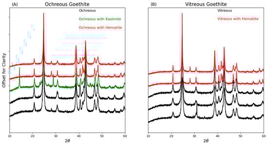
Figure 1.
XRD patterns for the 5 ochreous (A) and the 5 vitreous goethite samples (B) used in the study. Two of the ochreous samples in (B) were excluded due to occurrence of hematite, shown in red, and one due to the presence of kaolinite shown in green. Two of the vitreous samples in (B) were also excluded due to the presence of hematite (shown in red).
Four hematite samples were used to represent the initial hematite endmembers and consist of a synthetic hematite (Bayer 160), natural microplaty hematite and martite and a mixture of synthetic 95% hematite (Bayer 160) and 5% magnetite (Bayer 330). The latter sample is not used extensively in this study but is included to show the effect that magnetite can have on the formation of the boomerang and what might be expected if magnetite is present.
2.2. Additional Ochreous and Vitreous Preparation
The 2 ochreous and 3 vitreous samples were crushed and dry sieved to 6 different size fractions of +16 mm, +9.5 mm, +6.7 mm, +4.75 mm, +2 mm, and +1 mm and multiple spectral measurements across the varying particle sizes were collected. This increased the total number of spectral measurements available and allowed for natural spectral variability to be incorporated into the study.
2.3. Spectral Averaging
The reflectance spectra of each size fraction were collected with a pistol-grip 8° fore-optic mounted to an ASD VNIR/SWIR spectrometer. The pistol-grip was fixed above the samples to give a 7.5 cm measurement height. Each size fraction was placed into a tray and the surface levelled to minimise variation in sample height and measurements in a 5 × 3 grid collected (15 locations and spectral samples per size fraction). It is noted that surface leveling is not as effective for larger size fractions and the number of between-sample voids increases. The resulting spectra for a given size fraction were averaged using an equal weighting to obtain a single representative reflectance spectrum for each of the 6 size fractions. This yields a total of 12 ochreous endmember spectra and 18 vitreous endmember spectra. The resulting spot measurement from the mounted pistol-grip is approximately 1 cm and is comparable to the HyLoggerTM spot sample size (approximately 8 mm) used in the collection of the Hamersley Province diamond drillcore samples.
The resulting spectral endmembers are shown in Figure 2A for hematite, Figure 2B for ochreous goethite, and Figure 2C for vitreous goethite. The scatterplot of FWHM versus continuum hull corrected Fe Oxide wavelength is approximately linear as shown by the blue line in Figure 2D. The samples are coloured according to their composition while the averages of the goethite samples are shown with black dots.
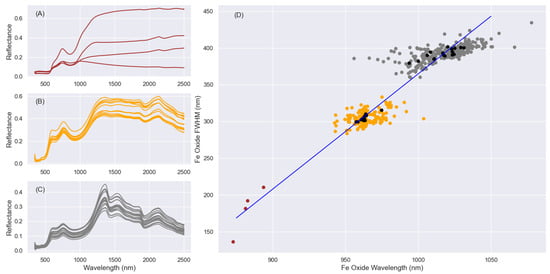
Figure 2.
The spectral endmembers and their locations when plotted as continuum hull corrected Fe Oxide Wavelength versus FWHM. (A–C) show the resulting spectral averages of the available endmembers across the 6 differing particle sizes (not highlighted). (A) 3 hematite endmembers and 1 magnetite+hematite endmember, (B) 12 average ochreous goethite endmembers, (C) 18 average vitreous goethite endmembers. (D) The continuum hull corrected Fe Oxide Wavelength and Fe Oxide FWHM values of the spectral endmembers prior to any averaging are shown and coloured as per (A–C) for type identification. The samples shown as black points are the ochreous and vitreous spectral average iron boomerang values, while the line is to simply highlight that the boomerang values of the endmembers are approximately linear.
2.4. Drillcore Data
The proposed regression model, still to be defined, was applied to 3 diamond drillcore from the Hamersley Province in Western Australia. A spectral mask was applied to ensure that any spectral core sample registering an absorption depth in the 2000 nm–2500 nm spectral region due to clays, micas, or carbonates was excluded. The spectra were collected with a HyLoggerTM with further processing carried out in Python. All 4 spectral metrics used are calculable by a user within the CSIRO developed The Spectral Geologist (TSG) software if required. It is noted that the definition of asymmetry within TSG is not the same as that used here but is still compatible.
3. Methods
The concept of the iron boomerang was introduced in [23] in a qualitative study as it applied to BIF hosted iron ore deposits. The generalised properties noted in that study are shown in Figure 3 (modified from [23]). Calculating the values of 2 spectral metrics, namely, the Fe Oxide Wavelength and the Fe Oxide FWHM, in drillcore data and plotting one against the other will produce plots resembling that of Figure 3. The study provided a qualitative assessment of the boomerang but did not expand on the quantification of the internal mechanisms behind the iron boomerang. Here the methods and workflow required to build a prediction model using a random forest regression (RFR) to predict relative mixing ratios of hematite, ochreous, and vitreous goethite is outlined. The choice of a RFR model trained on spectral metrics as opposed to other unmixing approaches [10,28,29,30] is discussed later.
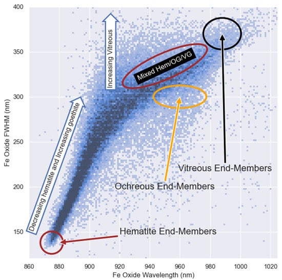
Figure 3.
A density plot showing the general composition and placement of key locations within the iron boomerang. At each end, and, if present, spectral endmembers of hematite and vitreous goethite can be found. Traversing the iron boomerang from left to right and bottom to top the proportion of hematite to goethite decreases toward a more goethite dominated region at wavelengths greater than approximately 920 nm. As the continuum hull corrected Fe Oxide FWHM increases within the goethite dominated region a move from more ochreous goethite to greater proportions of vitreous goethite is observed with ochreous goethite endmembers generally located in the orange circled region. Away from the endmembers are mixtures of hematite, ochreous and vitreous goethite.
3.1. Spectral Metrics
A total of 6 spectral metrics calculated from the 6A1→4T1 Fe3+crystal field absorption (CFA) centred around 900 nm, and an additional spectral metric defined between 1550 nm and 1850 nm is required. Table 2 summarises the spectral metrics, the wavelength region over which hull corrections are applied and an explanation of the metrics. Of the 7 calculated spectral metrics, 4 are input features to the RFR model. Prior to the calculation of any of spectral metrics a continuum hull correction is performed to remove the background effects and provide spectral normalisation.
Table 2.
The spectral metrics used in the formation of the iron boomerang and the subsequent mixing ratio modeling.
An example of a full range hull corrected spectrum, for illustrative purposes, is shown in Figure 4 and the key locations corresponding to the spectral metrics used and defined in Table 2. The point of maximum absorption of the 6A1→4T1 CFA is the Fe Oxide Depth which in turn informs the location of the Fe Oxide Wavelength and value of the Fe Oxide FWHM. The exact location of the Fe Oxide Wavelength can either be taken as the spectral band at the point of deepest absorption or a polynomial fit around the point of deepest absorption can be used for a more refined Fe Oxide estimate [11]. The wavelengths that intercept the hull corrected spectrum in a line perpendicular to the Fe Oxide Depth, and at the Fe Oxide Wavelength and labelled as λFWHML and λFWHMR are used to calculate the Fe Oxide asymmetry. Lastly, a continuum corrected maximum depth is calculated from the region in Figure 4 labelled as SWIR Drop-off and provides a means of gauging the potential vitreous goethite content.
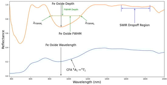
Figure 4.
The blue reflectance spectrum is a goethite sample showing the broad 6A1→4T1 crystal absorption feature. The upper spectrum in orange is a hull corrected spectrum. In this case the hull has been corrected across the full spectral range for illustrative purposes. The hull corrected 6A1→4T1 feature is used to define the point at which the deepest absorption value occurs and defines the Fe Oxide Wavelength, Fe Oxide FWHM, and Fe Oxide Depth spectral metrics. The wavelength region between 1550 nm and 1850 nm is the region where a local hull correction is performed, and the maximum depth recorded as the SWIR Drop-off metric.
Figure 5 shows 2 iron boomerang plots generated from spectral mixtures (discussed in the following section) of one of each of the hematite, ochreous, and vitreous endmembers in Figure 2. Figure 5A is coloured by the Fe Oxide asymmetry and Figure 5B by the SWIR Drop-off metric. Figure 5 represents the total of the 4 spectral metrics used as input features in the RFR model for the prediction of the relative hematite, ochreous, and vitreous goethite mixing ratios.
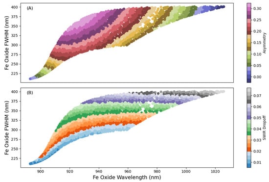
Figure 5.
The iron boomerang coloured by the 2 additional spectral parameters that are used in prediction modelling. (A) is coloured by the Fe Oxide Asymmetry where a value of 0 is symmetrical and 1 is right skewed. (B) is coloured by the SWIR drop-off between 1550 nm–1850 nm and increases as vitreous goethite increases. Refer to Figure 4 for how the 4 metrics are calculated.
3.2. Linear Mixing
In [23] and with reference to Figure 2 and Figure 4 the locations of the endmembers and their location within the iron boomerang suggested the outer edges of the boomerang are mixing pathways between the endmembers. To determine the viability of the suggestion, linear mixtures of the 3 endmembers of hematite, ochreous, and vitreous goethite were calculated. While linear or nonlinear mixing models could be used, we have opted to use linear mixing as early experimentation demonstrated that this approach was better suited to the problem. Known mixing ratios of the 3 endmembers were created, which in turn allow the calculation of the iron boomerang spectral metrics (see Table 2) and the subsequent plotting of the Fe Oxide Wavelength and Fe Oxide FWHM to ascertain the resulting mixing space, an example of which are seen in Figure 5.
The linear mixing model used is the pseudo absorbance rather than weighted endmember reflectance since the addition of absorbances in this regime is linear. The linearly mixed absorbance spectra are then back transformed into reflectance where any further spectral processing occurs. In the results section the expected errors in the mixing ratio are presented for both absorbance and reflectance mixing models. The pseudo absorbance is given by [31]:
where Rλ is the endmember spectral reflectance at wavelength λ. The calculation of the linear mixing [32] in absorbance space, and with wavelength dependencies not shown but implied, is given as,
where Wi is the fractional weighting of endmember Ai. Lastly, this is transformed back into reflectance space,
where Rmixed is the resulting linearly mixed spectrum. The spectral metrics outlined in Table 2 can be applied to the mixed spectra for plotting and training of an RFR model.
3.3. Random Forest Regression
A random forest regression [33,34,35] model is used for estimating the mixing ratios with the 4 previously defined spectral metrics used as input features. The choice of an RFR model as opposed to a direct spectral unmixing methodology [29,36,37] was made because it allows mixing ratio prediction without having to be overly concerned about the characteristics of the instrument providing the spectral samples. If an RFR model is utilised incorporating the spectral metrics previously outlined, then those same metrics can be calculated from a different instrument with different spectral band wavelength sampling and FWHM characteristics without the need for spectral resampling.
This scenario can occur when the RFR model is built on a benchtop, or laboratory-based spectrometer but the user wishes to infer the mixing ratios from samples collected or measured with a different spectrometer. The differences in the instruments would preferably be minimal as might be expected with hyperspectral instruments. However, inherent instrument differences can lead to differences in the calculated metrics. The results shown later in Section 4.3 discuss the effect of unknown spectral endmembers and demonstrate that the method itself is robust to variations that may occur in the spectral metrics.
In all cases the random forest regression models used are from the Python scikit-learn library [38], specifically the sklearn.ensemble.RandomForestRegressor library. The library implementation of the RFR has several hyperparameters that may be set if the user desires. In this study we only changed one hyperparameter from the default setting. The maximum tree depth was set at a value of 16 instead of the unbounded default. This was done after an initial assessment of the maximum tree depth on the final modelling error. Values greater than 16 did not yield any significant improvement and using a smaller maximum tree depth produces physically smaller RFR models. The number of estimators was left at the default of 100.
The input features to the RFR are the Fe Oxide Wavelength, FWHM, and Asymmetry and the SWIR Drop-off while the values trained against are the mixing ratios of the hematite, ochreous, and vitreous goethite endmembers. The mixed spectra were calculated at 5% intervals. Using the scikit-learn implementation allows for a multiple output so a single model for a given set of four features will infer all 3 mixing ratios simultaneously.
3.4. Workflow
The process for building a RFR model for inferring the relative hematite, ochreous and vitreous goethite mixing ratios is as follows:
- Define hematite, ochreous, and vitreous endmembers;
- Use Equations (1)–(3) with the endmembers of step 1 to generate spectral mixtures of known mixing ratios for the hematite, ochreous and vitreous endmembers;
- Calculate the spectral metrics in Table 2 for each spectrum in step 2; and
- Train the random forest regression model with a maximum tree depth of 16 with 100 estimators with the Fe Oxide Wavelength, FWHM, Asymmetry, and SWIR Drop calculated from step 3 as the input features and the known mixing ratios of hematite, ochreous, and vitreous goethite as the target values.
To infer the relative hematite, ochreous, and vitreous mixing ratios from a given spectral sample of unknown mixing ratios, one simply calculates the Fe Oxide Wavelength, FWHM, Asymmetry, and SWIR drop for that sample as outlined in Table 2 and runs the RFR model developed in step 4 in prediction mode using those 4 spectral metrics as the required input features.
It is noted that the term relative is used throughout the study. In VNIR/SWIR spectral data certain minerals do not have diagnostic features and cannot, therefore, be accounted for, or the spectra masked prior to prediction. Such minerals would include quartz, for example. If the system is simple enough and only contains hematite, ochreous, and vitreous goethite then the returned mixing ratios from SWIR masked spectra can represent absolute values.
4. Results
This section details results related to the characteristics of the iron boomerang and how its distinctive shape is formed via a linear mixing regime. It is demonstrated that linear mixing of the hematite, ochreous, and vitreous endmembers are the cause of the iron boomerang shape. This is followed by an accuracy assessment of the RFR model and lastly the application of RFR models using in-situ spectral endmembers to 3 Hamersley Province diamond drillcore.
4.1. Boomerang Shape and Linear Mixtures
There are a total of 864 spectral combinations of the library endmembers (4 × 12 × 18) which are multiplied by the total number of mixture weights used (444 mixture values in 5% increments). The bulk of the results shown do not include the 95% hematite−5% magnetite endmember as it is only used to show the effect of magnetite on the iron boomerang result for interest but is not used to infer the potential accuracy.
Shown in Figure 6 is the calculated Fe Oxide Wavelength versus Fe Oxide FWHM values for each of the 4 hematite endmembers linearly mixed with a single ochreous and vitreous endmember and coloured, except for the edges, by the ochreous goethite mixing ratio. In each case the distinct iron boomerang shape is produced and shows that its shape is explained by linear mixtures of hematite, ochreous, and vitreous goethite. The inset spectral plots show the endmembers used to generate the given iron boomerang. Figure 6A is the martite endmember, Figure 6B is the hematite (Bayer 160) endmember, Figure 6C is the premixed hematite−95%–magnetite−5% endmember and Figure 6D is the microplaty–hematite endmember.
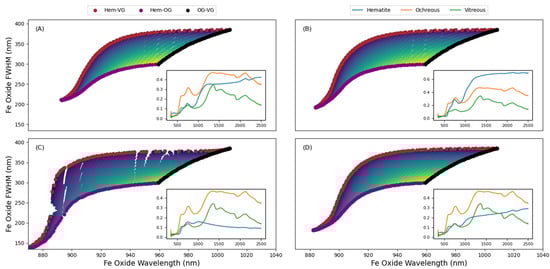
Figure 6.
The effect of the hematite endmember on the iron boomerang. Each plot is the iron boomerang manifold for the 3 spectral endmembers shown in the respective inset reflectance plot. The only variable in figures (A–D) is the hematite endmember. The upper-edge of the boomerang corresponding to a 2-mixture state of hematite and vitreous goethite (Hem-VG) while the lower-edge is a 2-mixture state of hematite and ochreous goethite (Hem-OG). The interior of the boomerang are 3-mixture states of the hematite, ochreous, and vitreous endmembers and are coloured by the percentage of vitreous goethite in the mixture. Note the void in (C) around an Fe Oxide Wavelength of 970 nm and Fe Oxide FWHM of 370 nm is a product of the linear mixing. The hematite endmembers are (A) martite, (B) hematite (Bayer 160), (C) hematite−95%–magnetite−5%, and (D) microplaty–hematite.
In each of the plots of Figure 6 the edges are given a single colour to highlight those mixtures which are due to 2-part linear mixtures of either hematite–ochreous goethite (Hem-OG, lower purple edge) or hematite–vitreous goethite (Hem-VG, upper brown edge) or ochreous–vitreous goethite (OG-VG, right-hand black edge), while the interior of each boomerang are mixtures of all 3 endmembers where the mixing ration of any given endmember is greater than 0. The internal colouring in this case is the ochreous goethite percentage in each mixture with bright colours representing increasing proportion of ochreous goethite and dark colours decreasing proportions.
Figure 6C, the hematite−95%–magnetite−5% endmember shows the effect that magnetite can have on the boomerang shape. Voids are noted along the top edge (2-part linear mixture) and is distinctly different from Figure 6A–C but is explained by examining the resulting spectrum generated in the 2-part linear mixture between the hematite endmember beyond 1000 nm and the vitreous endmember as described in the following section.
4.1.1. Hematite and Vitreous Linear Mixtures
Figure 7 shows the linear mixtures between the 4 hematite endmembers and all 18 vitreous goethite endmembers but coloured by the hematite endmember. The 18 vitreous goethite endmembers do not show large variational changes to the leading edge but are primarily driven by the hematite endmember as noted earlier. In Figure 7A the inset plot shows the 4 hematite endmembers (0) martite, (1) hematite (Bayer 160), (2) hematite−95%–magnetite−5%, and (3) microplaty–hematite. The deviation of the magnetite effected endmember is most distinct and is explained by considering Figure 7B. In Figure 7B the resulting hull corrected spectrum of the magnetite endmember and a vitreous goethite endmember in the 740–1360 nm spectral region is shown as a function of the hematite mixing ratio. As the proportion of vitreous goethite decreases the resulting linearly mixed absorption feature develops an observable 2 feature absorption and, in this case, causes the Fe Oxide Wavelength, as determined by the Fe Oxide Depth to abruptly shift from shorter wavelengths to longer wavelengths leading to the voids observed in Figure 6C.
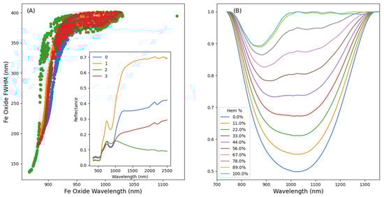
Figure 7.
(A) The distribution of the 2-mixture models for the 4 hematite endmembers (inset spectral plot) mixed with the 18 vitreous endmembers. The 4 hematite endmembers are (0) martite, (1) hematite (Bayer 160), (2) hematite−95%–magnetite−5%, and (3) microplaty–hematite. (B) The hull corrected linear mixtures of the hematite−95%-magnetite−5% endmember (see inset spectral plot) and a randomly selected vitreous endmember to show how the Hem-VG mixing gaps in (A) are manifested. The hematite endmember induces a leap from shorter wavelengths to longer wavelengths once the vitreous goethite reaches a high enough proportion (approximately 70% in this example). This is, generally, confined to those hematite’s that have a large drop-off from approximately +1000 nm.
4.1.2. Hematite and Ochreous Linear Mixtures
Figure 8 shows the results of making linear mixtures of hematite and ochreous–goethite only. Again, the inset plot shows the 4 hematite endmembers of (0) martite, (1) hematite (Bayer 160), (2) hematite−95%–magnetite−5%, and (3) microplaty–hematite. In this case the magnetite–ochreous produces a long-tailed edge that is distinct in appearance as compared to the other 3 hematite endmembers. As with the hematite–vitreous mixtures in Figure 7, the 2-endmember mixtures shown in Figure 8 are between the individual hematite endmembers and all 12 ochreous endmembers and coloured by the hematite endmember used to create the mixtures.
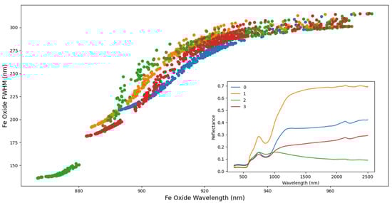
Figure 8.
The distribution of the 2-mixture models for the 4 hematite endmembers (inset spectral plot) mixed with the 12 ochreous endmembers. The 4 hematite endmembers are (0) martite, (1) hematite (Bayer 160), (2) hematite−95%–magnetite−5%, and (3) microplaty–hematite. The hematite−95%–magnetite−5% endmember (see inset spectral plot) has a distinct distribution but unlike mixtures with vitreous–goethite is essentially continuous.
4.2. Known Endmembers
To assess the potential accuracy of the proposed random forest model, based on Fe Oxide features extracted from linear mixtures of hematite, ochreous and vitreous endmembers, several random forest model configurations were tested. The first is the best-case scenario, while the second is a leave-one-out scenarios. In the best-case scenario, the assumption is that the entire set of potential endmembers are known a-priori and, hence, the input features to the random forest model cover all possible mixing scenarios. To assess the accuracy in this scenario the model was run in a repeated K-fold scenario comprised of 4 folds and repeated 5 times where each repeat selects 5 different folds than those previously used. This is the equivalent of holding out 25% of the input features and mixing ratios in each fold and training with the remaining 75%. After each K-fold the root-mean-square-error (RMSE) between the held out mixing ratios and the predicted mixing ratios (based on the held-out features) is calculated.
Table 3 summarises the results for the best-case scenario and is considered as the baseline accuracy. We do not show the results of each of the fold and repeat runs as they are extremely repetitive and are well summarised by a final average RMSE and the standard deviation of all calculated 20 RMSE values. In general, an approximate 4% modelling error is found for each of the three endmembers.
Table 3.
The average RMSE modeling error and standard deviations for a repeated K-fold scenario comprised of 4 folds and 5 repeats where each repeat selects 5 different folds than those previously used. This is the equivalent of holding out 25% of the input features and mixing ratios in each fold and training with the remaining 75%.
4.3. Unknown Endmembers
To assess the model when unknown endmembers are present and unaccounted for, in this case limited to unknown hematite endmembers as the effect of unknown ochreous and vitreous is minimal as shown earlier, several leave-one-out scenarios are run. In these cases, a RFR model was built with either one or two of the three possible hematite endmembers and the mixture of either one or two remaining hematite endmembers with the ochreous and vitreous endmembers was used to make a prediction and the RMSE calculated.
Table 4 shows the results of this analysis. The first column shows the hematite used to build the RFR model while the last column shows the hematite/s used to calculate the test 3-way mixtures of hematite, ochreous, and vitreous goethite, and input into the RFR model for prediction. So, in the first row of Table 4 the model is built using the martite–hematite endmember, while linear mixtures of the same ochreous and vitreous goethite with the hematite (Bayer 160) endmember were used to generate the required RFR feature inputs for the model to assess accuracy when the unknown hematite (Bayer 160) endmember is used. The respective hematite, ochreous, and vitreous columns show the calculated RMSE between the actual mixing ratios and the model prediction mixing ratios. The RMSE values in the hematite, ochreous, and vitreous columns are given in an X/Y format. The second value is the RMSE if a traditional linear mixing method is used, namely mixtures calculated with the reflectance rather than the pseudo absorbance.
Table 4.
The RMSE and standard deviation from 13 leave-one-or-many-out scenarios. The endmember exclusions are for hematite only. Column 1 is the hematite endmember, or members, used to train the model and column 5 is the hematite endmember, or endmembers, used to assess the model against. Columns 2–4 are the RMSE values for a given scenario with the RMSE values in the hematite, ochreous and vitreous columns in an X/Y format. The second value is the RMSE if a traditional linear mixing method is used, namely, mixtures calculated with the reflectance rather than the pseudo absorbance.
In general, improvements in the RMSE are noted when the pseudo absorbance is used for the mixing regime rather than the traditional reflectance mixing. The ochreous goethite estimations are affected the most by unknown hematite endmember knowledge (13% ± 6%). This can be explained by reference to Figure 8 and Figure 9, and the mixing paths of the martite, hematite (Bayer 160), and microplaty hematite endmembers. The latter 2 endmembers produce similar mixing paths while the martite endmember occupies a visibly different mixing path and can, depending on what endmember/s were used for modelling and testing, be quite removed from the true mixing path. It is noted that while the values in Table 4 are the RMSE for all potential mixture values (0–100%) the largest individual errors in predicted mixing ratio will generally occur in the mid-levels (30–60%) rather than where a given ratio is very large or very small.
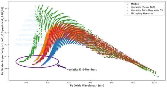
Figure 9.
The Fe Oxide Wavelength versus the Asymmetry for the 4 different hematite endmembers mixed with the same randomly selected ochreous and vitreous endmember. Circled in purple are those values for which the hematite mixing ratio terminates at 100%. It is apparent that hematite endmembers can be extracted by taking a representative selection across the terminating line circled.
The results in Table 4 represent the potential accuracy of the model in cases where a standard model might be used with no consideration of the actual hematite endmembers such that all potential endmembers may not be represented in the model. The last row of Table 4 shows the average RMSE and standard deviation of the estimated mixing ratios for a given endmember and are found to be approximately 14% ± 3% when the models are created using linear mixtures of reflectance spectra as opposed to 10% ± 4% when a pseudo absorbance linear mixing method is used.
Hematite Endmembers
Figure 9 shows the Fe Oxide Wavelength versus the Asymmetry for the 4 different hematite endmembers mixed with the same randomly selected ochreous and vitreous endmembers. Circled in Figure 9 are those values where the hematite mixing ratio terminates at 100%. What is apparent here is the hematite endmembers can be extracted by taking a representative selection across the terminating line circled in Figure 9. Applying this to measured drillcore which the various spectral indices have been calculated and manually selecting an evenly spaced selection from this same line allows the extraction of a dataset’s hematite endmembers and a means by which to reduce the overall RMSE.
The result of using this approach to define the hematite endmember/s and their impact on the mixing model is shown in Figure 10. Here the hematite endmembers are manually selected and combined with ochreous and vitreous endmembers to produce a new distribution from which to build a random forest regressor model. In Figure 10 the measured boomerang distribution is shown in blue while the base model distributions sit behind and are shown in an RGB scheme for hematite (brown), ochreous (orange), and vitreous goethite (black).
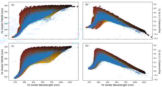
Figure 10.
The measured iron boomerang distribution is shown in blue while the base model distributions sit behind and are shown in an RGB scheme for hematite (brown), ochreous (orange), and vitreous goethite (black). (A,B) show the mixing space generated from the library endmembers of hematite, ochreous and vitreous goethite. (A) is the iron boomerang while (B) is the Fe Oxide Wavelength versus the Fe Oxide Asymmetry. Selecting in-situ hematite and ochreous endmembers, the vitreous is supplied from the library, leads to (C,D), respectively.
In Figure 10A,B the total mixing space when using the library endmembers only is shown with the familiar iron boomerang in Figure 10A and the Fe Oxide Wavelength versus the Fe Oxide Asymmetry in Figure 10B. With reference to Figure 10B the location of the hematite endmembers is obvious and allows data specific hematite endmembers to be selected. Additionally, and for further illustrative purposes, the ochreous endmembers used in Figure 10A,B can also be finetuned and selected from the measured data. The vitreous endmembers have not been reselected.
The impact of selecting dataset specific endmembers is shown in Figure 10C,D. The measured data in blue are, for the most part, encompassed by the new mixing space. The number of data points that fall outside of the mixing space are minor. As previously noted, using a model based on the actual endmembers is expected to lower the uncertainty on the inferred mixing ratios from approximately 10% to approximately 4–5%. It is important to note that the modelled distribution is not expected to take on the exact same shape as the measured data distribution since the range of all possible mixing ratios will, generally, occupy a larger mixing space than the measured boomerang.
4.4. Application to HyLogged Drillcores
In the presence of unknown hematite endmembers, the accuracy of the random forest regression can degrade by a factor of 2. This may be an acceptable level of accuracy, but it is preferable to make a model using endmembers sourced from the drillcore datasets themselves, if possible, to increase the accuracy of the regression. In this section the endmembers are sourced, where possible, from the drillcore spectral data themselves. This task is performed manually at this stage but is marked for automation in the future.
For each of the 3 drillcore two figures are shown. The first is a false colour image of the downhole estimated mixing ratios of hematite, ochreous, and vitreous goethite where the RGB values are determined from the relevant endmember mixing ratio. In this case the red channel is brown (hematite), the green channel is orange (ochreous goethite), and the blue channel is black (vitreous goethite). Alongside the down hole false colour image are the individual mixing proportions averaged over 1 m, which are followed by the core tray at 3 different depths down the core. The location of the core trays on the far right-hand column are shown in the mixing ratio columns and are coloured according to the depth ranges given in the core tray images.
The second is a 4-way subplot showing the iron boomerang for the drillcore coloured in the same manner and shows the individual spectral endmembers, coloured according to type, either selected from the drillcore or from the previously defined spectral library. The use of endmembers defined from the data itself or from the library is clarified in those individual results. It is noted that the sum of the mixing ratios in all the models for a given spectral sample is one. A summary of the overall modelling error is given in Table 5 along with the R2 value for each of the endmember types. The RMSE values in Table 5 assume that endmembers selected are representative of the dataset. However, in cases where an in-situ endmember cannot be reliably established the library endmembers are used and so the true RMSE is most likely around 10%.
Table 5.
The RMSE modeling error and R2 for each of the drillcore in question when 20% of the RFR input features and known mixing ratios are held out for testing.
4.4.1. Drillcore 1
Drillcore 1 is primarily comprised of hematite and ochreous goethite with less than 20% of vitreous goethite (Figure 11). The false colour image of Figure 11 does reveal subtle differences down hole and when combined with the mixing ratio plots allows us to define some potential domains within the drillcore. The elevated hematite and vitreous goethite from approximately 0 m–25 m are indicative of the so-called hardcap (highly weathered) zone. From 12 m to approximately 50 m the hematite content decreases while ochreous goethite increases into a hydrated zone. From approximately 100 m on the ochreous and hematite content would suggest the primary ore zone while the very last portion of the hole has hard martite with magnetite but noted as a rapid increase in “vitreous content” is indicative of a BIF.
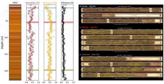
Figure 11.
The first column is a false colour image of the downhole estimated mixing ratios where the RGB values are determined from the relevant endmember mixing ratio and are colored as per the mixing ratio columns (columns 2–4) of hematite (brown), ochreous goethite (orange), and vitreous goethite (black). In columns 2–4 the mixing ratios are averaged over 1 m for the drillcore and coloured by their respective endmember colours. Column 5 shows colour images of the trays at specific locations in the drill core that show the range of ochreous and vitreous goethite and hematite. The depths the core trays span are shown in colored text above each tray with their locations corresponding to the coloured horizontal bar in columns 2–4.
Figure 12B–D show the endmembers used for drillcore 1. In this case the hematite and ochreous endmembers are selected from the dataset while the vitreous endmembers were supplied via the endmember library. The lack of vitreous in this case is evident when the upper edge where hematite and vitreous mixtures occur is examined and, hence, the choice of library endmember. The boomerang itself shows a drillcore dominated primarily by hematite and ochreous goethite.
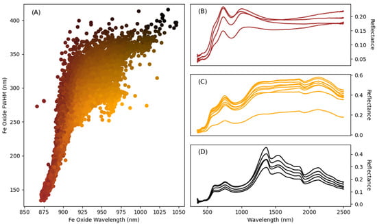
Figure 12.
(A) The false colour iron boomerang for drillcore 1 coloured in the same manner as the downhole plots, (B) in-situ selected hematite endmembers, (C) in-situ selected ochreous goethite endmembers, and (D) library selected vitreous goethite endmembers.
4.4.2. Drillcore 2
Drillcore 2 is approximately 60 m in depth. In Figure 13 the hematite content is found to be suppressed and the ochreous and vitreous goethite dominant. In Tray A (13.3 to 15.7 m) the elevated ochreous and vitreous goethite content and the low hematite content correspond to channel iron deposits (CID) sample overlying a soft hematite–goethite section (Tray B 35 m–37.2 m). In Tray C (52.1 m–54.9 m), the increase in vitreous goethite together with hardness is indicative of the hardcap zone. This finding is backed up by an examination of the iron boomerang in Figure 14A, which shows very little in hematite in the left-hand zone of the iron boomerang. The endmembers used for drillcore 2 are entirely composed of library endmembers. In this case the distribution of the data in the iron boomerang did not have enough points in those areas where the endmembers are known to reside. Hence the use of library endmembers.
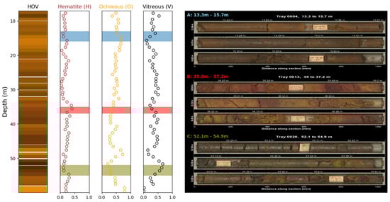
Figure 13.
The first column is a false colour image of the downhole estimated mixing ratios where the RGB values are determined from the relevant endmember mixing ratio and are colored as per the mixing ratio columns (columns 2–4) of hematite (brown), ochreous goethite (orange), and vitreous goethite (black). In columns 2–4 the mixing ratios are averaged over 1 m for the drillcore and coloured by their respective endmember colours. Column 5 shows colour images of the trays at specific locations in the drill core that show the range of ochreous and vitreous goethite and hematite. The depths the core trays span are shown in colored text above each tray with their locations corresponding to the coloured horizontal bar in columns 2–4.
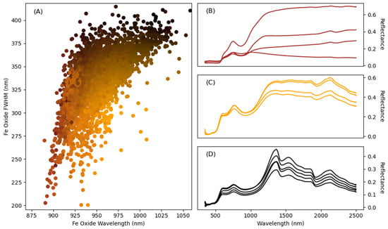
Figure 14.
(A) The false colour iron boomerang for drillcore 2 coloured in the same manner as the downhole plots, (B) library selected hematite endmembers, (C) library selected ochreous goethite endmembers, and (D) library selected vitreous goethite endmembers.
4.4.3. Drillcore 3
Drillcore 3 is 45 m thick with a clear 8 m zone of hematite noted at the top of the core corresponding to the dehydrated zone (Figure 15). The ochreous goethite between 8 m–40 m is generally constant around 25–30% while vitreous goethite dominates the rest of the core to approximately 40 m depth. This zone corresponds to the hardcap/hydrated zone. Tray C (39.71 m–43.2 m) corresponds to the ore zone with a higher amount of friable hematite and ochreous goethite and no vitreous goethite.
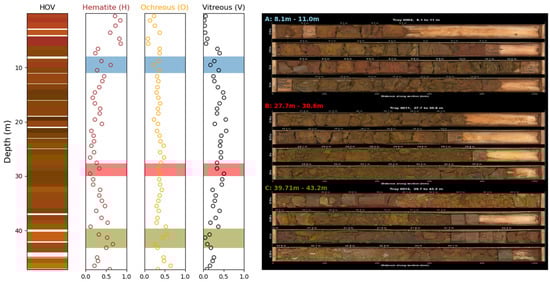
Figure 15.
Application of the boomerang methodology to drillcore 3. The first column is a false colour image of the downhole estimated mixing ratios where the RGB values are determined from the relevant endmember mixing ratio and are colored as per the mixing ratio columns (columns 2–4) of hematite (brown), ochreous goethite (orange), and vitreous goethite (black). In columns 2–4 the mixing ratios are averaged over 1 m for the drillcore and coloured by their respective endmember colours. Column 5 shows colour images of the trays at specific locations in the drill core that show the range of ochreous and vitreous goethite and hematite. The depths the core trays span are shown in colored text above each tray with their locations corresponding to the coloured horizontal bar in columns 2–4.
Figure 16 shows the calculated iron boomerang for drillcore 3 and the various endmembers used to form the RFR model in Figure 16B–D. In this case the library endmembers were used for the ochreous goethite and in-situ endmembers for the hematite and vitreous goethite.
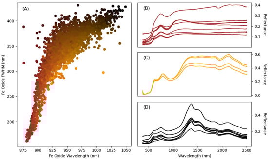
Figure 16.
(A) The false colour iron boomerang for drillcore 3 coloured in the same manner as the downhole plots, (B) in-situ selected hematite endmembers, (C) library selected ochreous goethite endmembers, and (D) in-situ selected vitreous goethite endmembers.
5. Discussion
The work presented herein demonstrated that the distinct shape formed by the scatter plot of the Fe Oxide Wavelength and FWHM of the 6A1→4T1 Fe 3+ CFA is the product of linear mixing of 3 iron oxides and oxy-hydroxides endmembers of hematite, ochreous, and vitreous goethite. Secondly, it was shown that the distribution of the additional spectral metrics, such as the Fe Oxide Asymmetry and the SWIR Drop-off, used to describe the iron boomerang are also well distributed. This, in turn, was used to define an input feature set which can be used to train a random forest regression model for the prediction of the relative hematite, ochreous, and vitreous goethite mixing proportions.
While it was shown that the complete knowledge of the endmembers in a dataset enables extremely good accuracy to be attained, on the order of 5% RMSE for all 3 iron-bearing mineral types, a lack of representative hematite endmembers in the regression model will elevate the RMSE to approximately 10%. However, by combining the Fe Oxide Wavelength and Asymmetry into a scatter plot a means selecting the appropriate hematite endmembers is found.
The results of applying the methodology to 3 diamond drillcore from the Hamersley Province in Western Australia demonstrated that downhole domains are identifiable. The benefits of applying the proposed methodology are better ore zone delineation, hardcap and hydrated zone identification, the potential for more accurate resource modeling, and identification of potential problematic zones. If the outputs from the model are combined into domaining or changepoint detection algorithms it would be expected that the boundaries of the domains could be defined in an automated fashion.
6. Conclusions
This value of this work to estimate mixing ratios or proportions of hematite, ochreous, and vitreous goethite was established and shows that previous work that focused on hematite–goethite distinction only, or ochreous–vitreous goethite only can be represented in a singular simple method. This work combined with spectral metrics related to the 6A1→4T1 Fe3+ CFA demonstrated that the averaged spectral response of iron ores are inherently a product of linear spectral mixing. The novel aspect here is that the mixtures of library endmembers can be defined by those spectral metrics rather than having to enact a traditional spectral unmixing methodology.
The use of such spectral metrics combined with the known mixing ratios and a random forest regressor is advantageous in scenarios where multiple spectral sensors might be used to gather spectral samples. While the field of linear spectral unmixing is well established many of the techniques assume that the spectral data are produced by a singular instrument. In locations with sufficient spectral data volume and where the spectral endmembers can be defined a regression model can be trained. This provides a means of using spectral measurements from handheld field spectrometers to calculate the boomerang metrics required for input to the regression model. In turn, the mixing ratios or proportions of hematite, ochreous, and vitreous goethite can be inferred without having to directly resample the spectra to other instrument wavelength specifications. This implies that both instruments are hyperspectral. At its most basic the iron boomerang allows a visual comparison of differing datasets collected from different instruments.
Further work will include a more detailed analysis of bedded iron deposits (BID) drillcores with known and well-defined domains and an assessment of routines for the automatic selection of spectral endmembers within the data. Additionally, this study did not address the issue of compounding minerals, such as kaolinite and carbonate, and will seek to incorporate that into future work. In samples containing additional minerals the wavelengths and FWHM values may be shifted, and such cases may require the addition of endmembers that represent them to avoid under or overestimation of the hematite, ochreous and vitreous goethite proportions.
Author Contributions
Conceptualization, A.R. and E.R.; methodology, A.R.; software, A.R.; validation, A.R. and E.R.; formal analysis, A.R. and E.R.; writing—original draft preparation, A.R.; writing—review and editing, A.R. and E.R.; visualization, A.R. All authors have read and agreed to the published version of the manuscript.
Funding
This work was funded as part of Minerals Research Institute of Western Australia (MRIWA) project 557.
Acknowledgments
The authors would like to acknowledge the following for their support: BHP Iron Ore, Bureau Veritas, CSIRO Mineral Resources, FMGL, MRIWA, Rio Tinto Iron Ore, and Roy Hill.
Conflicts of Interest
The authors declare no conflict of interest.
References
- Cudahy, T.J.; Ramanaidou, E.R. Measurement of the hematite: Goethite ratio using field visible and near-infrared reflectance spectrometry in channel iron deposits, Western Australia. Aust. J. Earth Sci. 1997, 44, 411–420. [Google Scholar] [CrossRef]
- Haest, M.; Cudahy, T.; Laukamp, C.; Gregory, S. Quantitative mineralogy from infrared spectroscopic data. I. Validation of mineral abundance and composition scripts at the Rocklea Channel iron deposit in Western Australia. Econ. Geol. 2012, 107, 209–228. [Google Scholar] [CrossRef]
- Haest, M.; Cudahy, T.; Laukamp, C.; Gregory, S. Quantitative mineralogy from infrared spectroscopic data. II. Three-dimensional mineralogical characterization of the Rocklea Channel iron deposit, Western Australia. Econ. Geol. 2012, 107, 229–249. [Google Scholar] [CrossRef]
- Ramanaidou, E.R.; Wells, M.A. hyperspectral imaging of iron ores. In Proceedings of the 10th International Congress for Applied Mineralogy (ICAM), Trondheim, Norway, 1–5 August 2011; Springer: Berlin/Heidelberg, Germany, 2012; pp. 575–580. [Google Scholar]
- Cudahy, T.; Jones, M.; Thomas, M.; Laukamp, C.; Caccetta, M.; Hewson, R.; Verrall, M.; Hacket, A.; Rodger, A. Mineral Mapping Queensland: Iron Oxide Copper Gold (IOCG) Mineral System Case History, Starra, Mount Isa Inlier; Australasian Institute of Mining and Metallurgy: Gold Coast, QLD, Australia, 2008; pp. 153–160. [Google Scholar]
- Ramanaidou, E.; Morris, R.C. A synopsis of the channel iron deposits of the Hamersley Province, Western Australia. Appl. Earth Sci. 2010, 119, 56–59. [Google Scholar] [CrossRef]
- Ramanaidou, E.R.; Schodlok, M. Hyperspectral mapping of bif and iron ores. In Proceedings of the AGU Fall Meeting, San Francisco, CA, USA, 3–7 December 2012; Volume 2012, p. NS23A-1630. [Google Scholar]
- Duuring, P.; Laukamp, C. Mapping Iron Ore Alteration Patterns in Banded Iron-Formation Using Hyperspectral Data: Beebyn Deposit, Pilbara Craton, Western Australia; Geological Survey of Western Australia: East Perth, Australia, 2016. [Google Scholar]
- Murphy, R.J.; Monteiro, S. Mapping the distribution of ferric iron minerals on a vertical mine face using derivative analysis of hyperspectral imagery (430–970 nm). ISPRS J. Photogramm. Remote Sens. 2013, 75, 29–39. [Google Scholar] [CrossRef]
- Magendran, T.; Sanjeevi, S. Hyperion image analysis and linear spectral unmixing to evaluate the grades of iron ores in parts of Noamundi, Eastern India. Int. J. Appl. Earth Obs. Geoinf. 2014, 26, 413–426. [Google Scholar] [CrossRef]
- Rodger, A.; Laukamp, C.; Haest, M.; Cudahy, T. A simple quadratic method of absorption feature wavelength estimation in continuum removed spectra. Remote Sens. Environ. 2012, 118, 273–283. [Google Scholar] [CrossRef]
- Laukamp, C.; Termin, K.A.; Pejcic, B.; Haest, M.; Cudahy, T. Vibrational spectroscopy of calcic amphiboles—Applications for exploration and mining. Eur. J. Miner. 2012, 24, 863–878. [Google Scholar] [CrossRef]
- Rodger, A.; Fabris, A.; Laukamp, C. Feature extraction and clustering of hyperspectral drill core measurements to assess potential lithological and alteration boundaries. Minerals 2021, 11, 136. [Google Scholar] [CrossRef]
- Laukamp, C.; Rodger, A.; LeGras, M.; Lampinen, H.; Lau, I.; Pejcic, B.; Stromberg, J.; Francis, N.; Ramanaidou, E. Mineral physicochemistry underlying feature-based extraction of mineral abundance and composition from shortwave, mid and thermal infrared reflectance spectra. Minerals 2021, 11, 347. [Google Scholar] [CrossRef]
- Kämpf, N.; Schwertmann, U. Goethite and hematite in a climosequence in southern Brazil and their application in classification of kaolinitic soils. Geoderma 1983, 29, 27–39. [Google Scholar] [CrossRef]
- Madeira, J.; Bedidi, A.; Cervelle, B.; Pouget, M.; Flay, N. Visible spectrometric indices of hematite (Hm) and goethite (Gt) content in lateritic soils: The application of a Thematic Mapper (TM) image for soil-mapping in Brasilia, Brazil. Int. J. Remote Sens. 1997, 18, 2835–2852. [Google Scholar] [CrossRef]
- Ramanaidou, E.; Wells, M.; Lau, I.; Laukamp, C. Characterization of iron ore by visible and infrared reflectance and, Raman spectroscopies. In Iron Ore; Elsevier: Amsterdam, The Netherlands, 2015; pp. 191–228. [Google Scholar] [CrossRef]
- Ramanaidou, E.R.; Wells, M.; Belton, D.X.; Verrall, M.; Ryan, C. Mineralogical and microchemical methods for the characterization of high-grade banded iron formation-derived iron ore. In Banded Iron Formation-Related High-Grade Iron Ore; Society of Economic Geologists: Littleton, CO, USA, 2008. [Google Scholar]
- Ramanaidou, E.; Wells, M.; Lau, I.; Laukamp, C. Chapter 6—Characterization of iron ore by visible and infrared reflectance and raman spectroscopies. In Iron Ore, 2nd ed.; Lu, L., Ed.; Woodhead Publishing Series in Metals and Surface Engineering; Woodhead Publishing: Cambridge, UK, 2022; pp. 209–246. ISBN 978-0-12-820226-5. [Google Scholar]
- Fonteneau, L.C.; Martini, B.; Elsenheimer, D. Hyperspectral imaging of sedimentary iron ores–beyond borders. ASEG Ext. Abstr. 2019, 2019, 1–5. [Google Scholar] [CrossRef] [Green Version]
- Clout, J.; Manuel, J. Mineralogical, chemical, and physical characteristics of iron ore. In Iron Ore; Elsevier: Amsterdam, The Netherlands, 2015; pp. 45–84. [Google Scholar] [CrossRef]
- Manuel, J.R.; Clout, J.M.F. Goethite classification, distribution and properties with reference to Australian iron deposits. Proc. Iron Ore 2017, 567–574. [Google Scholar]
- Rodger, A.; Ramanaidou, E.; Laukamp, C.; Lau, I. A qualitative examination of the iron boomerang and trends in spectral metrics across iron ore deposits in Western Australia. Appl. Sci. 2022, 12, 1547. [Google Scholar] [CrossRef]
- Huntington, J.; Whitbourn, L.; Mason, P.; Berman, M.; Schodlok, M.C. HyLogging—Voluminous industrial-scale reflectance spectroscopy of the earth’s subsurface. In Proceedings of the ASD and IEEE GRS Art, Science and Applications of Reflectance Spectroscopy Symposium, Boulder, CO, USA, 23–25 February 2010; Volume 2, p. 14. [Google Scholar]
- Smith, B.R.; Huntington, J.F. National Virtual Core Library NTGS Node: HyLogger 2–7; Northern Territory Geological Survey: Darwin, Australia, 2010. [Google Scholar]
- Cracknell, M.J.; Jansen, N.H. National virtual core library HyLogging data and Ni–Co laterites: A mineralogical model for resource exploration, extraction and remediation. Aust. J. Earth Sci. 2016, 63, 1053–1067. [Google Scholar] [CrossRef]
- Schodlok, M.C.; Whitbourn, L.; Huntington, J.; Mason, P.; Green, A.; Berman, M.; Coward, D.; Connor, P.; Wright, W.; Jolivet, M. HyLogger-3, a visible to shortwave and thermal infrared reflectance spectrometer system for drill core logging: Functional description. Aust. J. Earth Sci. 2016, 63, 929–940. [Google Scholar]
- Du, B.; Wang, S.; Wang, N.; Zhang, L.; Tao, D.; Zhang, L. Hyperspectral signal unmixing based on constrained non-negative matrix factorization approach. Neurocomputing 2016, 204, 153–161. [Google Scholar] [CrossRef]
- Bao, W.; Li, Q.; Xin, L.; Qu, K. Hyperspectral unmixing algorithm based on nonnegative matrix factorization. In Proceedings of the 2016 IEEE International Geoscience and Remote Sensing Symposium (IGARSS), Beijing, China, 10–15 July 2016; pp. 6982–6985. [Google Scholar]
- Gao, H.; Chen, L.; Li, C.; Zhou, H.; Zhang, S. A hyper-spectral unmixing method based on improved non-negative matrix factorization. J. Comput. Theor. Nanosci. 2016, 13, 8689–8694. [Google Scholar] [CrossRef]
- Rinnan, Å.; van den Berg, F.; Engelsen, S.B. Review of the most common pre-processing techniques for near-infrared spectra. TrAC Trends Anal. Chem. 2009, 28, 1201–1222. [Google Scholar] [CrossRef]
- Ducasse, E.; Adeline, K.; Briottet, X.; Hohmann, A.; Bourguignon, A.; Grandjean, G. Montmorillonite estimation in clay–quartz–calcite samples from laboratory SWIR imaging spectroscopy: A comparative study of spectral preprocessings and unmixing methods. Remote Sens. 2020, 12, 1723. [Google Scholar] [CrossRef]
- Breiman, L. Random forests. Mach. Learn. 2001, 45, 5–32. [Google Scholar] [CrossRef] [Green Version]
- McKay, G.; Harris, J.R. Comparison of the data-driven random forests model and a knowledge-driven method for mineral prospectivity mapping: A case study for gold deposits around the Huritz Group and Nueltin Suite, Nunavut, Canada. Nat. Resour. Res. 2016, 25, 125–143. [Google Scholar] [CrossRef]
- Kuhn, S.; Cracknell, M.J.; Reading, A.M. Lithologic mapping using Random Forests applied to geophysical and remote-sensing data: A demonstration study from the Eastern Goldfields of Australia. Geophysics 2018, 83, B183–B193. [Google Scholar] [CrossRef]
- Keshava, N. A survey of spectral unmixing algorithms. Linc. Lab. J. 2003, 14, 55–78. [Google Scholar]
- Keshava, N.; Mustard, J.F. Spectral unmixing. IEEE Signal Process. Mag. 2002, 19, 44–57. [Google Scholar] [CrossRef]
- Pedregosa, F.; Varoquaux, G.; Gramfort, A.; Michel, V.; Thirion, B.; Grisel, O.; Blondel, M.; Prettenhofer, P.; Weiss, R.; Dubourg, V. Scikit-learn: Machine learning in Python. J. Mach. Learn. Res. 2011, 12, 2825–2830. [Google Scholar]
Publisher’s Note: MDPI stays neutral with regard to jurisdictional claims in published maps and institutional affiliations. |
© 2022 by the authors. Licensee MDPI, Basel, Switzerland. This article is an open access article distributed under the terms and conditions of the Creative Commons Attribution (CC BY) license (https://creativecommons.org/licenses/by/4.0/).