Prediction of Sulfur Removal from Iron Concentrate Using Column Flotation Froth Features: Comparison of k-Means Clustering, Regression, Backpropagation Neural Network, and Convolutional Neural Network

Abstract

Froth feature extraction plays a significant role in the monitoring and control of the flotation process. Image-based soft sensors have received a great deal of interest in the flotation process due to their low-cost and non-intrusive properties. This study proposes data-driven soft sensor models based on froth images to predict the key performance indicators of the flotation process. The ability of multiple linear regression (MLR), the backpropagation neural network (BPNN), the k-means clustering algorithm, and the convolutional neural network (CNN) to predict the amount of sulfur removal from iron ore concentrate in the column flotation process was examined. A total of 99 experimental results were used to develop the predictive models. Extracted froth features including color, bubble shape and size, texture, stability, and velocity were used to train the traditional predictive models, whereas in the CNN model the froth images were directly fed into the model. The results comparison indicated that the three-layered feedforward NN model (17-10-1 topology) and CNN model provided better predictions than the MLR and k-means algorithm. The BPNN model displayed a correlation coefficient of 0.97 and a root mean square error of 4.84% between the actual data and network output for both training and the testing datasets. The error percentages of the CNN, BPNN, MLR and k-means models were 10, 11, 15 and 18%, respectively. This study can become a key technical support for the application of intelligent models in the control of the operational variables for the flotation process used to desulfurize iron concentrate.

1. Introduction

Flotation is a significant industrial technology for separating valuable minerals from tailings. It is a complicated physical-chemical separation method that takes advantage of differences in the surface properties of valuable and gangue minerals [1]. Due to the depletion of high-grade iron reserves and the need for very fine grinding to improve liberation, flotation is the most effective way to remove impurities from iron ore concentrate [2,3].

Although the flotation process has been widely used over a long period of time, how to evaluate the operational conditions, the automatic control and robust model of the process are challenging issues and still have not been fully considered by academic scholars. Furthermore, the weakness of sufficiently accurate and reliable process measurements amplifies this difficulty [4]. The ultimate goal in the flotation process is to maximize the separation between valuable minerals (concentrate) and gangue minerals (tailings) [5]. Technically, the performance of the flotation process is described by the concentrate characteristics (grade and recovery). These are important economic and technical indexes needed for process control and optimization [6]. Accurate values of these parameters are obtained only after sampling, filtration, drying, preparation and chemical analysis of samples, which are time-consuming operations [7]. In industrial plants, the grade can be continuously measured using an XRF analyzer and the recovery can only be calculated from a mass balancing [8,9]. The online measurement of these parameters with a relatively low accuracy using an X-ray analyzer generally requires the purchase and maintenance of costly and sophisticated equipment [5,10,11], which justifies the execution of models for the prediction of key performance indicators based on secondary variables.

Due to the nonlinear and complex nature of the flotation process, the large number of variables involved, and the very limited understanding of the physicochemical rules of the flotation process, accurate prediction of grade and recovery parameters is a difficult task [12,13,14,15]. Therefore, data-driven approaches requiring less prior knowledge about the system state variables (the input/output) are viewed as alternative strategies for modeling the flotation process. In the past few decades, modelling and predicting flotation behavior based on operational variables (such as reagent dosages) using numerical techniques has been extensively studied by researchers [16,17,18,19,20,21,22], although there is no universally accepted forecasting model. Most of these models only used relatively few operational parameters as the input variables so that they failed to enable the capture of the strong nonlinear relationship between the variables in a wide range of operating conditions. These models still have challenges, such as needing a large quantity of data, and have a complex configuration that limits their application.

In the last ten years, several studies have shown that the froth’s appearance contains a lot of valuable information, which plays a pivotal role in raising the flotation process efficiency [23]. The froth’s surface appearance reflects the changes in the flotation process induced by those affecting the operational variables, such as air flow rate and dosage of reagents [24]. Then, it can be directly used for flotation metallurgical performance estimation [25,26]. Traditionally, in the flotation plant the froth state is observed by experienced workers in order to control and make a decision for the working conditions [7]. However, decision-making based on the monitoring of froth surface changes just by the naked eye is inaccurate; that is, a time-consuming operation that limits the real-time control of the process. Therefore, the combination of froth imaging analysis techniques and the predictive mathematical models could provide the soft sensors for modelling the effects of operating variables on flotation process performance.

In recent years, there has been a rapid development in computing technology with an increased interest in machine vision applications for monitoring, analyzing and controlling the output of processes for most engineering purposes [27,28]. Machine vision is an automated, non-destructive and cost-effective alternative method used for the on-stream estimation of the efficiency of the flotation process. Image processing methods have been developed for the extraction and interpretation of froth appearance features such as color and texture [29,30,31,32], velocity [33,34], mineral loading rate [35], stability [11,36], and bubble size [25,37]. These studies showed that many methods can be used to extract and analyze the froth features; thus, several extracted features should be addressed at the same time for a better interpretation of froth behavior.

The performance of the reverse flotation of iron ores is largely governed by the interactions between the operational variables, which are complex. The prediction of the amount of sulfur removal in the reverse flotation of iron ore concentrate is an important issue to enhance the process efficiency. When the sulfur content of iron concentrate increases, the sulfur recovery and efficiency will reduce. In this situation, the operators at concentrators try to identify the problem and find a way to fix it based on the froth surface appearance. Visual assessments by operators are time-consuming and difficult tasks that can be carried out only at a given time. An image-based soft sensor with a view to monitor and control the operating conditions could be a great help for operators at flotation plants. Due to a dearth of reports on the properties of flotation froth during the desulfurization of iron concentrate [38], this research opted to combine the machine vision system and different statistical and intelligent techniques with a view to investigating the relationship between column flotation performance (sulfur recovery) and the froth features under different operating conditions.

For this, a dataset of images was first captured from froth surfaces at defined time intervals. Afterward, the bubble size and shape, froth color, texture and dynamic features (froth velocity and stability) were considered as good supplements for operating condition recognition prior to an offline extraction of the images from the desulfurization of iron ore concentrate using the in-column flotation. Finally, a comparative study was carried out using multiple linear regression (MLR), the k-means algorithm, the backpropagation neural network (BPNN) and the convolutional neural network (CNN) to predict the flotation performance based on froth features.

The machine learning models, such as NN, are widely used as a powerful approach for classification and prediction because of their non-linear learning ability. The NN is a computational method developed by copying human brain behavior. The NN is able to extract the complex nonlinear relationships existing between input and output variables through a highly interconnected system of simple processing elements (neurons or nodes) [39]. Recently, the models based on BPNN have been widely used as rapid and reliable tools for forecasting flotation performance [40,41]. Many studies in the literature specialized in the integration of machine vision and machine learning systems for improving the flotation process control. The proposed soft sensors were capable of extracting and analyzing the froth image features and using them as the inputs to the machine learning models [42,43].

MLR is another estimation tool which can help to predict the flotation performance based on a number of froth image features. The MLR model is presented based on fitting a linear equation to observed data. The main advantage of MLR is its simple form and easily interpretable mathematical expression [44]. The MLR is easy to formulate and has been used in flotation research to obtain models as an alternative to other mathematical methods [4,19].

The use of clustering algorithms has been widely used in diverse fields of study to offer a favorable alternative to traditional prediction methods [45,46]. Clustering is a process of organizing a set of objects into groups of similar objects, based on their characteristics. The k-means algorithm is one of the well-known unsupervised clustering techniques which is mainly applied in image and signal processing, pattern recognition and data mining [47]. K-means clustering is an iterative algorithm that tries to minimize variation within the clusters, and maximize variation between clusters [48,49]. In this research, the k-means algorithm is proposed to classify the froth characteristics to estimate the sulfur recovery in the column flotation process at different operating conditions.

The above-mentioned models concentrate on extracting specific froth features such as bubble size, color, and stability for classification of froth images to evaluate the flotation process performance. The big challenge of these models is that the prediction accuracy remarkably relies on the capability of feature extraction methods. Furthermore, these models are not sufficiently effective and reliable because they employ only low-level features without having enough mid-level and high-level features [50]. To overcome this problem and develop the classification accuracy, a deep learning method has been developed to classify image features under different conditions.

The convolutional neural network (CNN), one of the fastest-growing deep leaning algorithms, was developed for the classification of objects in the fields of engineering [51,52]. This method obviates the complexity of image modification and allows users to enter the original image directly to the model.

CNN was first implemented for froth image feature extraction in 2018 by Fu and Aldrich. They proved that the CNN model could generate more accurate results than the traditional models in the processing of flotation froth images. Recently, many researchers have employed CNN as a robust and efficient model for the evaluation of flotation influencing factors and the prediction of metallurgical performance parameters [5,53,54]. This article provides the application of CNN to categorize the collected froth images during the column flotation process. Then, its classification accuracy was compared to the traditional models.

Despite the fact that the above-mentioned methods were all individually used to forecast the mineral flotation performance, there is still a gap in identifying the best method with the highest prediction accuracy, especially the amount of sulfur removal from iron ore concentrate. Thus, the current study compared four methods of MLR, k-means, BPNN, and CNN to predict the amount of sulfur removal in the desulfurization of iron ore concentrate. The aim of this work was to elucidate if these predictive models could predict column flotation performance for the desulfurization of the iron ore concentrate with high accuracy based on the analysis of froth image characteristics. Such studies can make a remarkable contribution towards the improvement of soft sensors on the basis of froth image analysis for the real-time monitoring and control of flotation process.

In the following section, the reverse column flotation process of iron ore concentrate and the image-acquisition device are presented. Then, the techniques for extraction of froth features and the predictive models are briefly introduced. In the third part, the prediction results obtained by k-means, MLR, BPNN, and CNN methods are discussed. In the Section 4, the performances of these methods are compared.

2. Materials and Methods

2.1. Iron Ore Concentrate

The sample used in the present study was taken from the feed stream of the mechanical flotation cells in an iron ore concentrate plant in Iran. In this plant, the iron ore after comminution, gravity and magnetic separation, is fed to the flotation cells. The feed flotation has high sulfur (pyrite) content. In general, pyrite is considered as a gangue mineral creating problems during the steelmaking processes [55]. Sulfur causes brittleness and frangibility of steel at high temperatures, reduces weldability, increases corrosion, air pollution during the pellet-firing process, increases limestone consumption and slag production in the steelmaking procedure [56]. Pyrite and pyrrhotite are paramagnetic minerals and are attracted by the magnetic field in the vicinity of iron ores (magnetite and hematite). Therefore, they are not completely recovered by magnetic separators [57]. In this plant, the concentrate from the magnetic separation generally presents a sulfur content of 0.4 to 0.6%, which value surpasses the allowable limit for steel production (0.1%). The reverse flotation conducted at the end of the processing circuit enables a reduction of the sulfur content in the magnetic separation concentrate.

The representative flotation feed sample consisted of 63.3% Fe, 1.48% FeO with a significant sulfur content 0.50%. The particle size analysis of the representative sample 188 gave the d80 equal to 95 μm.

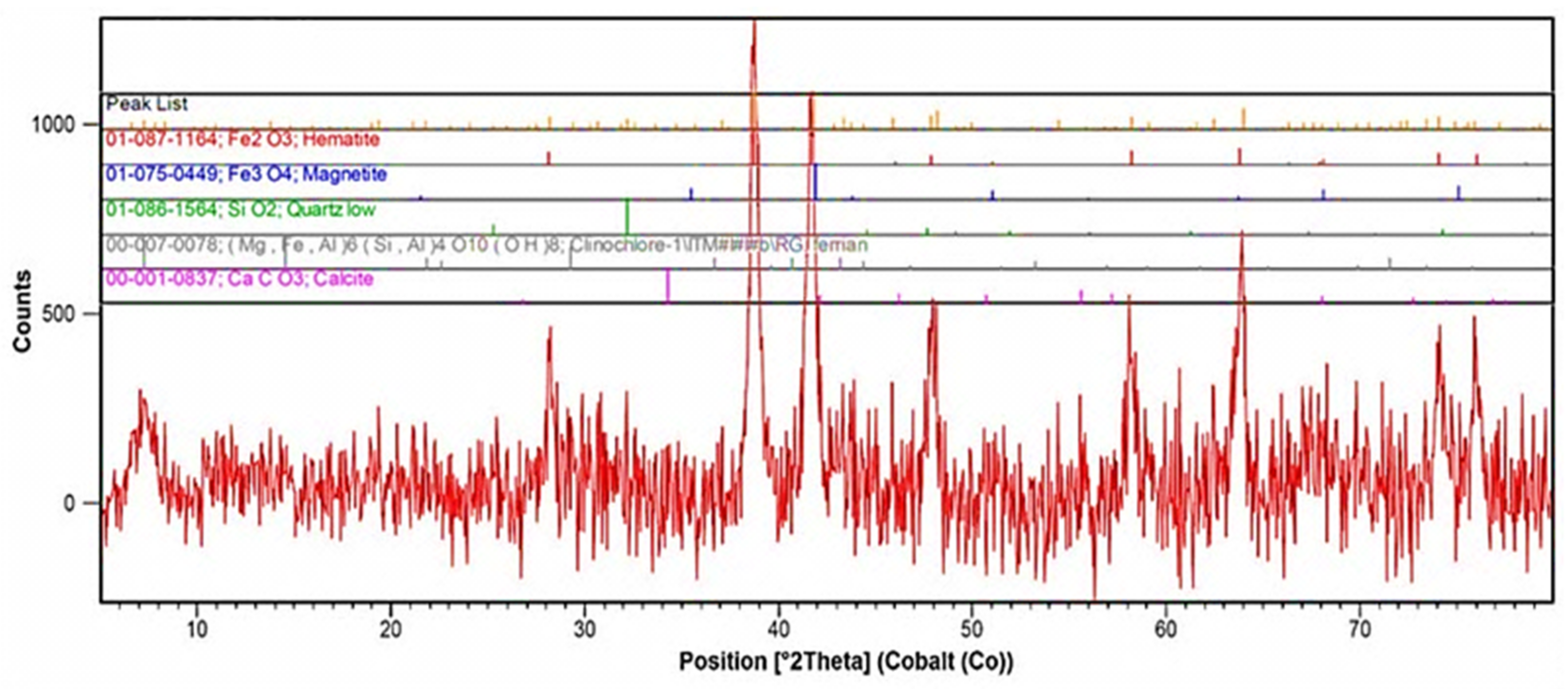
Mineralogical and liberation degree studies of the sample were conducted using optical microscope (Axio Plan 2, Zeiss, Germany) and wild zoom stereo microscope (Zeiss, Germany), respectively. The main iron minerals were hematite, magnetite and goethite. Calcite, quartz, dickite, chlorite and pyrite were the main gangue minerals. The results of X-ray diffraction pattern (XRD) analysis of the sample are shown in Figure 1. The XRD analysis confirmed the microscopic findings. Mineral liberation studies showed that more than 90% of pyrite particles were liberated at -105 μm.

2.2. Column Flotation Test

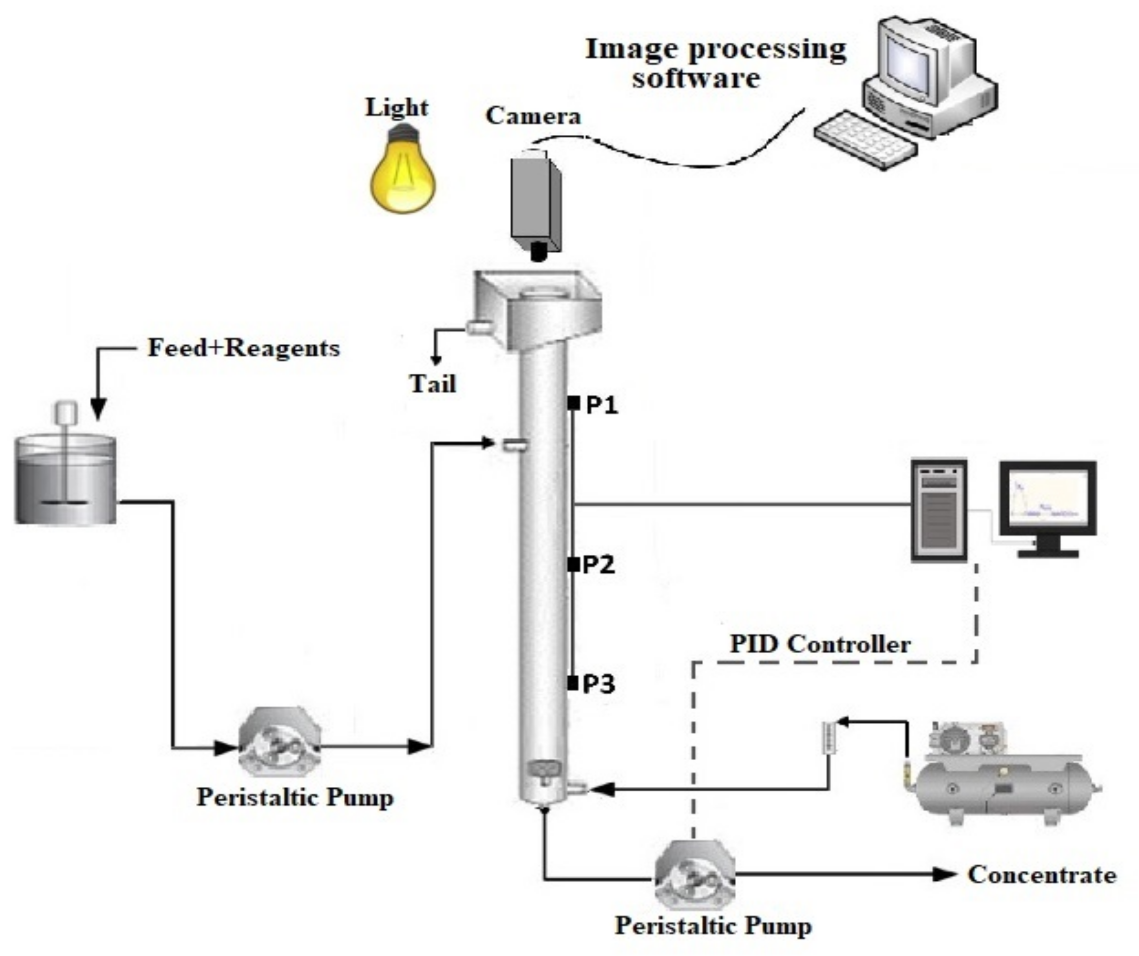
The tests were carried out in a plexiglass cell column of 400 cm in height, and 10 cm inside diameter in order to desulfurize the iron ore concentrate. To provide the initial feed, a tank equipped with a stirrer was used to prevent the material from settling while being prepared. Two peristaltic pumps were used: one for sending the feed to the middle of the cell and the other for withdrawing the pulp at the bottom of the cell. During the experiments, the pulp pH was continuously measured by a digital laboratory pH meter and adjusted to the desired value by adding sulfuric acid or NaOH.

Since the purpose of the in-column flotation operation was to reduce the sulfur content in the final product, potassium amyl xanthate (PAX) as a collector and MIBC as a frother were used. After adjusting the pH and sufficient mixing with chemical reagents (five minutes), the pulp was entered into the cell at a flow rate of 1.5–2 L/min and a defined air flow rate provided by a compressor. No wash water was used during the experiments. The gas flow rate was measured by a flow meter and manually regulated by a needle valve. The froth height was determined by direct observation as well as pressure transducers. The control system of the froth height changed the speed of the discharging pump based on the position of the pulp–froth interface relative to the set point. Prior to the sampling of concentrate and tailing, the pulp–froth interface was kept constant to ensure that column flotation operated under steady-state conditions. The froth overflowed from the top of the cell as tailing product, while iron concentrate was discharged from the bottom of the column. The froth and concentrate were filtered and dried and their sulfur content determined. Figure 2 shows a schematic diagram of the experimental apparatus.

The image-acquisition system included a fixed device, a 100 W LED lamp, a protective cover, and a digital camera, as shown in Figure 2. The camera was placed inside a fixed chamber and positioned 250 mm away vertically from the top edge of the cell so that the camera lens center matched that of the cell. The target area was illuminated by the light. The color rendering index and color temperature of the light source were greater than 80 and 5000 K, respectively.

The froth surface appearance was indirectly varied by changing the process operation conditions. The data acquisition was performed for 2 min during each test. In this study, the most important froth features including bubble size and shape, color, texture, bubble burst rate and velocity were primarily extracted offline from the froth images in each run through image processing techniques. Then they were fed into the k-means algorithm, regression, and NN models. Since the froth appearance might frequently change, a single image could not fully elucidate the froth characteristics during the sampling period, thus eight random images were individually analyzed, and the mean value of each feature was measured. In the CNN algorithm the froth images were directly fed into the model.

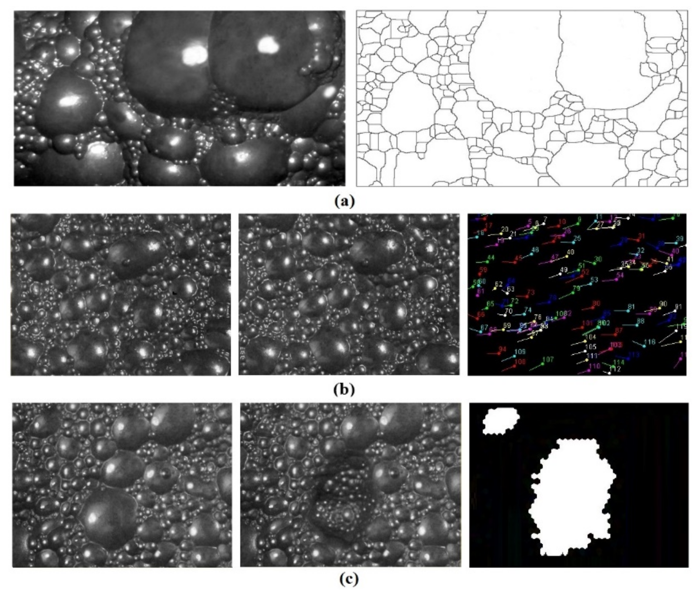
The average of the gray, RGB, HSB (hue, saturation and brightness) and lab values were extracted from images to describe the froth color descriptors. Furthermore, based on each gray level co-occurrence matrix (GLCM), four texture features (entropy, contrast, inverse different moment (IDM), and angular second moment (ASM) or energy) were selected to describe the froth surface textural characteristics. A watershed technique was applied to measure the bubble size distribution, roundness (circularity) and aspect ratio (AR) (Figure 3a). The bubble burst rate (stability) and froth velocity (transport rate) which are dynamic descriptors were extracted from an image pair. The pixel tracing algorithm was applied to quantify the froth speed (pixel/s) between the consecutive frames (Figure 3b). The bubble burst rate was computed by finding the difference between two consecutive frames (Figure 3c). The particular implementation of the image processing techniques to extract the froth features offline was presented by Nakhaei et al. [38].

Since the purpose of this study was to find a valid model to describe the relationship between sulfur recovery and froth surface characteristics, the flotation experiments were performed on a wide range of operational variables. Therefore, the most important operational variables including aeration rate, solid percentage, froth height, chemicals dosage and pulp pH were changed for each run. A total of 99 experiments were designed and performed. The technical parameters of the reverse in-column flotation experiments are given in

Table 1. Variables and levels used in column flotation experiments.

Variable	Range
Collector concentration (g/t)	40–220
Frother concentration (g/t)	60–230
Froth height (cm)	10–40
Air flowrate (cm/s)	1.3–1.9
Solids (%)	10–35
Pulp pH	2.5–8

. The values of sulfur recovery spread out over a large range, as shown by the high values of the standard deviations, due to the different conditions applied in the flotation process (

Table 2. The statistical measures of sulfur recovery (the output variable).

Metallurgical Factor	Maximum	Minimum	Average	SD
Recovery (%)	85.08	6.53	49.28	18.56

).

Table 3. Descriptive statistics of the froth features obtained at different operating conditions as inputs for the k-means algorithm, regression and BPNN models.

Features	Maximum	Minimum	Average	Features	Maximum	Minimum	Average
Gray level	112	74	86.36	Energy (0º)	1 × 10−3	2.5 × 10−4	5.2 × 10−4
R	136	79	95.3	Contrast (0º)	260	45.81	128.5
G	111	78	89.03	IDM (0º)	0.39	0.15	0.23
B	101	63	76.01	Entropy (0º)	10.05	7.75	8.50
Hue	0.36	0.11	0.25	Bubble size	50.97	5.6	30.80
Saturation	0.41	0.19	0.28	Aspect ratio	1.75	1.10	1.43
Brightness	0.53	0.33	0.39	Circularity	0.81	0.34	0.51
L	45.4	33.66	37.68	Speed	26.01	10.77	16.41
a	10.44	−6.3	−0.17	Stability	85.02	57.88	74.31
b	15.71	4.62	9.2

summarizes the values of the input dataset (froth characteristics) for the k-means algorithm, regression, and BPNN models. This dataset was extracted offline by applying a wide range of operational conditions to form a robust predictive model for sulfur recovery estimation.

According to the expert experiences, the process conditions (sulfur removal) can be sorted into six groups: A–F (

Table 4. Different froth classes in CNN model under various operating conditions.

Type	Sulfur Recovery (%)	Class Label	Number of Images
Very low	≤20	A	180
Low	20–30	B	300
Low–medium	30–40	C	390
Medium	40–50	D	480
Medium–high	50–65	E	1140
High	≥65	F	480

). Each group stands for a specific process condition. A large number of froth images under various operating conditions were collected and directly fed into the CNN model. The training and testing of the CNN model were performed using 2079 and 891 froth images, respectively.

2.3. Models

In a flotation plant, the sulfur content of the concentrate needs to be sampled in the laboratory for analysis and this takes several hours. Consequently, when unexpected events happen, the sulfur content in the iron concentrate may increase with a decrease in the process efficiency. The late detection may lead this phenomenon to last for a long time resulting in economic losses. A soft sensor based on mixed image analysis and mathematical methods can predict the amount of sulfur removal in real-time and thus enable workers to quickly tackle these problems. In this study, the applicability of k-means, MLR, BPNN, and CNN methods for predicting the sulfur removal was compared. The general purpose of using different methods is to find which model most accurately discovers the relationship between inputs and output.

2.3.1. K-Means Clustering

Clustering is an unsupervised learning technique in the area of machine learning, which categorizes objects with high similarity into the same cluster according to a certain distance metric [45,58]. Thus, a cluster is a collection of similar data which are not similar to the data located in other clusters [59,60]. The more similar the objects in the cluster, the better the clustering effect [45]. Among various types of clustering methods, k-means is one of the most widely used clustering algorithms. In this work, the k-means algorithm was employed because of its high efficiency and simplicity in pattern recognition of massive data. The k-means algorithm splits a dataset into K discrete non-overlapping clusters. The clustering is performed by minimizing the sum of squares of distances between the center and the data in each cluster [61]. Details of the k-means algorithm procedure are presented in [47,61].

The simplest procedure of the k-means algorithm can be described as follows [48,62]: (1) Choose random initial clusters centroids. (2) Compute the Euclidean distance between each object to each cluster centroid according to Equation (1):

$$D=\sqrt{{{\displaystyle \sum }}_{i=1}^n{{\displaystyle \sum }}_{j=1}^m{\left|X_{ij}-C_j\right|}^2}$$

(1)

where D is the Euclidean distance; n is the number of data; m is the number of dimensions; X_ij is stated as the j dimensionality of the i-th data; Cj is the j dimensionality of the cluster center [48].

(3) Assign data points to one of the clusters on the basis of the proximity to the centers. (4) Assign new centroids for each cluster by averaging the data of each cluster. (5) Return to step 2 and repeat the process until convergence is obtained.

In the current study, the k-means algorithm was applied to cluster the froth features’ dataset into specific groups (based on a given k value) depending on the flotation recovery (low to high). The algorithm described above was implemented based on the code in Python software (3.1, Python Software Foundation manufacturer).

The efficiency of each cluster is evaluated using the accuracy criterion. The accuracy of each cluster is the percentage of observations of the dataset that is correctly classified by the model used. This can be written as:

$$Accuracy=\frac{CN}{CN+FN}\times 100$$

(2)

where CN is the number of correct responses, FN is the number of false responses.

2.3.2. Multiple Linear Regression

MLR is one of the mathematical methods used to describe the linear relationship between the independent variables and dependent variables [63]. MLR is used when the value of a specific variable can be estimated based on the values of other variables. In MLR, the model is fit by minimizing the sum of squares of the difference between the observed and fitted values. The linear equation is as follows [64]:

$$Y=C_0+C_1{x}_1+C_2{x}_2+\cdots +C_n{x}_n+\epsilon$$

(3)

where Y corresponds to the output variable, X_i is the independent variables, C_i is the regression coefficients, and ε represents the error term.

The froth features were taken as input variables for the MLR model to predict the sulfur recovery. In the MLR modeling, 85% of data was randomly used for computing the equation (84 runs) and 15% for testing (15 runs). The MLR analysis was performed using the SPSS 27 software (Property of IBM Corp.).

2.3.3. Backpropagation Neural Network

NNs are nonlinear computational methods that have been successfully used in various fields of science and technology over the past decade [65,66,67]. The main feature of the NN is its ability to learn the complex relationships between input and output data. The main advantages of the NN models are as follows: (1) It only considers the input and output data without referring to the process phenomenology; and (2) it has a generalization ability to accurately estimate the outputs corresponding to a new dataset that were not applied for training of the model [39,68].

NN is a complex network structure consisting of three or more layers to learn the nonlinear relationship between input and output data. The layers are processed with a large number of interconnected neurons. Each neuron, has an associated weight and bias. Figure 4 shows the NN structure, where X₁ and X_n are the inputs. W is the corresponding connection weight, b is the bias and Y is the output.

The modelling process is as follows: The first stage consists of choosing the network configuration and the number of nodes in the layers, and giving the random value of the weight and the bias matrixes. In the second stage, the input and the output matrixes are entered. In the third stage, the hidden layer output matrix and the output matrix of the last layer are calculated; The next step is to compute the difference between the output of the model and the actual output; if the error value is within the specified range, the training ends; otherwise, the fifth stage is continued. In the fifth stage, the error is back-propagated and the data are forwarded and the weight and bias matrixes are updated.

The dataset of the flotation tailing froth features is applied to train the network for predicting the amount of sulfur removal from iron ore concentrate in the column flotation process. In this study, 74 of 99 (75%) items in the dataset were used in training and the rest 25 (25%) in the test and validation of the network. The training process was carried out by applying the backpropagation algorithm with the Levenberg–Marquardt training method. The neural net fitting toolbox from MATLAB program, version R2022, was used to make the code for the NN. The tansig, and purelin activation functions were used in the hidden layer and the output layer, respectively. These complex functions offer the NN model the ability to learn both linear and nonlinear relationships between the inputs and the outputs.

The proper choice of the number of neurons in the hidden layer is an important task. According to the literature, as long as the number of neurons in the hidden layer is appropriately specified within reasonable limits, a three-layer BPNN can be effectively applied to model a wide range of complex problems [69]. Too many neurons may result in increasing the computational time or overlearning so that the NN loses its ability to generalize the patterns present in the training dataset. On the other hand, very few numbers of neurons may cause underfitting so that the model is not complex enough to capture patterns in the data [70,71].

In general, it is not possible to comment definitively on the number of neurons required for a proper network execution. The best number of hidden neurons was determined by trial and error, based on the evaluation of the mean square error (MSE). An empirical formula has been proposed [72] to find the number of hidden neurons:

$$n_h=\sqrt{\left(n_i+n_o\right)}+c$$

(4)

where $n_h$, $n_i$ and $n_o$ are the number of neurons in hidden, input and output layers, respectively. c is an adjustment constant ranging from 1 to 10. In this article, based on Equation (4), the number of hidden neurons was examined from 6 to 16 to determine the optimal value.

Performance Evaluation of the NN and the MLR Models

Three statistical indexes, including correlation coefficient (R²), root mean square error (RMSE) and error percentage (E), were applied to assess the performance of the developed NN and MLR models in order to find whether there was any significant difference in their performance. These three performance indicators are calculated as follows [73,74]:

$$R^2={\left[\frac{n({\displaystyle \sum }XY)-({\displaystyle \sum }X)({\displaystyle \sum }Y)}{\sqrt{(}n{\displaystyle \sum }{X}^2-({\displaystyle \sum }X{)}^2)(n{\displaystyle \sum }{Y}^2-({\displaystyle \sum }Y{)}^2)}\right]}^2$$

(5)

$$RMS={\left[\frac{1}{n}{\displaystyle \sum }{(X-Y)}^2\right]}^{\frac{1}{2}}$$

(6)

$$E=\frac{1}{n} \sum \left|\frac{Y-X}{X}\right|$$

(7)

In these equations, X represents the measured values, Y is the estimated values, and n is the number of data. The correlation coefficient can determine how the network output changes according to the actual values, and when it is equal to one, there is a complete correlation between the estimated and the measured values. The lower RMSE and error percentage values represent the more accurate estimation results.

2.3.4. Convolutional Neural Network

CNN is considered to be one of the most popular NNs for image classification problems. Basically, a CNN is a kind of feedforward NN which comprises two main sections: The first section (feature extraction) comprises input layer, convolution and pooling layers and the second section (classification) consists of a dense (flattened) layer, fully connected layers and an output layer [75]. Figure 5 illustrates the architecture of a typical CNN.

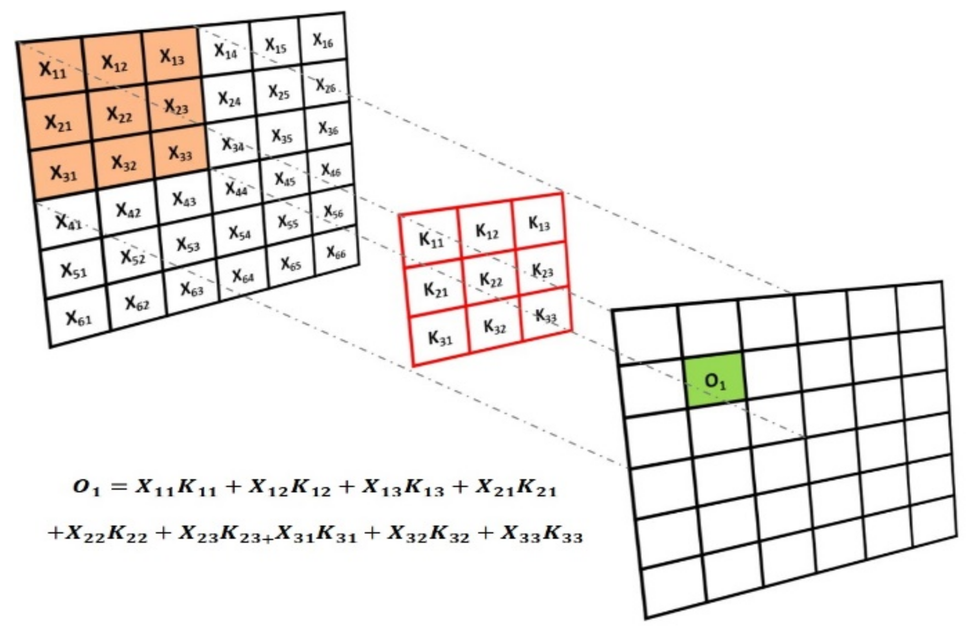
The convolutional layer (CL) is the main part of a CNN which extracts features by convoluting the kernel (filter) over an original image (matrix). The filter works by moving a window from left to right and top to bottom to multiply and sum each position of the source pixel (Figure 6). Each convolution layer adopts a 3 × 3 filter with a stride of 1. ReLU (rectified linear unit) is used as an activation function after each CL. ReLU is always levelled as 0 and 1. The pooling layer decreases the dimension of feature maps while keeping the most important information to avoid overfitting [76]. It is generally situated between consecutive CLs. The maximum pooling function adopts a matrix of size 2 × 2 (Figure 7).

After the pooling layer, the output feature maps are flattened in the dense layer by transforming the input from multidimensional space to a one-dimensional array of numbers to smooth the connection of nodes in the fully connected layer. The classification of the input image is performed in the classification layer with the ability to adjust weights. The number of nodes in the classification layer corresponds to the number of classes in the output.

Many popular CNN architectures have been developed such as LeNet, GoogleNet, VGG16, ResNet, and AlexNet to solve machine vision-based problems [65]. In this study, ResNet18 was selected. MATLAB 2021a (The MathWorks, Inc. protected by U.S and international patents), with Machine toolbox deep neural network designer, was used in this experiment.

3. Results and Discussion

3.1. Correlation between Froth Features and the Process Metallurgical Performance

The predictive model performance depends on the data nature, and the variable selection [77]. Feature selection should be considered to find the best set of variables to build useful predictive models.

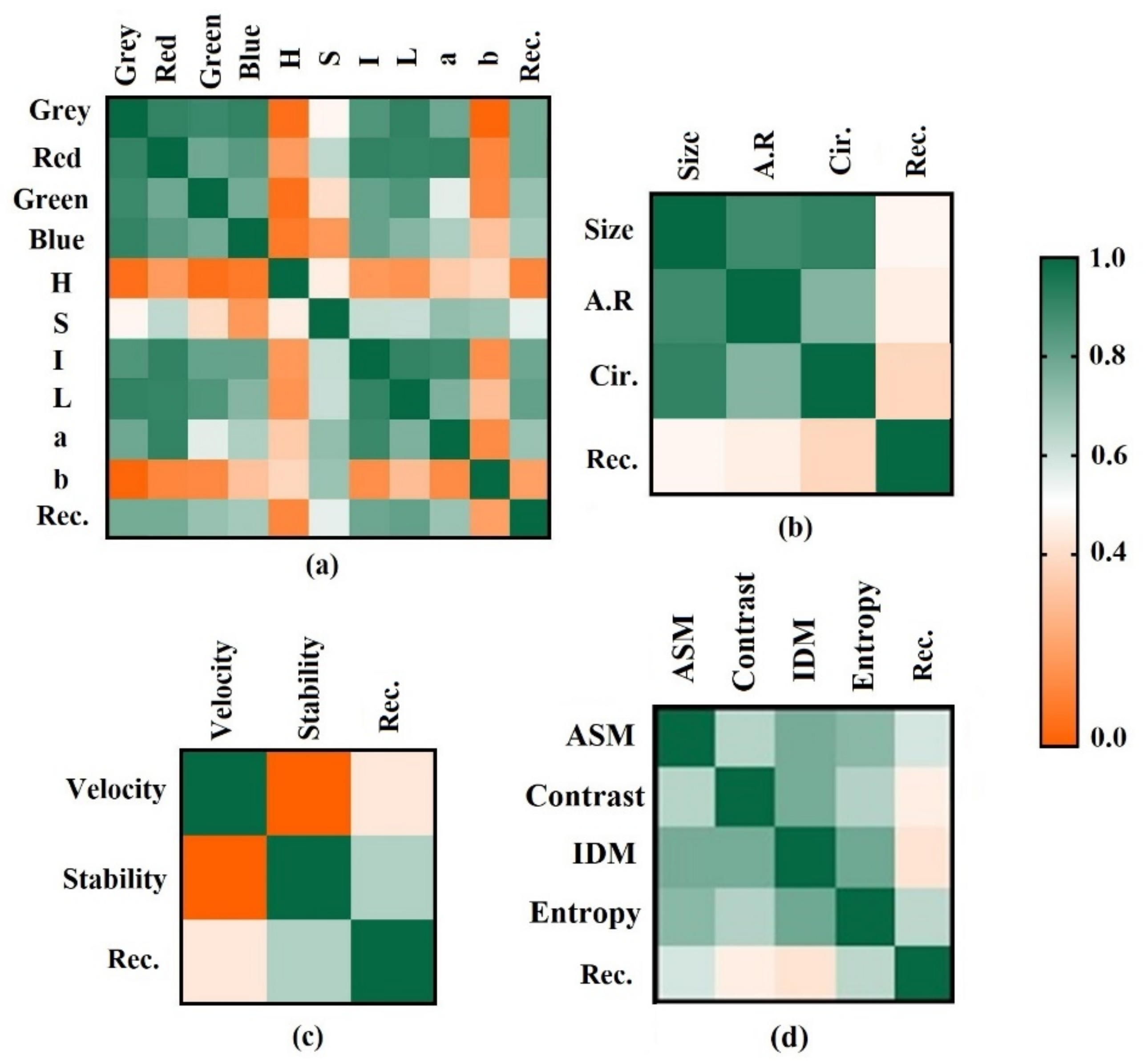
The correlation coefficient is a statistical measure that is commonly used to calculate the strength of the relationship between two variables [78]. In order to select the appropriate variables and minimize the required dataset, the Pearson correlation coefficients between the froth features and the sulfur recovery were implemented. The values of the correlation matrix between the froth images features and the recovery are shown in Figure 8. As shown in the heatmap, color features obtained from the froth images except H and b were strongly associated with the amount of sulfur removal, showing almost similar correlation coefficients. As a result, these parameters were suitable for the sulfur recovery estimation. Furthermore, there were very weak correlations between the H, b and the recovery. Therefore, these two features were excluded from the model predictors due to having a low contribution rate.

The color characteristics of the froth images are more related to the process performance than to the geometric properties of the bubbles. Figure 8d shows the correlation values between the textural properties of the froth images and the process performance factor. There was a significant correlation between the textural features and the recovery. Among the textural properties, the entropy and energy had a higher correlation with the sulfur removal values. According to the heatmap, both geometric features and dynamic factors were most associated with the recovery. The froth stability relative to the velocity had a higher correlation with the process output variable.

Although the results of the correlation matrix between the amount of sulfur removal and the froth visual properties showed that these features are somewhat in line with expectations, the interaction between the factors may obscure the results. Therefore, the use of nonlinear models for process modelling is justifiable. The input and output variables of the proposed models for prediction of the output parameter are shown in Figure 9.

3.2. Sulfur Removal Estimation Based on K-Means Algorithm

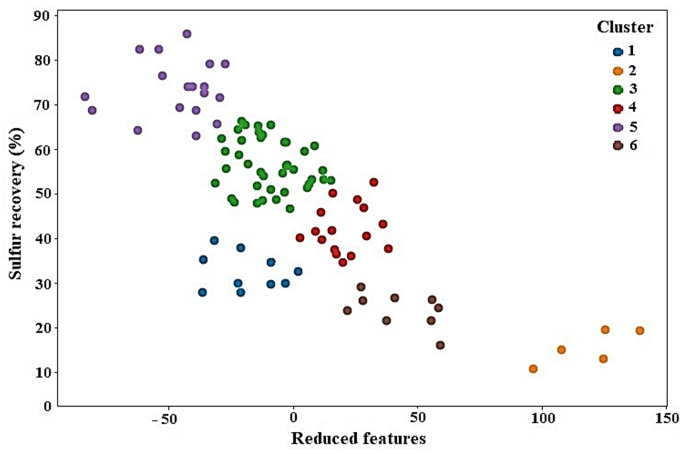
In this study, the k-means algorithm was applied to cluster the froth image features using Python software. The effect of the number of clusters (five and six) was examined. According to the results of this study, a model with six clusters was optimal. The clusters of samples based on k-means algorithm are visualized in Figure 10. The samples were classified into the different clusters with different colors. It is clear that the k-means algorithm was able to classify the dataset. The number of samples in each cluster is given in

Table 5. The number of samples in each cluster.

Cluster	Number of Samples in Cluster
1	10
2	5
3	41
4	16
5	18
6	9

. It can be seen that clusters 3 and 2 had the highest and lowest populations, respectively.

The statistical results obtained by applying the k-means method are shown in

Table 6. Statistical results of predicted values in each cluster.

Cluster	Max.	Min.	Average	SD	Type	Sulfur Recovery (%)
1	37.97	27.91	32.00	3.39	Low–medium	30–40
2	20.57	10.92	15.88	4.14	Very low	≤20
3	66.42	44.06	56.40	6.06	Medium–high	50–65
4	52.62	35.05	42.05	5.42	Medium	40–50
5	87.28	63.73	73.74	6.56	High	≥65
6	29.22	17.08	24.34	3.65	Low	20–30

. According to the results of the flotation experiments, the sulfur recovery was split into six clusters, which were too low, low, low–medium, medium, medium–high and high, as shown in Table 6. For example, cluster 5 was characterized by the highest level of sulfur recovery (average = 73.74%). Clusters 3 and 2 were characterized by the medium–high and the very low level of recovery, respectively. In other words, the average of sulfur recovery in cluster 3 was higher than the average of the corresponding recovery in cluster 2.

The accuracy measure clarifies how well the k-means algorithm was able to group the samples with similar features in the same cluster. To evaluate the errors, it was necessary to check the members of each cluster to see if they were properly classified. The efficiency of each cluster was evaluated using the accuracy criterion (Equation (1)). As shown in

Table 7. The accuracy of each cluster.

Metallurgical Factor	Cluster
	1	2	3	4	5	6
Misclassification	2	0	7	6	2	1
Classification accuracy (%)	80	100	83	63	89	89

, the results of the k-means algorithm almost matched the results of the actual classification. Results demonstrated that the relationships between the froth characteristics and recovery were successfully modelled using the k-means method with rational errors. In general, the clustering results confirmed the principle that sulfur recovery is greatly affected by froth features. The froth features classification could estimate the sulfur recovery more accurately than human workers, avoiding the large fluctuation caused by the personal decisions of different workers. The proposed classifier could be used to cluster other data whose class label is not specified.

3.3. Sulfur Removal Estimation Based on MLR

To predict the amount of sulfur removal from iron ore concentrate, the MLR model was obtained by processing the full data, as shown in Figure 9. The data were split 85:15 into training (to constitute the regression equation) and test data sets. The results of ANOVA for the regression model are shown in

Table 8. Results of ANOVA for regression model.

Sums of Squares Regress	df Regress	Sums of Squares Residual	df Residual	Mean Squares Regress	Mean Squares Residual	F	P-Level
25,256.54	17	3772.41	66	1485.69	57.16	25.99	0.00

. The model is shown in the following equation:

$$\begin{array}{c}SE=212.04+0.204\left(Grey\right)-1.25\left(Red\right)-1.23\left(Green\right)+0.30\left(Blue\right)-106.71\left(S\right)\\ +361.62\left(I\right)+0.66\left(L\right)-1.35\left(a\right)+\mathrm{62,409.34}\left(ASM\right)-0.133\left(Contrast\right)\\ -164.25\left(IDM\right)-5.99\left(Entropy\right)-0.58\left(Buble size\right)-13.34\left(AR\right)\end{array}$$

(8)

The relationship between measured and calculated values using the proposed mathematical model in Equation (8) is presented in Figure 11. The multivariable regression equation predicted the sulfur recovery with a correlation coefficient of 0.92. The comparison of the actual values and the estimated values for sulfur recovery in the validation stage is presented graphically in Figure 12.

According to Figure 11, the R values in the training and validation data set for sulfur recovery were 0.91. The descriptive statistics of the differences between the measured and estimated values for the evaluation data are given in

Table 9. Descriptive statistics of errors between actual and BNN predicted values for the test data.

Variables	Minimum	Maximum	Mean	RMSE	Error Percentage
Prediction error	−11.02	12.14	1.04	6.82	15.4

. Although the MLR has been stated as a capable tool for data modelling, it could not accurately describe the sulfur recovery within the entire process variables space (RMSE = 6.82). This may be due to the complexity of the selected data covering a wide range of operational conditions. Thus, the ANN model was examined as an alternative method and is discussed in the next section.

3.4. Sulfur Removal Estimation Based on BPNN Model

The desulfurization of iron ore concentrate by the column flotation process is highly nonlinear and complicated [34]. The main objective of the current study was to combine image analysis methods with an intelligent predictive model such as NN to forecast the amount of sulfur removal from the iron ore concentrate.

As stated, the visual properties of the flotation froth were included in the input layer and the sulfur recovery in the output layer. The total 99 experimental data were randomly divided into three subsets as training, testing and validation. The training data (74 runs) were used by BPNN to learn how to map the inputs to the output by updating the network weights. The validation data (10 runs) were applied to assess the quality of the model. The ultimate check on the performance and generalization ability of the trained model was performed using testing data (15 runs).

BPNNs with at least one hidden layer are able to effectively estimate any function with the appropriate approximation, as long as the number of hidden neurons is appropriately determined. In the hidden layer, only the number of neurons determines the structure of the network and plays a major role in a network capability. Thus, if the number of neurons is small, the model does not accurately reflect the nonlinear mapping between inputs and outputs. On the other hand, if the number of middle layer neurons is too large, the model becomes overtrained and loses its generalizability [79,80]. To choose the best structure, the number of neurons in the hidden layer was changed to achieve minimum MSE.

The training settings of the BPNN model in this study are summarized as follows: number of input nodes: 17, number of hidden neurons: from 6 to 16, number of output nodes: 1, number of epochs: 1000. As stated in the literature [81], unlike changing the number of hidden nodes, changing the activation function does not have a significant effect on the model performance and results with similar MSE and R. The tangent sigmoid and linear activation functions were used in the hidden and output layers, respectively.

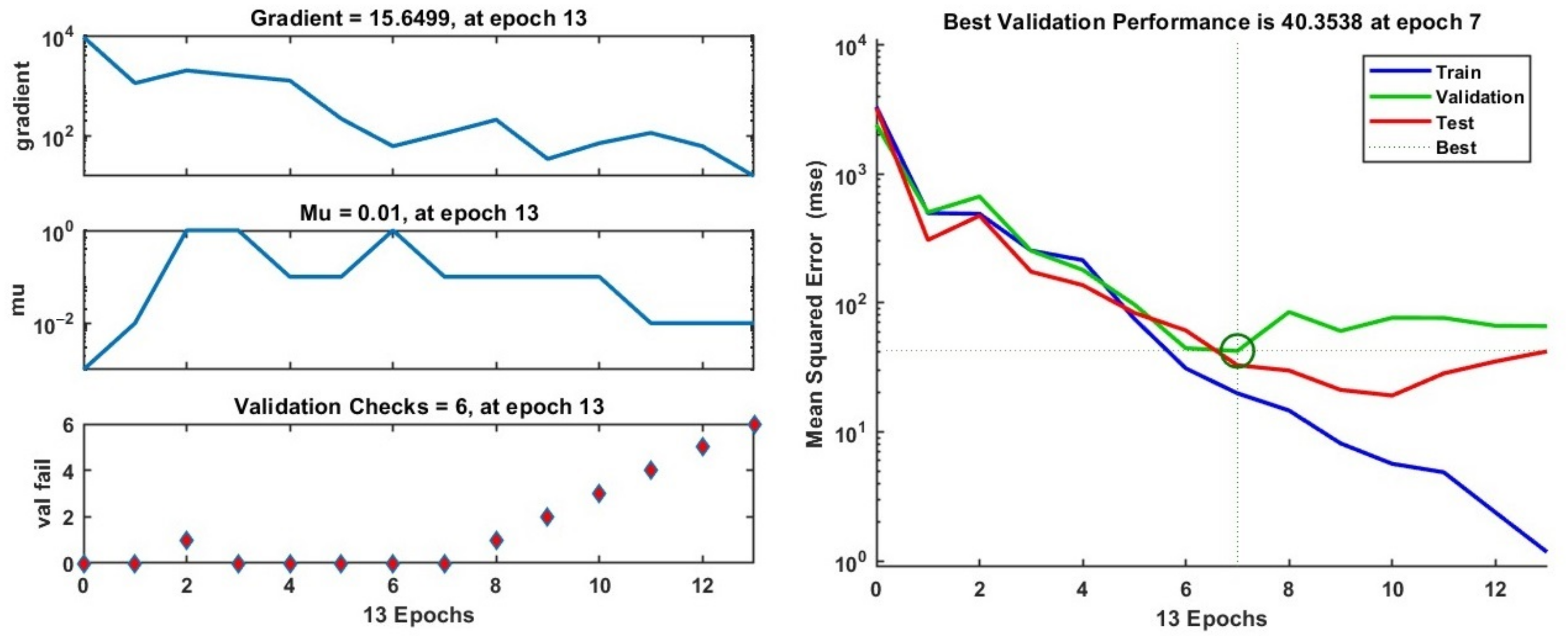
The BPNN model consisting of 10 neurons in the hidden layer gave the lowest MSE error among all the models studied. The network’s performance in the training stage is shown in Figure 13. In the training stage, Mu first increased and then dropped, then fell to 0.01, and remained stationary, which shows that the model had reached its optimum state. The number of validation checks, which describes the number of consecutive iterations that the validation performance fails to reduce, was equal to six. In other words, if the number of validation checks reaches six, the training phase will stop.

Figure 13 shows the MSE variation of the training, validation and testing stages versus the iteration number. As shown in this figure, the large values for the MSE gradually reduced to a smaller value as the weights were updated. Training stage stopped at the seventh epoch, i.e., after epoch seven, there was no significant improvement in the performance of the model. The best validation performance was 48.98 at epoch seven, and after six error iterations (validation checks), the process stopped at epoch thirteen. In epoch seven, the MSE values for training and testing phases were 18.87 and 31.83, respectively, implying a good stable network behavior.

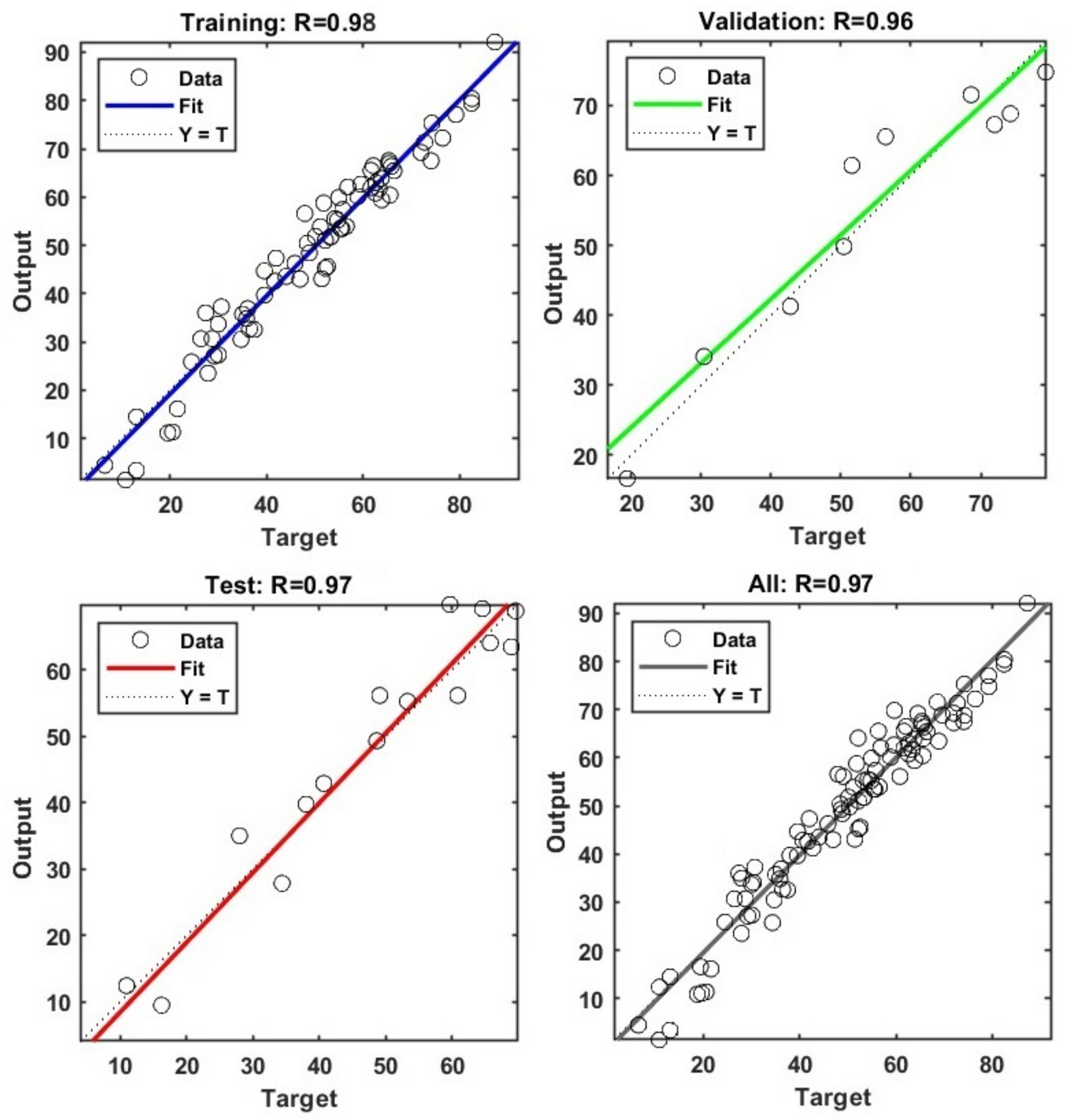
The comparison between the actual and predicted values of the sulfur recovery during training, validation, and testing stages is displayed in Figure 14. The dashed line shows the perfect result, i.e., outputs are equal to targets, while the solid line represents the best fit linear regression.

In the training stage, the predicted data obtained from the BPNN modeling were close to the actual data with a correlation of R = 0.98. Figure 14 shows the good fit attained in both the validation and testing of the proposed model (R values above 0.96). Despite the high variability and wide range of the output data, the overall R of the model was 0.97, which showed the appropriateness of the training, testing, and validity. From these comparison plots, it can be concluded that the BPNN is appropriately trained and shows consistency in forecasting sulfur recovery. The R values obtained from this BPNN model are higher than those reported in other studies in the literature for the prediction of metallurgical performance of the flotation process [19,36,82]. The novelty and superiority of the proposed BPNN model are its highest accuracy compared to the previously reported models to predict the metallurgical performance parameters of the flotation process.

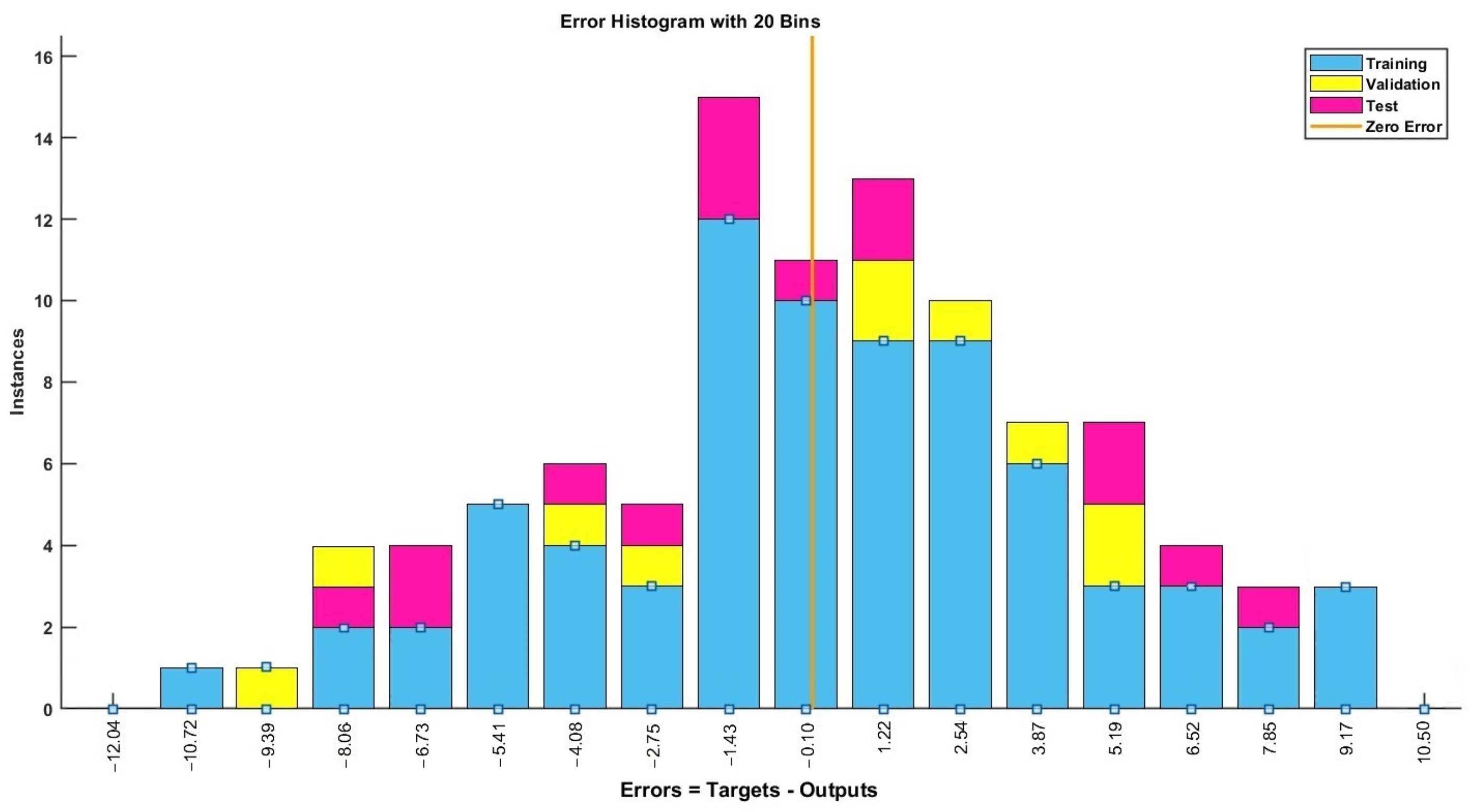
The BPNN error histogram (differences between actual and predicted values) for the prediction of sulfur removal is illustrated in Figure 15. It can be observed that most of the errors were distributed between −1.43 and 2.54. Furthermore, the validation set and test set had similar behavior with no occurrence of overfitting. The comparison of the predicted recoveries with the measured values in the testing phase is shown in Figure 16. The values estimated by utilizing the BPNN model were very close to the actual measurements. The descriptive statistics of the errors in the testing stage (

Table 10. Descriptive statistics of errors between actual and BPNN predicted values for the test data.

Variables	Minimum	Maximum	Mean	RMSE	Error Percentage
Prediction error	8.06	−7.59	0.57	4.84	11.29

) confirmed that the BPNN model based on selected froth features was able to estimate the sulfur recovery quite precisely and satisfactorily. In the testing phase, the R, RMSE, and percent error values were obtained as 0.97, 4.84 and 11.29%, respectively, which confirmed a precise and robust prediction of the experimental data.

It was demonstrated that a well-trained BPNN model based on froth features could be used to predict sulfur recovery from iron ore concentrate by column flotation without needing more experimental study requiring much time and high experiment costs.

3.5. Sulfur Removal Estimation Based on CNN

To classify the six groups of froth data, the ResNet18 deep learning classification method was used. The CNN has 71 layers containing input, convolutional, pooling, fully connected, ReLU, batch normalization, softmax and output layers. The layer structure of the proposed CNN is given in Figure 17.

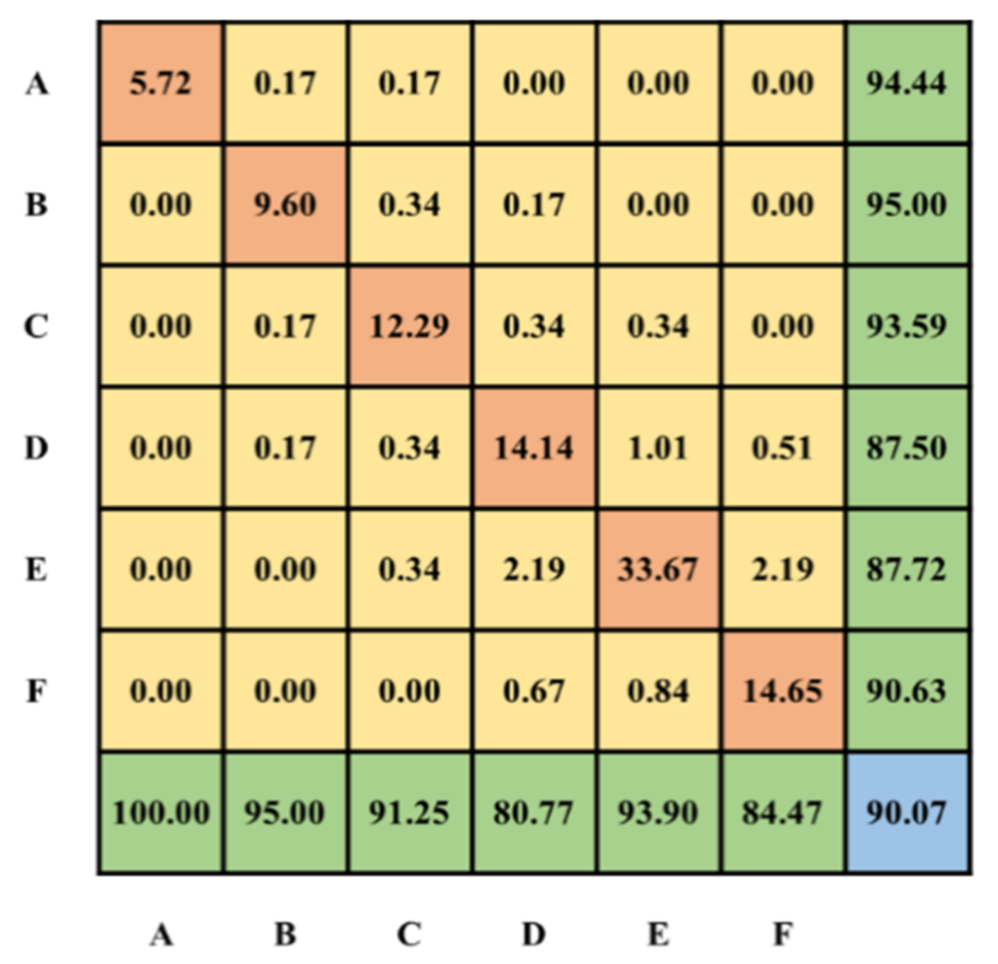
Figure 18 illustrates the confusion matrices of the CNN model in the classification process. A confusion matrix explains the estimation results of a classifier. The diagonal elements represent the number of correct predictions, while the off-diagonal elements represent incorrect estimations. This figure shows that the classification accuracy of the CNN for six froth classes was high, indicating that the model could provide an accurate prediction of the flotation performance (the amount of sulfur removal). The bottom and right values display the overall accuracy of the classification model. The prediction accuracy using this deep learning model was 90% which was much higher than the k-means algorithm.

The results showed that the CNN model was suitable for finding the process conditions of the column flotation in desulfurization of iron ore concentrate with high accuracy and efficiency. For example, if the froth images are categorized in Class A, Class B, or Class C, it is a sign that the current condition is abnormal. In this circumstance, the plant workers need to regulate the operating factors to achieve the desired performance.

3.6. Comparison of MLR, K-Means, BPNN and CNN Models

The results showed that all the proposed models, k-means, MLR, BPNN, and CNN, could be considered for sulfur removal prediction in the desulfurization of iron ore concentrate using flotation froth images. However, when different statistical results such as R, RSME, and percent error were examined, it was clear that the BPNN and CNN predicted values were more accurate than those of the MLR and k-means models.

The total accuracy of the CNN and k-means algorithms were 91% and 82%, respectively. In the k-means algorithm, regression and BPNN models, the froth features were firstly extracted offline through image analysis techniques and then they were entered into the models, whereas in the CNN model the froth images were directly fed into the model. Since, the traditional predictive models were built based on off-line feature extraction techniques, the training time for evaluation of the models was ignored. So, it can be concluded that the CNN and BPNN were able to categorize the froth images with high performance.

The BPNN and CNN models were found to be more successful where nonlinear and complex relationships were involved in the system, such as the desulfurization process of iron ore concentrate using the column flotation process. Thus, it was possible to establish a complex relationship between sulfur recovery and froth flotation features using the BPNN and CNN models with an excellent accuracy level.

It is important to note that sometimes BPNN does not represent the most cost-effective solution. In some cases, the interpretability of the network and weights may be difficult, the determination of the optimum structure and parameters may be troublesome, and the convergence of the training algorithm may be endless [81]. In these situations, MLR models can have advantages in terms of accuracy, variability, and model creation; therefore, its choice is preferred [83].

4. Conclusions

In the iron reverse flotation process, the amount of sulfur removal and the quality of flotation concentrate are usually judged according to the froth’s surface appearance. Visual assessments by workers are challenging tasks and often inaccurate; in practice, they can only be performed at a given time. A machine vision system for monitoring and control of the operating conditions of the flotation process can be a great help for workers and iron and steel producers. Therefore, to forecast the amount of sulfur removal from the iron concentrate in the flotation process, soft-sensor models based on extracted froth features were proposed.

A total of 99 flotation column experiments were conducted in a wide range of different operating conditions and the froth features were extracted for each run. In this study, the abilities of four algorithms, including multiple linear regression (MLR), the k-means algorithm, the backpropagation neural network (BPNN), and the convolutional neural network (CNN) to predict the sulfur recovery, were examined and compared. In the first three models, the different froth features such as color, bubble shape and size, texture, froth stability, and velocity were primarily extracted offline through image processing techniques and then they were fed into the models, whereas in the CNN model the froth images were directly fed into the model.

The results showed that among the four algorithms implemented, the three-layer BPNN and the CNN models outperformed the MLR and k-means techniques when predicting sulfur recovery. The best NN model was a backpropagation network (topology 17-10-1) using a Levenberg–Marquardt algorithm for the training step, showing R = 0.97, RMSE = 4.84 and percent error = 11.29%. The total accuracy of the CNN and k-means algorithms were 91% and 80%, respectively. Therefore, the sulfur recovery, which is the most important parameter for control purposes of the flotation process, can be accurately predicted from the froth surface appearance by the BPNN and CNN models.

Considering the accuracy and time consumed in measuring the metallurgical parameters of the flotation process, with the use of BPNN and CNN models, satisfactory results can be predicted rather than measured in the laboratory which thereby reduces the testing time and cost. As a result, it can be confirmed that such modelling studies pave the way to find an alternative to the on-stream analyzer, such as XRF, which is costly and not widely available.

In the future, the performance of the proposed models can be improved if more machine learning techniques are tested on larger datasets. Finally, future studies should concentrate on the validation and generalization of the proposed models in an industrial flotation process.

References

1. Corin, K.C.; McFadzean, B.J.; Shackleton, N.J.; O’Connor, C.T. Challenges related to the processing of fines in the recovery of platinum group minerals (PGMs). Minerals 2021, 11, 533. [Google Scholar] [CrossRef]
2. Nakhaei, F.; Irannajad, M. Sulphur removal of iron ore tailings by flotation. J. Dispers. Sci. Technol. 2017, 38, 1755–1763. [Google Scholar] [CrossRef]
3. Nakhaei, F.; Irannajad, M.; Mohammadnejad, S. Comparison of conventional and column flotation performance for desulfurization of iron ore concentrate. New Find. Appl. Geol. 2019, 13, 55–66. [Google Scholar]
4. Jovanovíc, I.; Miljanovíc, I. Contemporary advanced control techniques for flotation plants with mechanical flotation cells—A review. Miner. Eng. 2015, 70, 228–249. [Google Scholar] [CrossRef]
5. Pu, Y.; Szmigiel, A.; Apel, D.B. Purities prediction in a manufacturing froth flotation plant: The deep learning techniques. Neural Comput. Applic. 2020, 32, 13639–13649. [Google Scholar] [CrossRef]
6. Jing, Z.; Jinling, N.; Yong, Z. Prediction of concentrate grade and recovery rate of tailings in the process of production based on chaotic ant colony algorithm. In Proceedings of the 2018 Chinese Control and Decision Conference (CCDC), Shenyang, China, 9–11 June 2018; pp. 5308–5313. [Google Scholar] [CrossRef]
7. Tang, M.; Zhou, C.; Zhang, N.; Liu, C.; Pan, J.; Cao, S. Prediction of the ash content of flotation concentrate based on froth image processing and bp neural network modeling. Int. J. Coal Prep. Util. 2021, 41, 191–202. [Google Scholar] [CrossRef]
8. Nakhaei, F.; Sam, A.; Mosavi, M.R.; Nakhaei, A. Prediction of XRF analyzers error for elements on-line assaying using Kalman Filter. Int. J. Min. Sci. Technol. 2012, 22, 595–601. [Google Scholar] [CrossRef]
9. Nakhaei, F.; Abdollahzade, A.; Irannejad, M. Presenting a method for examining the measurement system construction of mineral processing complicated circuits: Extracting observable variables and conducting mass balance. J. Anal. Numer. Methods Min. Eng. 2013, 3, 77–88. [Google Scholar]
10. Brooks, K.S.; Koorts, R. Model predictive control of a zinc flotation bank using online x-ray fluorescence analysers. IFAC-Papers OnLine 2017, 50, 10214–10219. [Google Scholar] [CrossRef]
11. Zhang, J.; Tang, Z.; Xie, Y.; Ai, M.; Gui, W. Convolutional memory network based flotation performance monitoring. Miner. Eng. 2020, 151, 106332. [Google Scholar] [CrossRef]
12. Jahedsaravani, A.; Marhaban, M.H.; Massinaei, M. Application of statistical and intelligent techniques for modeling of metallurgical performance of a batch flotation process. Chem. Eng. Commun. 2016, 203, 151–160. [Google Scholar] [CrossRef]
13. Vieira, S.; Sousa, J.; Durão, F. Fuzzy modelling strategies applied to a column flotation process. Miner. Eng. 2005, 18, 725–729. [Google Scholar] [CrossRef]
14. Bergh, L.G.; Yianatos, J.B. The long way toward multivariate predictive control of flotation processes. J. Process Control 2011, 21, 226–234. [Google Scholar] [CrossRef]
15. Shean, B.J.; Cilliers, J.J. A review of froth flotation control. Int. J. Miner. Processing 2011, 100, 57–71. [Google Scholar] [CrossRef]
16. Nakhaei, F.; Irannajad, M. Application and comparison of RNN, RBFNN and MNLR approaches on prediction of flotation column performance. Int. J. Min. Sci. Technol. 2015, 25, 983–990. [Google Scholar] [CrossRef]
17. Merma, A.G.; Olivera, C.A.C.; Hacha, R.R.; Torem, M.L.; Santos, B.F. optimization of hematite and quartz bioflotation by an artificial neural network (ANN). J. Mater. Res. Technol. 2019, 8, 3076–3087. [Google Scholar] [CrossRef]
18. Geng, Z.; Chai, T.; Yue, H. A method of hybrid intelligent optimal setting control for flotation process. In Proceedings of the Intelligent Control and Automation, 7th World Congress on IEEE, Chongqing, China, 25–27 June 2008; pp. 4713–4718. [Google Scholar]
19. Nakhaei, F.; Mosavi, M.R.; Sam, A.; Vaghei, Y. Recovery and grade accurate prediction of pilot plant flotation column concentrate: Neural network and statistical techniques. Int. J. Miner. Processing 2012, 110–111, 140–154. [Google Scholar]
20. Wang, J.S.; Han, S. Feed forward neural network soft-sensor modeling of flotation process based on particle swarm optimization and gravitational search algorithm. Comput. Intel. Neurosc. 2015, 2015, 1–10. [Google Scholar] [CrossRef] [Green Version]
21. Massinaei, M.; Sedaghati, M.R.; Rezvani, R.; Mohammadzadeh, A.A. Using data mining to assess and model the metallurgical efficiency of a copper concentrator. Chem. Eng. Commun. 2014, 201, 1314–1326. [Google Scholar] [CrossRef]
22. Al-Thyabat, S. Investigating the effect of some operating parameters on phosphate flotation kinetics by neural network. Adv. Powder. Technol. 2009, 20, 355–360. [Google Scholar] [CrossRef]
23. Nakhaei, F.; Irannajad, M.; Mohammadnejad, S. Application of image analysis systems in flotation process. Soft Comput. J. 2021, 5, 66–83. [Google Scholar]
24. Irannajad, M.; Soltanpour, R.; Nakhaei, F. Evaluation of factors affecting carrying capacity of laboratory flotation column treating copper sulfides. Amirkabir J. Civ. Eng. 2019, 51, 725–732. [Google Scholar]
25. Tan, J.; Liang, L.; Peng, Y.; Xie, G. The concentrate ash content analysis of coal flotation based on froth images. Miner. Eng. 2016, 92, 9–20. [Google Scholar] [CrossRef]
26. Li, Z.; Gui, W. The method of reagent control based on time series distribution of bubble size in a gold-antimony flotation process. Asian J. Control 2017, 20, 2223–2236. [Google Scholar] [CrossRef]
27. Nakhaei, F.; Irannajad, M.; Mohammadnejad, S.; Hajizadeh Omran, A. Sulfur content reduction of iron concentrate by reverse flotation. Energy Sources Part A Recover. Util. Environ. Eff. 2019, 1–17. [Google Scholar] [CrossRef]
28. Morar, S.H.; Harris, M.C.; Bradshaw, D.J. The use of machine vision to predict flotation performance. Miner. Eng. 2012, 36–38, 31–36. [Google Scholar] [CrossRef]
29. Nakhaei, F.; Irannajad, M.; Mohammadnejad, S. A comprehensive review of froth surface monitoring as an aid for grade and recovery prediction of flotation process. Part A: Structural features. Energy Sources Part A Recovery Util. Environ. Eff. 2019, 1–23. [Google Scholar] [CrossRef]
30. Bartolacci, G.; Pelletier, P.; Tessier, J.; Duchesne, C.; Bossé, P.A.; Fournier, J. Application of numerical image analysis to process diagnosis and physical parameter measurement in mineral processes—Part I: Flotation control based on froth textural characteristics. Miner. Eng. 2006, 19, 734–747. [Google Scholar] [CrossRef]
31. Ren, C.C.; Yang, J.G.; Liang, C. Estimation of copper concentrate grade based on color features and least-squares support vector regression. Physicochem. Probl. Miner. Processing 2015, 51, 163–172. [Google Scholar]
32. Xu, D.; Chen, X.; Xie, Y.; Yang, C.; Gui, W. Complex networks-based texture extraction and classification method for mineral flotation froth images. Miner. Eng. 2015, 83, 105–116. [Google Scholar] [CrossRef]
33. Núñez, F.; Cipriano, A. Visual information model-based predictor for froth speed control in flotation process. Miner. Eng. 2009, 22, 366–371. [Google Scholar] [CrossRef]
34. Nakhaei, F.; HajizadehOmran, A.; Irannajad, M.; Mohammadnejad, S. Relationship between froth behavior and operating parameters of flotation column. In Proceedings of the XXIX International Mineral Processing Congress (IMPC 2018), Moscow, Russia, 17–21 September 2018. [Google Scholar]
35. Hemmati Chegeni, M.; Abdollahy, M.; Khalesi, M.R. Bubble loading measurement in a continuous flotation column. Miner. Eng. 2016, 85, 49–54. [Google Scholar] [CrossRef]
36. Nakhaei, F.; Irannajad, M.; Mohammadnejad, S. Column flotation performance prediction: PCA, ANN and image analysis-based approaches. Physicochem. Probl. Miner. Processing 2019, 55, 1298–1310. [Google Scholar]
37. Lin, B.; Recke, B.; Knudsen, J.K.H.; Jørgensen, S.B. Bubble size estimation for flotation processes. Miner. Eng. 2008, 21, 539–548. [Google Scholar] [CrossRef]
38. Nakhaei, F.; Iranajad, M.; Mohammadnejad, S. Evaluation of column flotation froth behavior by image analysis: Effects of operational factors in desulfurization of iron ore concentrate. Energy Sources Part A Recovery Util. Environ. Eff. 2018, 40, 2286–2306. [Google Scholar] [CrossRef]
39. Kalyani, V.K.; Pallavika; Chaudhuri, S.; Charan, T.G.; Haldar, D.D.; Kamal, K.P.; Badhe, Y.P.; Tambe, S.S.; Kulkarni, B.D. Study of a laboratory-scale froth flotation process using artificial neural networks. Miner. Process. Extr. Metall. Rev. 2008, 29, 130–142. [Google Scholar]
40. Nakhaei, F.; Irannajad, M.; Yousefikhoshbakht, M. Flotation column performance optimisation based on imperialist competitive algorithm. Int. J. Min. Miner. Eng. 2016, 7, 1–17. [Google Scholar] [CrossRef]
41. Alsafasfeh, A.H.; Alagha, L.; Alzidaneen, A.; Nadendla, V.S.S. Optimization of flotation efficiency of phosphate minerals in mine tailings using polymeric depressants: Experiments and machine learning. Physicochem. Probl. Miner. Processing 2022, 58, 150477. [Google Scholar] [CrossRef]
42. Bu, X.; Zhou, S.; Danstan, J.K.; Bilal, M.; Hassan, F.U.; Chao, N. Prediction of coal flotation performance using a modified deep neural network model including three input parameters from feed. Energy Sources Part A Recover. Util. Environ. Eff. 2022, 1–13. [Google Scholar] [CrossRef]
43. Wang, X.; Song, C.; Yang, C.; Xie, Y. Process working condition recognition based on the fusion of morphological and pixel set features of froth for froth flotation. Min. Eng. 2018, 128, 17–26. [Google Scholar] [CrossRef]
44. Stangierski, J.; Weiss, D.; Kaczmarek, A. Multiple regression models and Artificial Neural Network (ANN) as prediction tools of changes in overall quality during the storage of spreadable processed Gouda cheese. Eur. Food Res. Technol. 2019, 245, 2539–2547. [Google Scholar] [CrossRef] [Green Version]
45. Du, X.; Niu, D.; Chen, Y.; Wang, X.; Bi, Z. City classification for municipal solid waste prediction in mainland China based on K-means clustering. Waste Manag. 2022, 144, 445–453. [Google Scholar] [CrossRef] [PubMed]
46. Zhao, Y.; Peng, T.; Li, K. An improved K-means algorithm based recognition method for working condition of flotation process. Int. J. Syst. Control Inf. Processing 2017, 2, 113–126. [Google Scholar] [CrossRef]
47. Yassin, S.; Pooja, S. Road accident prediction and model interpretation using a hybrid K-means and random forest algorithm approach. SN Appl. Sci. 2020, 2, 1576. [Google Scholar] [CrossRef]
48. Abo-Elnaga, Y.; Nasr, S. K-means cluster interactive algorithm-based evolutionary approach for solving bilevel multi-objective programming problems. Alex. Eng. J. 2022, 61, 811–827. [Google Scholar] [CrossRef]
49. Jansson, N.F.; Allen, R.L.; Skogsmo, G.; Tavakoli, S. Principal component analysis and K-means clustering as tools during exploration for Zn skarn deposits and industrial carbonates, Sala area, Sweden. J. Geochem. Explor. 2022, 233, 106909. [Google Scholar] [CrossRef]
50. Li, Z.; Gui, W.; Zhu, J. Fault detection in flotation processes based on deep learning and support vector machine. J. Cent. South Univ. 2019, 26, 2504–2515. [Google Scholar] [CrossRef]
51. Zhang, W.; Jin, L.; Song, E.; Xu, X. Removal of impulse noise in color images based on convolutional neural network. Appl. Soft Comput. 2019, 82, 105558. [Google Scholar] [CrossRef]
52. Shi, C.; Tan, C.; Wang, T.; Wang, L.A. Waste classification method based on a multilayer hybrid convolution neural network. Appl. Sci. 2021, 11, 8572. [Google Scholar] [CrossRef]
53. Fu, Y.; Aldrich, C. Froth image analysis by use of transfer learning and convolutional neural networks. Miner. Eng. 2018, 115, 68–78. [Google Scholar] [CrossRef]
54. Wen, Z.; Zhou, C.; Pan, J.; Nie, T.; Zhou, C.; Lu, Z. Deep learning-based ash content prediction of coal flotation concentrate using convolutional neural network. Miner. Eng. 2021, 174, 107251. [Google Scholar] [CrossRef]
55. Nakhaei, F.; Irannajad, M.; Mohammadnejad, S. The effect of column flotation operational variables on desulfurization of iron ore concentrate. J. Anal. Numer. Methods Min. Eng. 2020, 9, 43–58. [Google Scholar]
56. Nakhaei, F.; Irannajad, M. Reagents types in flotation of iron oxide minerals: A review. Miner. Processing Extr. Metall. Rev. 2018, 39, 89–124. [Google Scholar] [CrossRef]
57. Liu, X.H.; Liao, Z.H.; Yan, X.H.; Chen, W. Comprehensive recovery of magnetite and pyrrhotite from a low-grade iron ore. Min. Metall. Eng. 2014, 34, 47–51. [Google Scholar]
58. Xu, R.; Wunsch, D. Survey of clustering algorithms. IEEE Trans. Neural Netw. 2005, 16, 645–678. [Google Scholar] [CrossRef] [Green Version]
59. Miri, S.E.; Azadi, M.; Pakdel, S. Development of a duty cycle with K-means clustering technique for hydraulic steering in an instrumented TIBA vehicle. Transp. Eng. 2022, 8, 100114. [Google Scholar] [CrossRef]
60. Rodriguez, A.; Laio, A. Clustering by fast search and find of density peaks. Science 2014, 344, 1492–1496. [Google Scholar] [CrossRef] [Green Version]
61. Minh, H.L.; To, T.S.; Wahab, M.A.; Le, T.C. A new metaheuristic optimization based on K-means clustering algorithm and its application to structural damage identification. Knowl. -Based Syst. 2022, 251, 109189. [Google Scholar] [CrossRef]
62. Yuan, K.; Chi, G.; Zhou, Y.; Yin, H. A novel two-stage hybrid default prediction model with k-means clustering and support vector domain description. Res. Int. Bus. Financ. 2022, 59, 101536. [Google Scholar] [CrossRef]
63. Agha, S.R.; Alnahhal, M.J. Neural network and multiple linear regression to predict school children dimensions for ergonomic school furniture design. Appl. Ergon. 2012, 43, 979–984. [Google Scholar] [CrossRef] [PubMed]
64. Abrougui, K.; Gabsi, K.; Mercatoris, B.; Khemis, C.; Amami, R.; Chehaibi, S. Prediction of organic potato yield using tillage systems and soil properties by artificial neural network (ANN) and multiple linear regressions (MLR). Soil Tillage Res. 2019, 190, 202–208. [Google Scholar] [CrossRef]
65. Zhang, D.; Gao, X. Soft sensor of flotation froth grade classification based on hybrid deep neural network. Int. J. Prod. Res. 2021, 59, 4794–4810. [Google Scholar] [CrossRef]
66. Fu, Y.; Aldrich, C. Flotation Froth Image Recognition with Convolutional Neural Networks. Miner. Eng. 2019, 132, 183–190. [Google Scholar] [CrossRef]
67. Horn, Z.C.; Auret, L.; McCoy, J.T.; Aldrich, C.; Herbst, B.M. Performance of convolutional neural networks for feature extraction in froth flotation sensing. IFAC-Pap. 2017, 50, 13–18. [Google Scholar] [CrossRef]
68. Nandi, S.; Ghosh, S.; Tambe, S.S.; Kulkarni, B.D. Artificial neural–network-assisted stochastic process optimization strategies. AICHE J. 2001, 47, 126–141. [Google Scholar] [CrossRef]
69. Zhang, N.N.; Zhou, C.C.; Pan, J.H.; Xia, W.; Liu, C.; Tang, M.C.; Cao, S.S. The response of diasporic-bauxite flotation to particle size based on flotation kinetic study and neural network simulation. Powder Technol. 2017, 318, 272–281. [Google Scholar] [CrossRef]
70. Çakman, G.; Gheni, S.; Ceylan, S. Prediction of higher heating value of biochars using proximate analysis by artificial neural network. Biomass Conv. Bioref. 2021, 1–9. [Google Scholar] [CrossRef]
71. Lee, K.M.; Zanil, M.F.; Chan, K.K.; Chin, Z.P.; Liu, Y.C.; Lim, S. Synergistic ultrasound-assisted organosolv pretreatment of oil palm empty fruit bunches for enhanced enzymatic saccharification: An optimization study using artificial neural networks. Biomass Bioenergy 2020, 139, 105621. [Google Scholar] [CrossRef]
72. Bu, X.; Xu, Y.; Zhao, M.; Li, D.; Zou, J.; Wang, L.; Bai, J.; Yang, Y. Simultaneous extraction of polysaccharides and polyphenols from blackcurrant fruits: Comparison between response surface methodology and artificial neural networks. Ind. Crops Prod. 2021, 170, 113682. [Google Scholar] [CrossRef]
73. Samani, B.H.; Samani, M.A.; Shirneshan, A.; Fayyazi, E.; Najafi, G.; Rostami, S. Evaluation of an enhanced ultrasonic-assisted biodiesel synthesized using safflower oil in a diesel power generator. Biofuels 2020, 11, 523–532. [Google Scholar] [CrossRef]
74. Wang, W.; Liu, Y.; Bai, F.; Xue, G. Capture power prediction of the frustum of a cone shaped floating body based on BP neural network. J. Mar. Sci. Eng. 2021, 9, 656. [Google Scholar] [CrossRef]
75. Lu, F.; Liang, Y.; Wang, X.; Gao, T.; Chen, Q.; Liu, Y.; Zhou, Y.; Yuan, Y.; Liu, Y. Prediction of amorphous forming ability based on artificial neural network and convolutional neural network. Comput. Mater. Sci. 2022, 210, 111464. [Google Scholar] [CrossRef]
76. Tegegne, A.M. Applications of Convolutional Neural Network for Classification of Land Cover and Groundwater Potentiality Zones. J. Eng. 2022, 2022, 6372089. [Google Scholar] [CrossRef]
77. Asim, Y.; Shahid, A.R.; Malik, A.K.; Raza, B. Significance of machine learning algorithms in professional blogger’s classification. Comput. Electr. Eng. 2018, 65, 461–473. [Google Scholar] [CrossRef]
78. Batabyal, A.K. Correlation and multiple linear regression analysis of groundwater quality data of Bardhaman District, West Bengal, India. Int. J. Res. Chem. Environ. 2014, 4, 42–51. [Google Scholar]
79. Charan, T.G.; Kalyani, V.K.; Sharma, K.K.; Kumar, L.; Kumari, S.; Sinha, A. Use of an artificial neural network to evaluate the oleo-flotation process to treat coal fines. Int. J. Coal Prep. Util. 2014, 34, 229–238. [Google Scholar] [CrossRef]
80. Pan, X.; Lee, B.; Zhang, C. A comparison of neural network backpropagation algorithms for electricity load forecasting. In Proceedings of the IEEE International Workshop on Intelligent Energy Systems (IWIES), Vienna, Austria, 14 November 2013. [Google Scholar]
81. Pereira, A.A.C.; Olivera, C.A.C.; Merma, A.G.; Hacha, R.R.; Santos, B.F.; Torem, M.L. Mineral bioflotation optimization: Comparison between artificial neural networks and response surface methodology. Miner. Eng. 2021, 169, 106983. [Google Scholar] [CrossRef]
82. Jahedsaravani, A.; Marhaban, M.H.; Massinaei, M. Prediction of the metallurgical performances of a batch flotation system by image analysis and neural networks. Miner. Eng. 2014, 69, 137–145. [Google Scholar] [CrossRef]
83. Paliwal, M.; Kumar, U.A. Neural networks and statistical techniques: A review of applications. Expert Syst. Appl. 2009, 36, 2–17. [Google Scholar] [CrossRef]
Figure 1. X-ray diffraction pattern of sample used in this work.
Minerals 12 01434 g001
Figure 2. The flotation column and froth image-acquisition system.
Minerals 12 01434 g002
Figure 3. (a) The initial image after contrast enhancement and watershed algorithm; (b) froth transport rate measurement by the pixel tracing technique; (c) bubble burst rate measurement.
Minerals 12 01434 g003
Figure 4. (a) The schematic of a three-layer NN; (b) signal-flow graph of a perceptron.
Minerals 12 01434 g004
Figure 5. The structure of the CNN model.
Minerals 12 01434 g005
Figure 6. Schematic diagram of image convolution operation.
Minerals 12 01434 g006
Figure 7. The maximum pooling function operation (2 × 2 filter and stride 2).
Minerals 12 01434 g007
Figure 8. Pearson correlation matrix between the inputs and output. (a) color; (b) size and shape; (c) dynamic; (d) textural properties.
Minerals 12 01434 g008
Figure 9. The structure of the inputs and output of the proposed models.
Minerals 12 01434 g009
Figure 10. K-means clustering (K = 6) applied to froth feature dataset in order to group the sulfur removal value.
Minerals 12 01434 g010
Figure 11. The correlation between the experimental values and predicted values obtained using the MLR (a) training (b) validation.
Minerals 12 01434 g011
Figure 12. The comparison of measured values and predicted values for sulfur recovery using MLR.
Minerals 12 01434 g012
Figure 13. Training state and performance of the generated BPNN model.
Minerals 12 01434 g013
Figure 14. The regression plot of the data used in the training, validation and testing phases.
Minerals 12 01434 g014
Figure 15. Error histogram with 20 bins for the training, validation and testing of BPNN for sulfur recovery prediction.
Minerals 12 01434 g015
Figure 16. Comparison of measured and predicted values in the BPNN testing phase.
Minerals 12 01434 g016
Figure 17. Layer structure analysis for the CNN model training.
Minerals 12 01434 g017
Figure 18. Confusion matrix of the CNN classifier.
Minerals 12 01434 g018