Abstract
Shear-induced polymer-bridging flocculation is widely used in the solid–liquid separation process in cemented paste backfill, beneficial to water recycling and tailings management in metal mines. A flocculation kinetics model based on Population Balance Model (PBM) is proposed to model the polymer-bridging flocculation process of total tailings. The PBM leads to a system of ordinary differential equations describing the evolution of the size distribution, and incorporates an aggregation kernel and a breakage kernel. In the aggregation kernel, a collision frequency model describes the particle collision under the combined effects of Brownian motions, shear flow, and differential sedimentation. A semi-empirical collision efficiency model with three fitting parameters is applied. In the breakage kernel, a new breakage rate coefficient model with another three fitting parameters is introduced. Values of the six fitting parameters are determined by minimizing the difference between experimental data obtained from FBRM and modeling result through particle swarm global optimization. All of the six fitting parameters vary with flocculation conditions. The six fitting parameters are regressed with the flocculation factors with six regression models obtained. The validation modeling demonstrates that the proposed PBM quantifies well the dynamic evolution of the floc size during flocculation under the given experimental setup. The investigation will provide significant new insights into the flocculation kinetics of total tailings and lay a foundation for studying the performance of the feedwell of a gravity thickener.
1. Introduction
Tailings is one of the largest industrial solid wastes generated in the mining industry, which has resulted in serious safety and environmental issues (soil pollution, water pollution, and air pollution) [1,2,3]. Cemented paste backfill (CPB) technology has been one of the best practical approaches for water recycling and tailings management in metal mines [4,5]. Shear-induced polymer-bridging flocculation [6,7,8] is widely used in tailings dewatering, which is one of the key processes in CPB [9,10,11]. In shear-induced polymer-bridging flocculation, water-soluble polymeric agents (so-called flocculants) are added to bridge the ultrafine tailings into large fast-settling velocity flocs with the effect of fluid shear. With shear-induced polymer-bridging flocculation, clarified overflow and dense underflow of thickeners are achieved, beneficial to water recycling and tailings management.
Many researchers have conducted related experiments and simulation studies to investigate the effect of flocculation on solid-liquid separation of tailings slurry. With respect to the experimental conditions, we comment that suspension concentration, flocculant dosage, shear rate, and other flocculation conditions influence the settling velocity and underflow concentration macroscopically [6,12,13,14,15,16]. It was found that Rheomax DR 1050 has a better flocculation performance than conventional acrylamide/acrylate copolymer flocculant when the suspension concentration is high [6]. With ultraflocculation, good flocculation results can be achieved in a short period of time in a highly non-uniform hydrodynamic field [12]. Moreover, attention was also paid to the microcosmic physical properties of flocs, such as the size, structure, and strength, made possible through modern characterization techniques [17,18,19]. However, there is a little research related to the evolution of floc size of tailings, especially the tailings in Nickel mines.
During the flocculation process, aggregation and breakup of flocs always occur simultaneously [20,21]. Consequently, the Population Balance Model (PBM), composed of aggregation kernel (including collision frequency and collision efficiency) and breakage kernel (including breakage rate and breakage distribution function), is widely used in simulation studies to investigate the factors that influence on flocculation behavior of mineral suspension effectively [22,23]. Coupled with Computational Fluid Dynamics (CFD), PBM is good at describing the size distribution and evolution of flocs in a full-scale unit, which is rarely observed in practice [22,24].
In a previous work [21], a flocculation experiment for total tailings was conducted under different conditions. The experimental data was obtained from focused beam reflectance measurement (FBRM). It was found that the floc size under different flocculation conditions increased rapidly to the peak and then decreased gradually with flocculation time until it reached a stable state.
Inspired by the above works, we adopted PBM to describe the flocculation kinetics of total tailings in Nickel mines through simulation based on previous experiments [25]. We trained the PBM for polymer-bridging flocculation of total tailings through MATLAB simulation based on previous experimental data. This work is the second step in the research of total-tailings flocculation. The next step will be placed on large-scale thickener simulation through CFD-PBM to investigate the floc size distribution in thickener. That is to say, this work is focused on flocculation kinetics based on the results of laboratory experiment (previous work), and the future work will pay attention to the simulation and prediction of flocculation in large-scale thickeners.
2. Materials and Methods
2.1. Flocculation Data of Total Tailings Obtained by FBRM
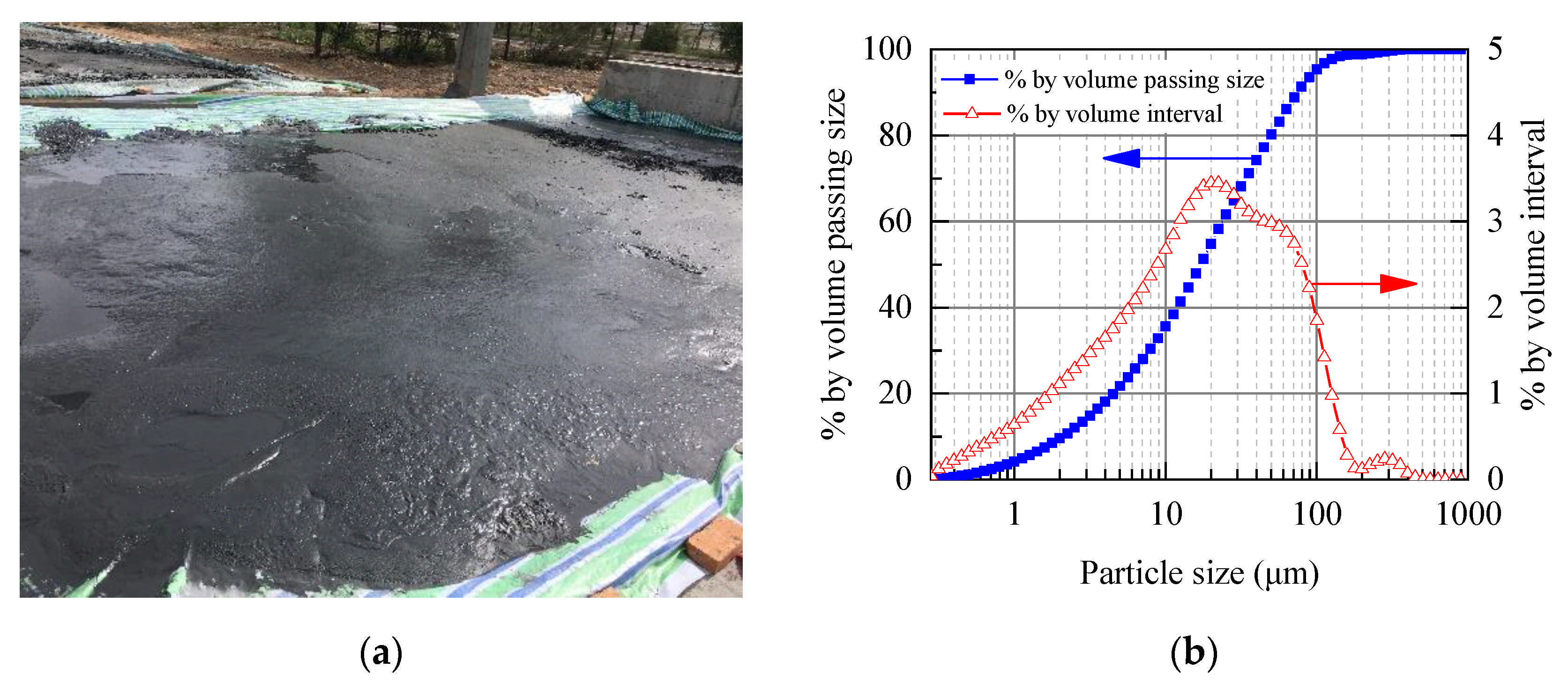
The total tailings sampled from the Jinchuan Nickel Deposit in China and anionic polyacrylamide flocculant (Magnafloc 5250) obtained from Badische Anilin-und-Soda-Fabrik (BASF) were used. The specific gravity of dry total tailings determined using a pycnometer is 2.785 g cm−3. The total tailings sample and the particle size distribution (PSD) of the total tailings obtained in the previous work are shown in Figure 1 [25].
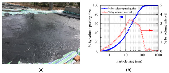
Figure 1.
Samples (a) and PSD (b) [25] of total tailings.
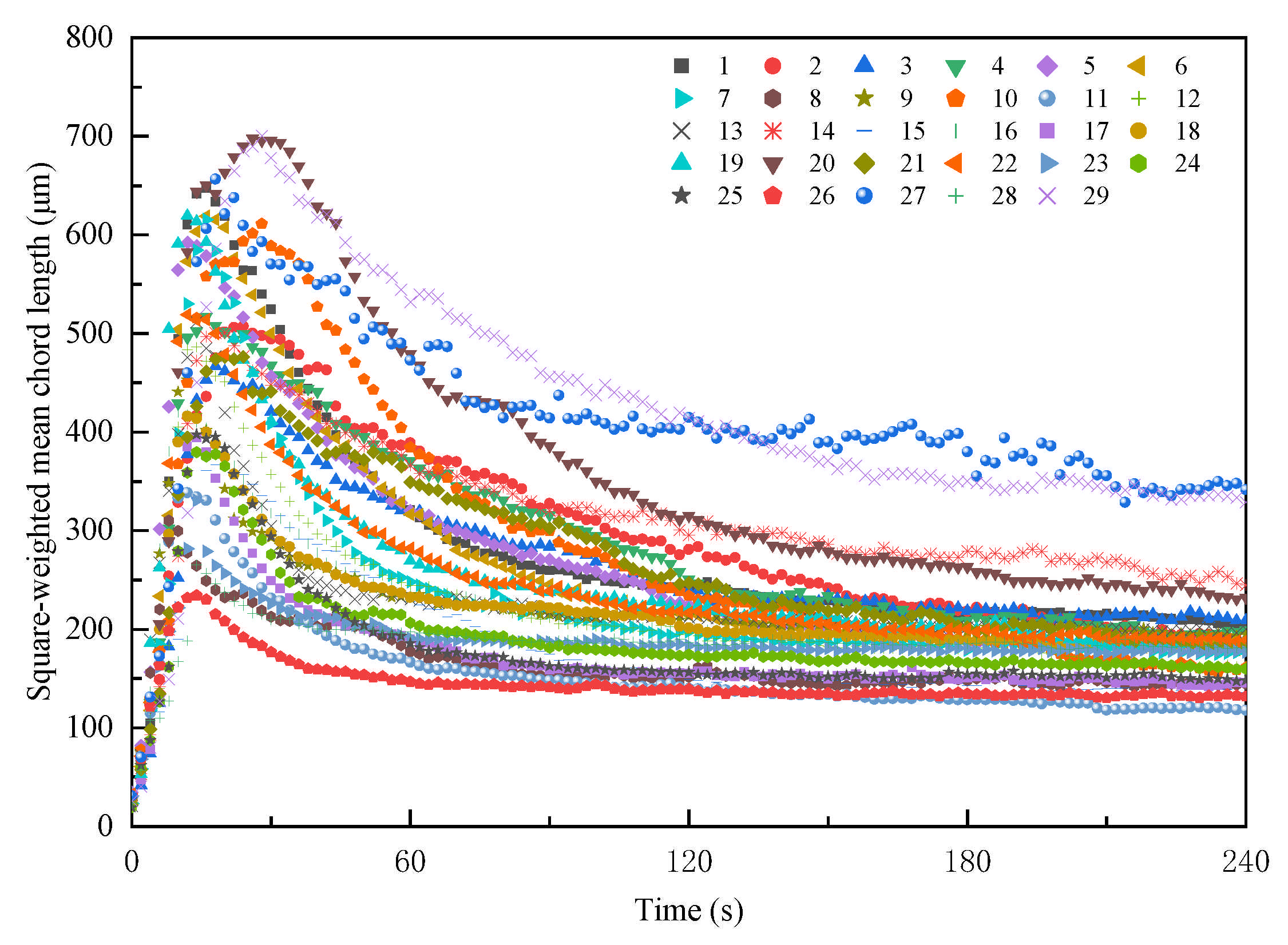
The solid fraction (SF), flocculant dosage (FD), flocculant concentration (FC), and shear rate (G) were selected as the factors. The ranges of the four factors are 5 wt% to 25 wt%, 5 g t−1 to 25 g t−1, 0.005% to 0.15%, and 51.60 s−1 to 412.90 s−1, respectively. About 29 experimental runs were designed by response surface methodology (RSM). The square-weighted mean chord length (SWMCL) of floc obtained by FBRM during the flocculation process was used to represent the floc size. The dynamic variation of the SWMCL of floc with flocculation time was shown in Figure 2 [25].
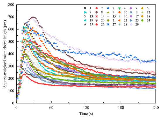
Figure 2.
Dynamic evolution of the square-weighted mean chord length of floc with flocculation time [25].
2.2. Population Balance Model (PBM)
PBM is very suitable for studying flocculation behavior [22,23]. In this work, we adopted the most popular expression for PBM, proposed by [26] and modified by [27], to describe the flocculation kinetics of total tailings. The aggregation kernel, breakage kernel, solution, and parameter fitting will be introduced in the following subsections.
where is the number concentration of flocs composed of particles at time t in channel i. N1 is the number concentration of primary particles in channel 1. The quantities and are collision frequency and collision efficiency, respectively. By , we denote breakage rate coefficient. Moreover, means a breakage distribution function. The superscripts and represent the maximum number of size channels used to describe the full-size range of particles and flocs, respectively, by aggregation and breakage. Values of and were determined in Section 3.1.
Each term on the right-hand side of Equation (1) represents the birth or death of flocs in channel I due to aggregation or breakage at time t. The first two terms describe the birth of flocs in the i-th channel due to the aggregation of smaller flocs. The next two terms represent the death of flocs in the i-th channel that aggregate to form larger flocs. The fifth term denotes the death of flocs in the i-th channel through breakage. The last term accounts for the birth of flocs in the i-th channel by breakage of larger flocs.
2.2.1. Aggregation Kernel
The aggregation kernel is the product of collision frequency and collision efficiency .
(1) Collision frequency.
The interparticle collision mechanism between particles is mainly related to the size of particles. For particles with diameters less than 1 μm, Brownian motion or perikinetic dominates; for particles in the diameter range 1 to 40 μm, fluid shear or orthokinetic dominates; and for particles with diameter larger than 40 μm, differential settling dominates [28]. As analyzed previously, the diameter range of total tailings particles is 0.282 to 447.744 μm, with 4.14% of which is less than 1 μm, 70.11% of which is in the range 1 to 40 μm, and 25.75% of which is larger than 40 μm [25]. Therefore, the collision between total-tailings flocs or particles results from the combined effects of Brownian motions, shear flow, and differential sedimentation. Thus, the collision frequency can be determined as:
where , , and are the collision frequency due to the three collision mechanisms, respectively.
Flocs were regarded as solid spheres in conventional models, which is seriously inconsistent with the facts. The flocs are porous and irregular, which can be described using fractal scaling [29]. Precisely, we assume that the floc size (gyration radius, ) is related to the number of primary particles () in a floc.
where is the radius of primary particle, is the mass fractal dimension, is a constant usually close to unity [30]. Experimental research investigated that the fractal dimension of flocs in the flocculation process of the same mineral particles is roughly constant, and the fractal dimension of flocs of different mineral particles is expected in the range of 1.8 to 2.8 [6,31,32]. In this work, 2.5 was assigned to the fractal dimension.
The permeability and fractal dimension of flocs should be considered to calculate the collision frequency due to the three mechanisms [33]:
where is the Boltzman constant, is the absolute temperature, and is the dynamic viscosity of the flocculating suspension:
where is the viscosity of water; is the maximum solid volume fraction. The porosity of total tailings in the dense state obtained by the experiment is 45.17%. When the pores of total tailings are filled with water, the volume fraction of total tailings is the largest. Therefore, the maximum solid volume fraction is 54.83%, which is 1 minus 45.17%. is the volume fraction of flocs, which is in relation to the average diameter of flocs and primary particles [32].
where is the volume fraction of primary particles in suspension.
In Equation (4), is the ratio between the force exerted by the fluid in a permeable floc and that on an impermeable sphere [34]:
where is a dimensionless factor of permeability,
where K represents the permeability, which can be calculated based on porosity, , through the Brinkman model [35],
where can be calculated based on and [36],
In Equation (5), and is the fluid collection efficiency and the average shear rate in the vessel [37], respectively:
where
Based on the modified Stokes law, in Equation (6) representing the sedimentation rate of permeable floc can be given as [22]:
where is the acceleration of gravity, and are the density of solid and water, respectively.
(2) Collision efficiency.
The collision efficiency is assumed to be 1 in the classical Smoluchowski coagulation equation [38]; that is to say, all collisions are effective. Actually, not all the collisions can generate a new larger floc because of the hydrodynamic retardation and colloidal interactions or repulsion [39]. Moreover, flocs are porous. For this reason, a semi-empirical equation proposed in [30] was introduced to describe the collision efficiency, namely
where , , and are fitting parameters, represents the maximal value of , which belongs to [0, 1], influenced by flocculant dosage and other flocculation conditions. In other studies, is treated as a tuning parameter in [40] while and are considered as 0.1 [41,42]. However, Equation (17) indicates that changes significantly with , , and . Therefore, , , and should be fitted to describe the collision efficiency
2.2.2. Breakage Kernel
Because of fluid shear, the flocs are likely to be broken. Since there is no theory to predict floc size distribution due to breakage, two similar power-law breakage rate coefficient models were developed [43,44]:
According to Equation (18), the breakage rate coefficient is related to shear rate and floc size. Based on this, we improved the model as another shear-induced power-law model:
where , , and are fitting parameters larger than 0.
Apart from the conditions for floc being broken, how the mass distribution of daughter flocs is also essential for describing the breakage process. Without any fitting or adjustable parameters, the binary breakage distribution function [45] was applied in this work. This model is easy to implement and the most used. It is simply defined as:
where and are the volume of flocs and , in which is the volume of the primary particle. The primary particle represents the basic unit of large particles or flocs [22,45]. And can be calculated based on the minimum size of total tailings particles.
2.3. PBM Solution and Parameter Fitting Methodology
As shown in Equation (1), PBM is a first-order linear ordinary differential equation (ODE). A stiff ODEs solver with low to medium accuracy (ode15s) in MATLAB was applied to solve the PBM. The fitting parameters in PBM were adjusted to the experimental data obtained from FBRM. To this end, we used particle swarm global optimization (PSO) to solve the following problem:
where is the De Brouckere Mean Diameter of flocs obtained from PBM, which can be calculated as follows; is the mean diameter of flocs obtained from FBRM measurement.
The Goodness of Fit [46] is used to validate model fit.
where , the closer the is to 1, the better fit of the PBM.
3. Results and Discussion
3.1. Initial Population of Total Tailings Particles
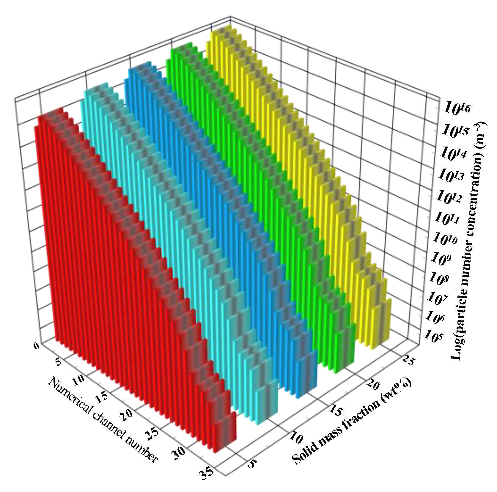
To solve Equation (1), we need the initial population of total tailings particles before flocculation. According to the previous studies [25,47], the minimum size of total tailings particles and the maximum size of total-tailings flocs are 0.282 μm and 1000 μm, respectively. Therefore, the volume of the primary particle is 1.17 × 10⁻²⁰ m3. At the same time, the largest volume of flocs is 5.23 × 10⁻¹⁰ m3, which is about 236.37−1 times of . Accordingly, we divided the size range of particles and flocs into 37 numerical channels. That is to say, both and in Equation (1) are 37. In the 29 experimental runs, there are five solid fractions (SFs), 5 wt%, 10 wt%, 15 wt%, 20 wt%, and 25 wt%. Based on the volume-based PSD (Figure 1b) and the SFs, the corresponding initial population of total tailings particles, that is, the number concentration distribution (m−3) of primary total tailings particles, can be calculated as shown in Figure 3. Because the PSDs of total tailings are the same under deferent SFs, the proportion of the same channel under deferent SFs is the same. At the same time, high SF means a high number concentration.

Figure 3.
Number concentration distribution of primary total tailings particles assigned in 37 channels.
3.2. Fitting the Parameters of PBM
The parameters , …, of the PBM of 29 experiment runs can be obtained as shown in Table 1.

Table 1.
Fitted parameters and statistics for each experiment run.
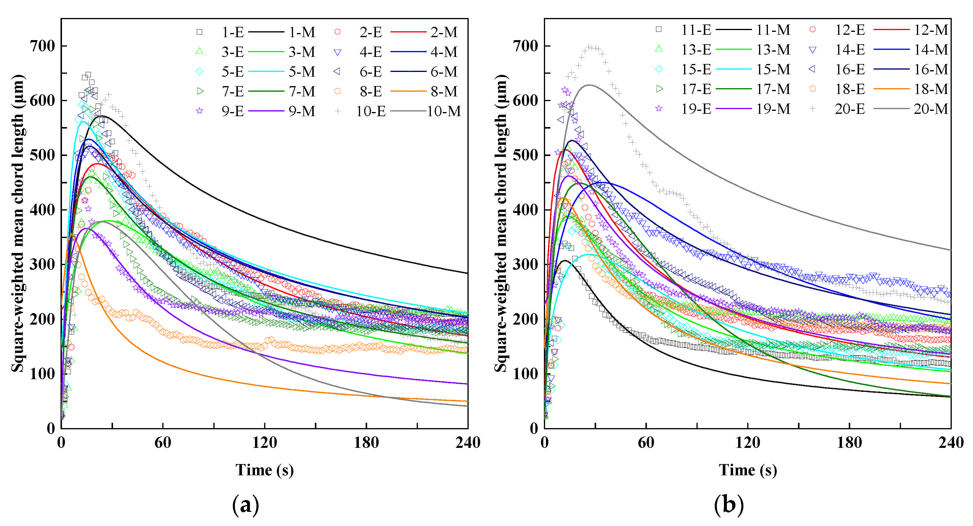
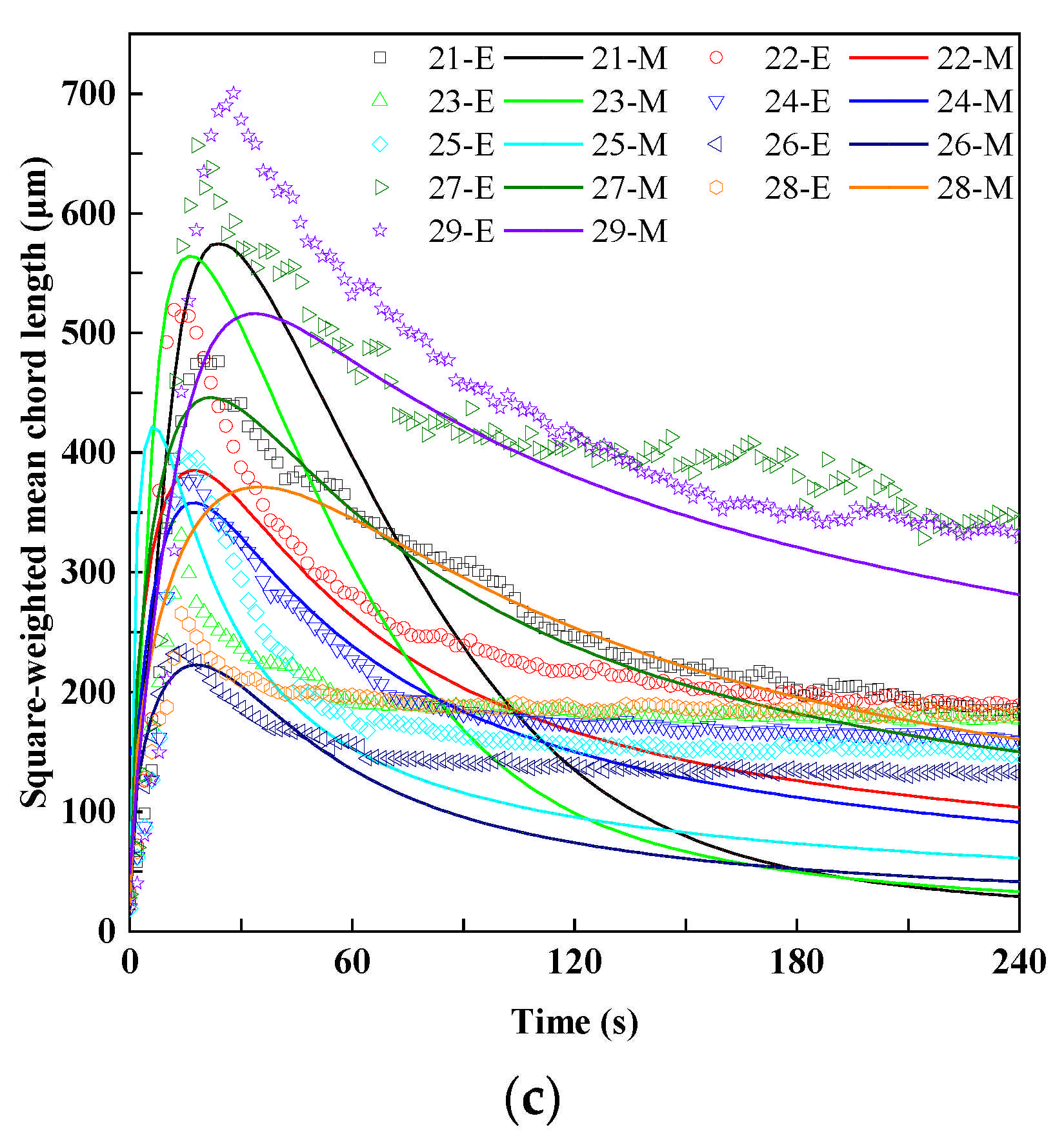
Substituting the value of , , and into Equation (17), covering the value of , , and into Equation (19), and solving Equation (1), we can obtain the dynamic evolution of the square-weighted mean chord length of floc in the corresponding experiment run. Figure 4 compares the dynamic evolution obtained by experiment and that obtained by modeling. It illustrates that PBM fit the experiment results well under most flocculation conditions. This result is confirmed by the values of shown in Table 1. The Goodness of Fit obtained through Equation (24) is close to 1 in most runs.
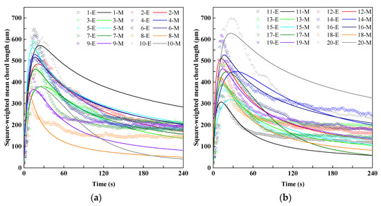
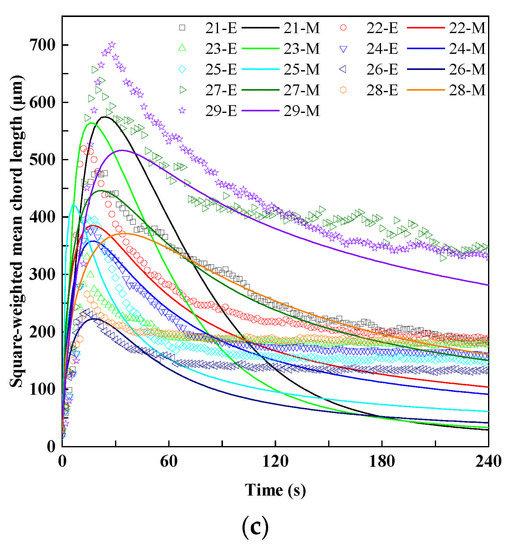
Figure 4.
Dynamic evolution of the square-weighted mean chord length of floc obtained by experiment (symbols) and modeling (continuous lines) in (a) run 1 to 10; (b) run 11 to 20, and (c) run 21 to 29. In the legend, E and M represent experiment and modeling, respectively.
3.3. Analysis of the Parameters
It can be seen from Table 1 that of the PBM of 29 experiment runs was close to 1, and the average is 0.888772. That is to say, the maximal value of the collision efficiency () is smaller than 1, which is always adopted in the classical Smoluchowski coagulation equation [38]. The average of and are 0.904795 and 0.022526, respectively. Both and are not 0.1 as considered in other studies [41,42]. Moreover, neither nor is 1, indicating that the breakage rate coefficient of total-tailings flocs is not in line with the shear rate or floc size. At the same time, it also illustrates that the breakage rate coefficient of total-tailings flocs is different from that of other flocs or droplets [43,44].
The of run 16 and 20 in Table 1 are the two largest among all the experiment runs. Therefore, we take run 16 and 20 as examples to analyze the evolution of collision efficiency with the numerical channel I and j. The collision efficiencies estimated using the corresponding values of , , and in run 16 and run 20 are shown in Figure 5. Both Figure 5a,b illustrate higher values for smaller flocs that are comparable in size.
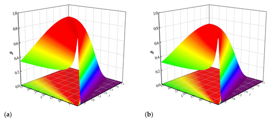
Figure 5.
Collision efficiency in PBM of (a) run 16; (b) run 20. The x-axis and y-axis represent the numerical channel I and j, respectively. The z-axis denotes collision efficiency .
The exponent () of shear rate (G) in shear-induced breakage rate coefficient fluctuates around 1. The average of is 0.991630. This result is similar to the exponent of G in Equation (19). Therefore, the breakage rate coefficient is approximately positive linear with G for the flocs of the same size. The exponent () of floc size () fluctuates around 2. The average of is 1.824650. Therefore, the breakage rate coefficient is approximately positive linear with the square of under the same shear condition. The parameter is significantly less than and , respectively. The average of is 0.059563.
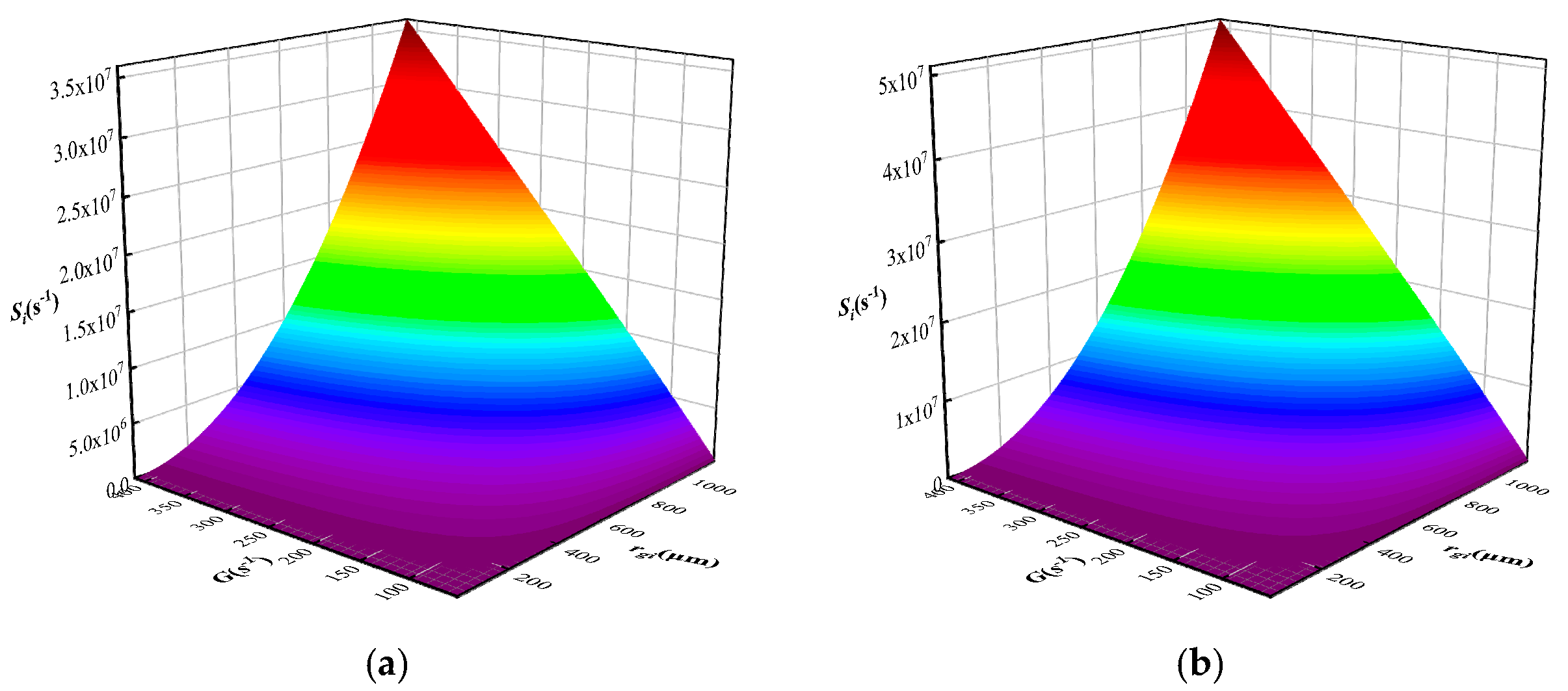
We also take run 16 and 20 as examples to analyze the changes of breakage rate coefficient with the shear rate and gyration radius . The breakage rate coefficients estimated using the corresponding values of , , and in run 16 and run 20 are shown in Figure 6. Both Figure 6a,b demonstrate higher values for higher shear rate and bigger gyration radius.
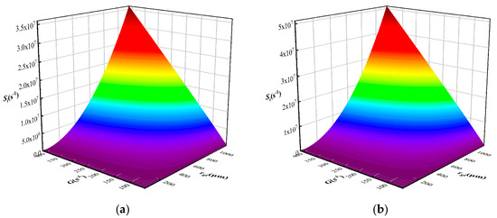
Figure 6.
Breakage rate coefficient in PBM of (a) run 16; (b) run 20. The x-axis and y-axis represent the shear rate and gyration radius , respectively. The z-axis denotes the breakage rate coefficient .
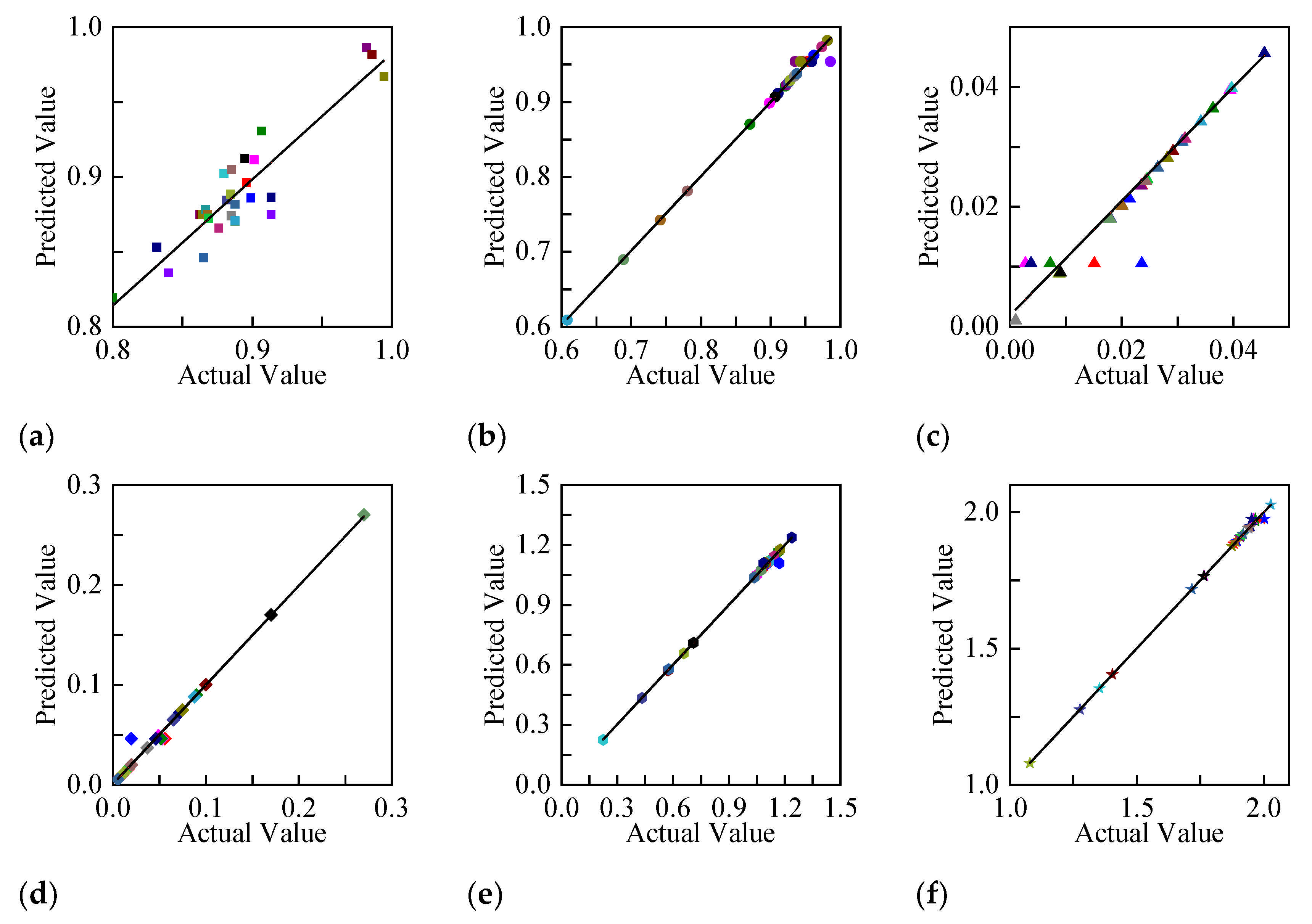
Moreover, , …, of the PBM of each experiment run is quite different from that of other runs, indicating that all of the six fitting parameters vary with flocculation conditions. Therefore, the fitting parameters are functions of flocculation factors. The regression processes were conducted through Design-Expert software. Before regression, the factor should be coded as −1 to 1 because of the difference between the unit and/or level of each factor [25]. The regression models obtained for , …, in terms of coded factors were obtained, as shown in Equations (25)–(30), respectively.
The coefficient of determination of the regression models were 0.8415, 0.9928, 0.9152, 0.9926, 0.9971, and 0.9989, respectively. This result is confirmed by Figure 7, in which the plots of predicted , …, versus actual ones are shown. Therefore, Equations (25)–(30) fit the calculated results well and are capable of sufficient predicting , …, under the given experimental setup, respectively.
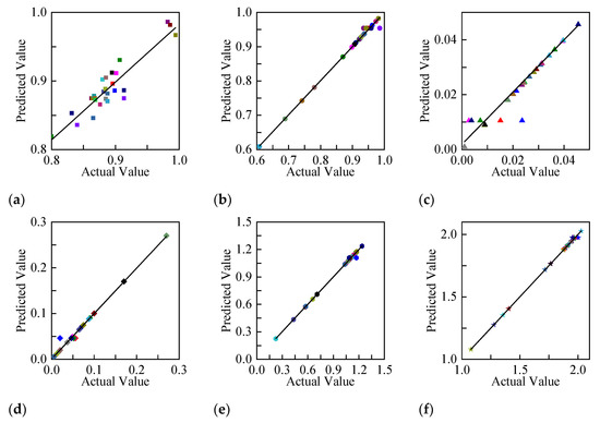
Figure 7.
Predicted vs. actual values plot for responses: (a) ; (b) ; (c) ; (d) ; (e) ; and (f) .
3.4. Validation of PBM
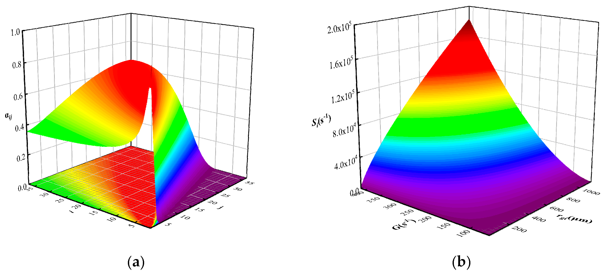
To further test the validity of PBM and the regression models, we used the experiment results obtained under the optimal flocculation conditions in a previous study [25] to conduct the validation. The optimal flocculation conditions were SF = 10.29%, FD = 25%, FC = 0.15%, and G = 51.60 s−1. Correspondingly, the fitting parameters , …, were 0.93340, 0.83532, 0.04749, 0.11752, 0.76734, and 1.65428, respectively. The corresponding collision efficiency and breakage rate coefficient estimated are shown in Figure 8. It can be found from Figure 8b that the breakage rate coefficient is much lower than that of run 16 and run 20 (Figure 6), indicating that the flocs are not easy to break under the optimal conditions.
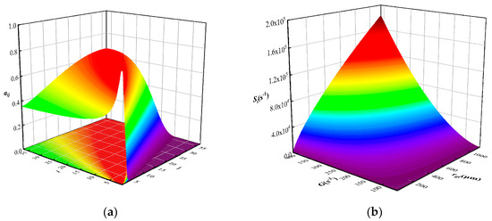
Figure 8.
(a) Collision efficiency and (b) breakage rate coefficient in PBM under the optimal conditions.
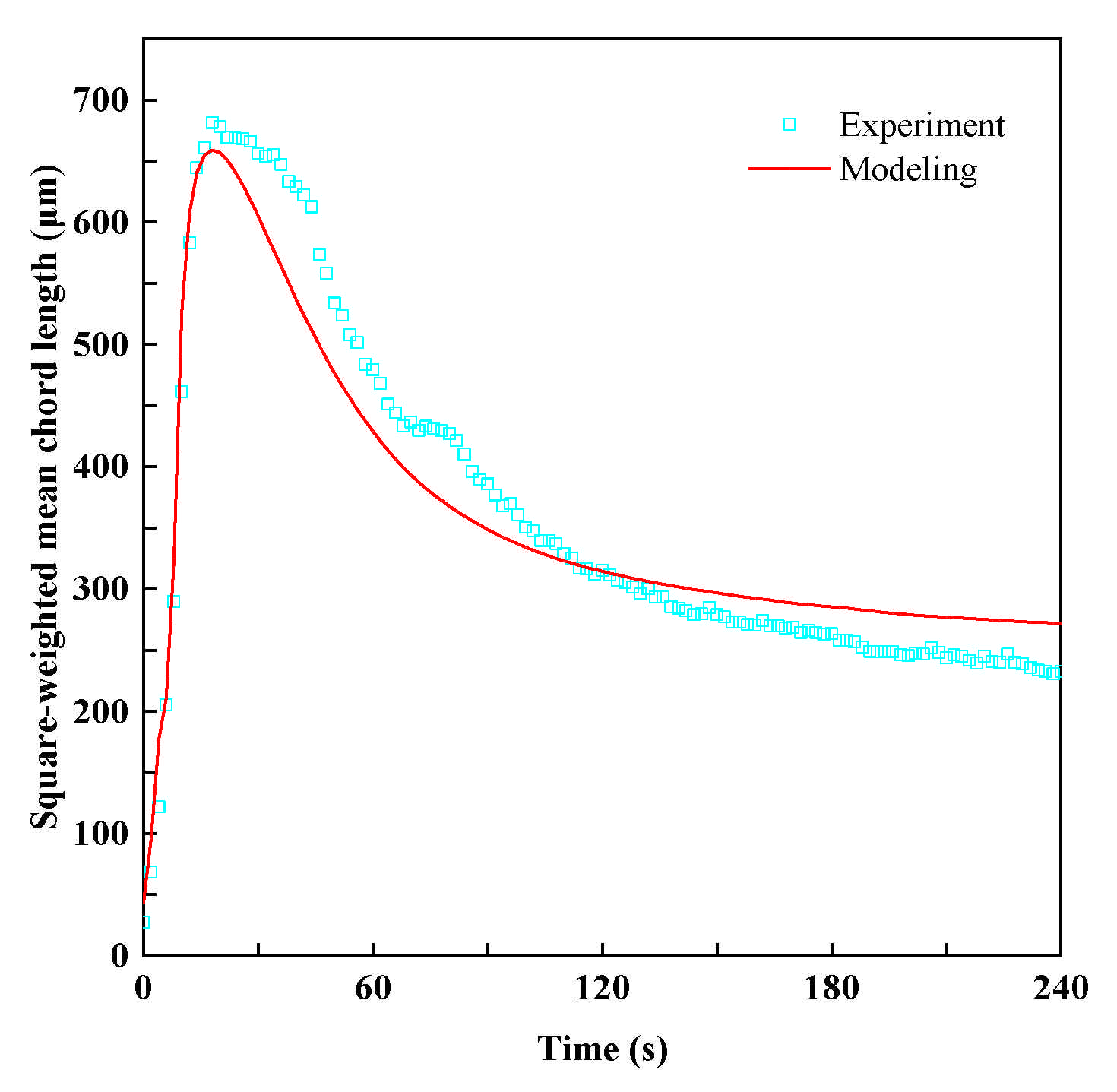
The dynamic evolution of the square-weighted mean chord length of floc obtained by modeling under the optimal conditions can be obtained, as shown in Figure 9.
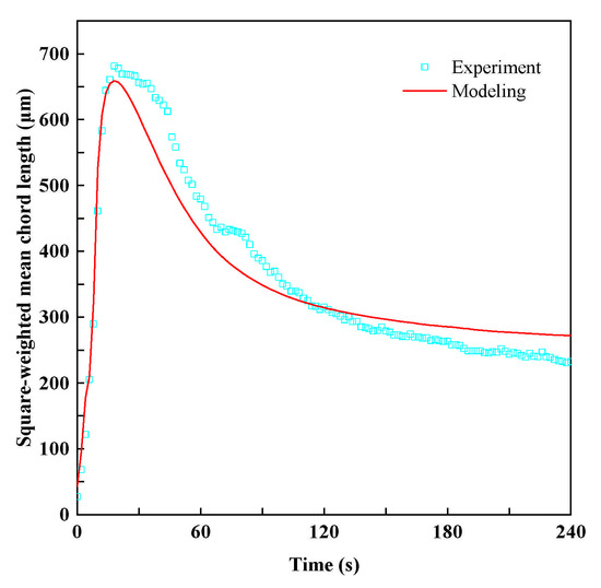
Figure 9.
Dynamic evolution of the square-weighted mean chord length of floc obtained by experiment (symbols) and modeling (continuous lines) under the optimal conditions.
Because the fitting parameters of PBM are determined based on the experiment database (results of 29 experimental runs designed RSM), the PBM can predicate the flocculation under different flocculation conditions. The modeling results are close to the experiment results. The coefficient of determination between modeling and experiment is 0.9804. This result further proves that the regression models for , …, are valid. That is to say, the proposed PBM quantifies well the dynamic evolution of the floc size during flocculation under the given experimental setup. Moreover, it is reasonable to expect that if the experiment database is large enough, the prediction accuracy of the PBM will be more be higher.
Therefore, we can predict the particle or floc size distribution during flocculation using the proposed PBM under the given experimental setup. Furthermore, we can model the total-tailings floc size evolution in the feedwells of thickener by coupling CFD with PBM.
4. Conclusions
This work proposed a flocculation kinetics model based on PBM to model the polymer-bridging flocculation process of total tailings. In the aggregation kernel, a collision frequency model is used to describe the particle collision under the combined effects of Brownian motions, shear flow, and differential sedimentation. A semi-empirical collision efficiency model with three fitting parameters (, , and ) was applied. A shear-induced power-law breakage rate coefficient model with another three fitting parameters (, , and ) was introduced in the breakage kernel. The breakage rate coefficient is related to shear rate and floc size.
A solver from Matlab (ode15s) was applied to solve the PBM. Values of the six fitting parameters were determined by minimizing the difference between experimental data and modeling results. The six fitting parameters vary with flocculation conditions, and the average of , …, are 0.888772, 0.904795, 0.022526, 0.059563, 0.991630, 1.824650, respectively. The six fitting parameters were regressed with the flocculation factors. The regression models for , …, in terms of coded factors were obtained. The validation modeling demonstrated that the proposed PBM quantifies well the dynamic evolution of the floc size during flocculation under the given experimental setup.
The PBM proposed is suitable for the Magnafloc 5250 and total tailings in Jinchuan Nickel Deposit. The investigation will provide significant new insights into the flocculation kinetics of total tailings and lay a foundation for studying the performance of the feedwell of a gravity thickener. In the future, we will try to fit the six fitting parameters to describe the shear-induced polymer-bridging flocculation of other tailings, such as copper tailings and iron tailings. Besides, other flocculation factors ignored in this work should be considered to improve the validity of PBM. Moreover, the evolution of size and that of fractal dimension of flocs should be considered simultaneously.
Author Contributions
Conceptualization, Z.R. and A.W.; methodology, Z.R., R.B., F.B. and J.W.; software, Z.R. and R.O.; validation, Z.R. and J.W.; formal analysis, Z.R. and S.W.; investigation, Z.R.; resources, A.W.; data curation, Z.R.; writing—original draft preparation, Z.R.; writing—review and editing, A.W., R.B., F.B. and Y.W.; supervision, A.W., R.B. and F.B.; project administration, A.W.; funding acquisition, Z.R., A.W., R.B., F.B., S.W. and Y.W. All authors have read and agreed to the published version of the manuscript.
Funding
This research was funded by the National Natural Science Foundation of China (No. 52130404, 51774039, 51804015); China Postdoctoral Science Foundation (No. 2021M690011); Beijing Municipal Natural Science Foundation (No. 8192029); Postdoctor Research Foundation of Shunde Graduate School of University of Science and Technology Beijing (No. 2021BH011); ANID (Chile) through Fondecyt project 1210610; Centro de Modelamiento Matemático (BASAL funds for Centers of Excellence ACE 210010 and FB210005); CRHIAM, project ANID/FONDAP/15130015; and Anillo project ANID/PIA/ACT210030.
Data Availability Statement
Data available on request due to restrictions.
Acknowledgments
The authors acknowledge Jinchuan Group Ltd. and BASF for providing the materials; Jiaqing Chen and Xiaolei Cai for providing FBRM and guiding in the experiment; and Wenjia Dai for guiding the MATLAB code.
Conflicts of Interest
The authors declare no conflict of interest.
References
- Santamarina, J.C.; Torres-Cruz, L.A.; Bachus, R.C. Why coal ash and tailings dam disasters occur. Science 2019, 364, 526–528. [Google Scholar] [CrossRef]
- Silva Rotta, L.H.; Alcântara, E.; Park, E.; Negri, R.G.; Lin, Y.N.; Bernardo, N.; Mendes, T.S.G.; Souza Filho, C.R. The 2019 Brumadinho tailings dam collapse: Possible cause and impacts of the worst human and environmental disaster in Brazil. Int. J. Appl. Earth Obs. Geoinf. 2020, 90, 102119. [Google Scholar] [CrossRef]
- Wang, C.; Harbottle, D.; Liu, Q.; Xu, Z. Current state of fine mineral tailings treatment: A critical review on theory and practice. Miner. Eng. 2014, 58, 113–131. [Google Scholar] [CrossRef]
- Qi, C.; Fourie, A. Cemented paste backfill for mineral tailings management: Review and future perspectives. Miner. Eng. 2019, 144, 106025. [Google Scholar] [CrossRef]
- Chen, X.; Jin, X.; Jiao, H.; Yang, Y.; Liu, J. Pore connectivity and dewatering mechanism of tailings bed in raking deep-cone thickener process. Minerals 2020, 10, 375. [Google Scholar] [CrossRef]
- Grabsch, A.F.; Fawell, P.D.; Adkins, S.J.; Beveridge, A. The impact of achieving a higher aggregate density on polymer-bridging flocculation. Int. J. Miner. Process. 2013, 124, 83–94. [Google Scholar] [CrossRef]
- Fawell, P.D.; Nguyen, T.V.; Solnordal, C.B.; Stephens, D.W. Enhancing Gravity Thickener Feedwell Design and Operation for Optimal Flocculation through the Application of Computational Fluid Dynamics. Miner. Process. Extr. Metall. Rev. 2019, 42, 496–510. [Google Scholar] [CrossRef]
- Ruan, Z.; Wu, A.; Bürger, R.; Betancourt, F.; Wang, Y.; Wang, Y.; Jiao, H.; Wang, S. Effect of interparticle interactions on the yield stress of thickened flocculated copper mineral tailings slurry. Powder Technol. 2021, 392, 278–285. [Google Scholar] [CrossRef]
- Qi, C.; Fourie, A.; Chen, Q.; Tang, X.; Zhang, Q.; Gao, R. Data-driven modelling of the flocculation process on mineral processing tailings treatment. J. Clean. Prod. 2018, 196, 505–516. [Google Scholar] [CrossRef]
- Jiao, H.; Wang, S.; Yang, Y.; Chen, X. Water recovery improvement by shearing of gravity-thickened tailings for cemented paste backfill. J. Clean. Prod. 2020, 245, 118882. [Google Scholar] [CrossRef]
- Jiao, H.; Wu, Y.; Wang, H.; Chen, X.; Li, Z.; Wang, Y.; Zhang, B.; Liu, J. Micro-scale mechanism of sealed water seepage and thickening from tailings bed in rake shearing thickener. Miner. Eng. 2021, 173, 107043. [Google Scholar] [CrossRef]
- Betancourt, F.; Celi, D.; Cornejo, P.; del Río, M.; Macera, L.; Pereira, A.; Rulyov, N. Comparison of ultra-flocculation reactors applied to fine quartz slurries. Miner. Eng. 2020, 148, 106074. [Google Scholar] [CrossRef]
- Hornn, V.; Park, I.; Ito, M.; Shimada, H.; Suto, T.; Tabelin, C.B.; Jeon, S.; Hiroyoshi, N. Agglomeration-flotation of finely ground chalcopyrite using surfactant-stabilized oil emulsions: Effects of co-existing minerals and ions. Miner. Eng. 2021, 171, 107076. [Google Scholar] [CrossRef]
- Hornn, V.; Ito, M.; Shimada, H.; Tabelin, C.B.; Jeon, S.; Park, I.; Hiroyoshi, N. Agglomeration–Flotation of Finely Ground Chalcopyrite Using Emulsified Oil Stabilized by Emulsifiers: Implications for Porphyry Copper Ore Flotation. Metals 2020, 10, 912. [Google Scholar] [CrossRef]
- Hornn, V.; Ito, M.; Yamazawa, R.; Shimada, H.; Tabelin, C.B.; Jeon, S.; Park, I.; Hiroyoshi, N. Kinetic Analysis for Agglomeration-Flotation of Finely Ground Chalcopyrite: Comparison of First Order Kinetic Model and Experimental Results. Mater. Trans. 2020, 61, 1940–1948. [Google Scholar] [CrossRef]
- Hornn, V.; Ito, M.; Shimada, H.; Tabelin, C.B.; Jeon, S.; Park, I.; Hiroyoshi, N. Agglomeration-Flotation of Finely Ground Chalcopyrite and Quartz: Effects of Agitation Strength during Agglomeration Using Emulsified Oil on Chalcopyrite. Minerals 2020, 10, 380. [Google Scholar] [CrossRef]
- Concha, F.; Rulyov, N.N.; Laskowski, J.S. Settling velocities of particulate systems 18: Solid flux density determination by ultra-flocculation. Int. J. Miner. Process. 2012, 104–105, 53–57. [Google Scholar] [CrossRef]
- Senaputra, A.; Jones, F.; Fawell, P.D.; Smith, P.G. Focused beam reflectance measurement for monitoring the extent and efficiency of flocculation in mineral systems. AIChE J. 2014, 60, 251–265. [Google Scholar] [CrossRef]
- Sharma, S.; Lin, C.L.; Miller, J.D. Multi-scale features including water content of polymer induced kaolinite floc structures. Miner. Eng. 2017, 101, 20–29. [Google Scholar] [CrossRef] [Green Version]
- Elfarissi, F.; Pefferkorn, E. Fragmentation of Kaolinite Aggregates Induced by Ion-Exchange Reactions within Adsorbed Humic Acid Layers. J. Colloid Interface Sci. 2000, 221, 64–74. [Google Scholar] [CrossRef]
- Odriozola, G.; Schmitt, A.; Moncho-Jordá, A.; Callejas-Fernández, J.; Martínez-García, R.; Leone, R.; Hidalgo-Álvarez, R. Constant bond breakup probability model for reversible aggregation processes. Phys. Rev. E 2002, 65, 031405. [Google Scholar] [CrossRef] [PubMed] [Green Version]
- Jeldres, R.I.; Fawell, P.D.; Florio, B.J. Population balance modelling to describe the particle aggregation process: A review. Powder Technol. 2018, 326, 190–207. [Google Scholar] [CrossRef]
- Quezada, G.R.; Jeldres, M.; Robles, P.; Toro, N.; Torres, D.; Jeldres, R.I. Improving the Flocculation Performance of Clay-Based Tailings in Seawater: A Population Balance Modelling Approach. Minerals 2020, 10, 782. [Google Scholar] [CrossRef]
- Tanguay, M.; Fawell, P.; Adkins, S. Modelling the impact of two different flocculants on the performance of a thickener feedwell. Appl. Math. Model. 2014, 38, 4262–4276. [Google Scholar] [CrossRef]
- Wu, A.; Ruan, Z.; Bürger, R.; Yin, S.; Wang, J.; Wang, Y. Optimization of flocculation and settling parameters of tailings slurry by response surface methodology. Miner. Eng. 2020, 156, 106488. [Google Scholar] [CrossRef]
- Hounslow, M.J.; Ryall, R.L.; Marshall, V.R. A discretized population balance for nucleation, growth, and aggregation. AIChE J. 1988, 34, 1821–1832. [Google Scholar] [CrossRef]
- Spicer, P.T.; Pratsinis, S.E. Coagulation and Fragmentation: Universal Steady-State Particle-Size Distribution. AIChE J. 1996, 42, 1612–1620. [Google Scholar] [CrossRef]
- Oyegbile, B.; Ay, P.; Narra, S. Flocculation kinetics and hydrodynamic interactions in natural and engineered flow systems: A review. Environ. Eng. Res. 2016, 21, 1–14. [Google Scholar] [CrossRef] [Green Version]
- Mandelbrot, B.B. Self-affine fractals and fractal dimension. Phys. Scr. 1985, 32, 257–260. [Google Scholar] [CrossRef]
- Kusters, K.A.; Wijers, J.G.; Thoenes, D. Aggregation kinetics of small particles in agitated vessels. Chem. Eng. Sci. 1997, 52, 107–121. [Google Scholar] [CrossRef] [Green Version]
- Quezada, G.R.; Ramos, J.; Jeldres, R.I.; Robles, P.; Toledo, P.G. Analysis of the flocculation process of fine tailings particles in saltwater through a population balance model. Sep. Purif. Technol. 2020, 237, 116319. [Google Scholar] [CrossRef]
- Heath, A.R.; Bahri, P.A.; Fawell, P.D.; Farrow, J.B. Polymer flocculation of calcite: Population balance model. AIChE J. 2006, 52, 1641–1653. [Google Scholar] [CrossRef]
- Veerapaneni, S.; Wiesner, M.R. Hydrodynamics of fractal aggregates with radially varying permeability. J. Colloid Interface Sci. 1996, 177, 45–57. [Google Scholar] [CrossRef]
- Neale, G.; Epstein, N.; Nader, W. Creeping flow relative to permeable spheres. Chem. Eng. Sci. 1973, 28, 1865–1874. [Google Scholar] [CrossRef]
- Li, X.Y.; Logan, B.E. Permeability of fractal aggregates. Water Res. 2001, 35, 3373–3380. [Google Scholar] [CrossRef]
- Vainshtein, P.; Shapiro, M.; Gutfinger, C. Mobility of permeable aggregates: Effects of shape and porosity. J. Aerosol Sci. 2004, 35, 383–404. [Google Scholar] [CrossRef]
- Camp, T.R.; Stein, P.C. Velocity Gradients and Internal Work in Fluid Motion. J. Bost. Soc. Civ. Eng. 1943, 30, 219–237. [Google Scholar]
- Smoluchowski, M.V. Versuch einer mathematischen Theorie der Koagulationskinetik kolloider Lösungen. Z. Phys. Chem. 1918, 92U, 129–168. [Google Scholar] [CrossRef] [Green Version]
- Adler, P. Heterocoagulation in shear flow. J. Colloid Interface Sci. 1981, 83, 106–115. [Google Scholar] [CrossRef]
- Soos, M.; Sefcik, J.; Morbidelli, M. Investigation of aggregation, breakage and restructuring kinetics of colloidal dispersions in turbulent flows by population balance modeling and static light scattering. Chem. Eng. Sci. 2006, 61, 2349–2363. [Google Scholar] [CrossRef]
- Selomulya, C.; Bushell, G.; Amal, R.; Waite, T.D. Understanding the role of restructuring in flocculation: The application of a population balance model. Chem. Eng. Sci. 2003, 58, 327–338. [Google Scholar] [CrossRef]
- Antunes, E.; Garcia, F.A.P.; Ferreira, P.; Blanco, A.; Negro, C.; Rasteiro, M.G. Modelling PCC flocculation by bridging mechanism using population balances: Effect of polymer characteristics on flocculation. Chem. Eng. Sci. 2010, 65, 3798–3807. [Google Scholar] [CrossRef]
- Pandya, J.D.; Spielman, L.A. Floc breakage in agitated suspensions: Theory and data processing strategy. J. Colloid Interface Sci. 1982, 90, 517–531. [Google Scholar] [CrossRef]
- Pandya, J.D.; Spielman, L.A. Floc breakage in agitated suspensions: Effect of agitation rate. Chem. Eng. Sci. 1983, 38, 1983–1992. [Google Scholar] [CrossRef]
- Chen, W.; Fischer, R.R.; Berg, J.C. Simulation of particle size distribution in an aggregation-breakup process. Chem. Eng. Sci. 1990, 45, 3003–3006. [Google Scholar] [CrossRef]
- Asuero, A.G.; Sayago, A.; González, A.G. The Correlation Coefficient: An Overview. Crit. Rev. Anal. Chem. 2006, 36, 41–59. [Google Scholar] [CrossRef]
- Ruan, Z.; Wu, A.; Wang, J.; Yin, S.; Wang, Y. Flocculation and settling behavior of unclassified tailings based on measurement of floc chord length. Chin. J. Eng. 2020, 42, 980–987. [Google Scholar] [CrossRef]

Publisher’s Note: MDPI stays neutral with regard to jurisdictional claims in published maps and institutional affiliations. |
© 2021 by the authors. Licensee MDPI, Basel, Switzerland. This article is an open access article distributed under the terms and conditions of the Creative Commons Attribution (CC BY) license (https://creativecommons.org/licenses/by/4.0/).