Abstract
Control systems require maintenance in the form of tuning their parameters in order to maximize their performance in the face of process changes in minerals processing circuits. This work focuses on using deep reinforcement learning to train an agent to perform this maintenance continuously. A generic simulation of a first-order process with a time delay, controlled by a proportional-integral controller, was used as the training environment. Domain randomization in this environment was used to aid in generalizing the agent to unseen conditions on a physical circuit. Proximal policy optimization was used to train the agent, and hyper-parameter optimization was performed to select the optimal agent neural network size and training algorithm parameters. Two agents were tested, examining the impact of the observation space used by the agent and concluding that the best observation consists of the parameters of an auto-regressive with exogenous input model fitted to the measurements of the controlled variable. The best trained agent was deployed at an industrial comminution circuit where it was tested on two flow rate control loops. This agent improved the performance of one of these control loops but decreased the performance of the other control loop. While deep reinforcement learning does show promise in controller tuning, several challenges and directions for further study have been identified.
1. Introduction
Reinforcement learning (RL) is concerned with training an autonomous agent to interact with an environment to achieve a target goal, such as tuning a proportional-integral (PI) controller to maximize performance. Recent progress combining deep neural networks with RL, called deep RL (DRL), has led to successes in challenging robotics problems [1,2,3,4], as well as achieving superhuman performance in some games [5,6]. Further details regarding RL fundamentals can be found in the textbook by Sutton and Barto [7].
The work reported in this article examines whether it is possible to train a DRL agent to tune a range of proportional-integral (PI) controllers. These controllers are commonly used in minerals processing circuits as low-level controllers upon which higher-level optimizing controllers depend. PI and proportional-integral-derivative (PID) controllers constitute the majority of control systems encountered in industrial applications [8,9]. However, finding suitable methods for tuning these controllers automatically is still a subject of research. Tuning formulae exist for PI controllers for first-order systems [10,11,12], which may be suitable when the gain, time delay, and time constant of the system are known. However, this is seldom the case. Other tuning methods include heuristics, such as the Ziegler–Nichols method, frequency response methods, optimization methods, and adaptive tuning methods [13]. RL algorithms have been formulated for PID controller tuning, where the PID controller is viewed as the policy function in the agent [14,15,16]; hence, the training process directly updates the controller parameters. As an example, Lu et al. [14] and Xiu et al. [15] use an algorithm that views the PID controller as a basic neural network and updates the weights, i.e., the controller gains, in real time using supervised Hebb learning. This method retains a global gain parameter that must be adjusted via another method, e.g., fuzzy rules [15], which is specific to the process under control and hence incompatible with the goal of creating a general PI controller tuning agent. Model-based RL has been used to tune multiple PID controllers simultaneously in a multi-input, multi-output robotic system [16]. Here, the learned model is used to estimate the future performance of the controller parameters. An optimization loop, similar to receding horizon control, selects the optimal controller parameters.
Traditional RL and DRL algorithms have been applied to PID controller tuning by treating the actions taken by the agent as controller gains or changes to these controller gains. Here, the training process does not directly set the controller gains, but rather updates a combination of value and policy functions. The policy function sets the controller gains based on the current state of the process under control. Actor–critic RL algorithms may be used to directly set controller gains from changes in the error signal, e.g., in robotics problems [17,18]. Discrete controller parameter values were used by El Hakim et al. [19], allowing them to use Q-learning to train an agent to perform the action of selecting one of a fixed number of combinations of controller gains. Discrete actions can take the form of incremental changes to the controller gains, e.g., by multiplying the gains by fixed constants [20]. Any RL algorithm can be applied in this scenario, wherein the action is to select one combination of controller gain changes from the set of possible incremental changes. The continuous state, e.g., determined from past and present tracking error values, can be discretized as well [19,20]. These algorithms, as well as those that treat the controller as the policy function, only learn to tune controllers on a single system or plant.
In contrast to the methods described above, the work presented here attempts to train a generic agent that is capable of tuning PI controllers for a range of plants. Once the agent has been trained and is deployed on a physical control loop, it adjusts the controller gains based on the current state of the control loop. No additional exploration is performed. Prior work by Shipman and Coetzee [21] demonstrated the training of a similar agent using a modified advantage actor–critic (A2C) algorithm, although this agent failed to generalize well to testing on a physical plant. In comparison, this work has significantly increased the complexity of the training simulation, uses proximal policy optimization (PPO) to train the agent, and includes hyper-parameter optimization. Note that the rewards cannot be compared between this work and the prior work by Shipman and Coetzee as the simulation complexity has increased, resulting in lower rewards in this work.
The remainder of this article is structured as follows: Section 2 describes the training methods used in this work, data preprocessing steps, and the industrial testing procedure. Section 3 documents the results of the tests conducted both in simulation and on a minerals processing plant. Section 4 discusses these results, concluding with remarks on possible future improvements.
2. Materials and Methods
Figure 1 provides a high-level overview of the system used to train and optimize the agents in this work, showing the Markov decision process (the simulation, agent, observation, reward, and action), followed by the hyper-parameter optimization step. The simulation environment (Section 2.1) provides time series data and a reward. The time series data may be processed further by an observation method (Section 2.2) before being supplied to the agent as an observation of the underlying state of the system. The agent generates new controller gains for the PI controller and learns from the observations and rewards. This agent training process runs for a number of steps, followed by performing a test to assess the performance of the agent. This performance is used by a hyper-parameter optimizer (Section 2.3) that adjusts the hyper-parameters of the PPO algorithm to maximize the performance of the agent.
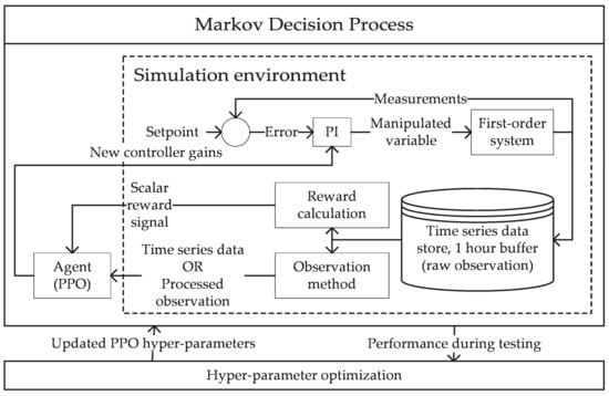
Figure 1.
Block diagram of the system showing the simulation environment, data processing, agent, and hyper-parameter optimization step.
2.1. Simulation Environment
The simulation environment models a first-order system with varying set points, manipulated variable (MV) disturbances, measurement noise, discrete MVs, and discrete controlled variables (CVs), controlled by a PI controller. The PI controller regulates the CV to a given set point variable (SV) value, which is derived from a fixed set of trajectory functions in this work. The gain, , time constant, , and time delay in seconds, , of the system were randomly varied in the ranges 1 to 15, 0.5 to 10, and 1 to 10, respectively. The gain of the controller, , and the integral time, , were constrained to the ranges 0.005 to 2 and 0.5 to 50, respectively. and are chosen by the RL agent to maximize the discounted future reward obtained from the environment, i.e., the overall performance of the closed-loop system. The outputs of the actor network of the RL agent ranged from to , owing to the use of the hyperbolic tangent (tanh) activation function on the output layer of the neural network. These outputs were scaled to the ranges shown above for and .
The discretized first-order model of the system, with sampling time seconds, is as follows:
The MV, , is constrained to the range , while the CV, , is constrained to the range . The CV consists of the state and pink noise with a randomly chosen scale factor drawn from a uniform random distribution with range multiplied by the SV offset. This SV offset is drawn from a uniform random distribution in the range . Further details on the derivation of these limits and the set of functions used to generate the SV are provided in Appendix A. In approximately 50 % of the training episodes, the MV is passed through a non-linearity, Equation (3), to simulate the effect of actuator non-linearities.
The MV is discretized in 75% of the simulations, with equal probability of the selected rounding mode being set to round up, round down, or round to the nearest integer. CV discretization is handled differently, by randomly selecting the number of discrete levels between integer measurements. The CV is then rounded to the nearest discrete value. In 20% of the episodes, the CV is not discretized, while in the remaining 80% of the episodes, it is discretized using 1, 2, 3, or 4 levels with equal probability. The discretization formula is , where is the number of discretization levels. The case of a continuous MV and CV with no non-linearity is relatively easy to learn, although it is not representative of reality. In reality, instances where the MV is zero while the CV is well above zero have been noted, as have instances of discrete CVs. This high degree of domain randomization is intended to expose the agent to a sufficiently large variety of control loops so it is able to generalize to new control loops, as long as they fall within the range of model parameters used in training. If successful, a single agent will be able to optimize several different control loops on a physical plant without requiring retraining.
The environment provides a reward to the agent based on how well is tracking the SV. The reward is based on the form proposed by Deisenroth [22]:
The scale factor determines the deviation at which the reward . This work uses , corresponding to a deviation in the CV from the SV of . As , the gradient of approaches , hence the agent is incentivized to achieve a low, but not necessarily zero, error. This depends on correctly setting , which will be discussed further in Section 3.1.1.
2.2. Observing the Environment
The simulator described in Section 2.1 provides observations in the form of an array of five values, viz. the CV value, the SV value, the MV value, and the previous proportional gain and integral time values. These observations are collected once per second and stacked into a 2D array to form the final observation. This sliding window is 3600 samples long, equivalent to collecting one hour of data. Once the first hour of the simulation is complete, this sliding window moves forward as new data is acquired. In this work, new data is collected for 600 s and appended to this array. The first 600 samples are removed from the array to retain the chosen length of 3600 samples. This forms the basic observation available to DRL agents. However, it is not a suitable observation of the underlying context that determines the reward obtained by taking a particular action. The expected reward, resulting from selecting particular controller parameters, depends on the gain, time constant, and time delay of the process being controlled. Therefore, an observation that is related to these parameters, but which can be easily calculated from the time series data, is desired.
Two observation methods were tested in this work. In the first, an auto-regressive with exogenous inputs (ARX) model is fitted to model the relationship between the CV and MV. The second method is inspired by Badgwell et al. [20]. This method calculates performance metrics based on the error between the SV and CV. Both of these methods take in the above 3600 sample window of measurements and process this data to produce the final observation seen by the DRL agent. The agents that are trained to use these observations are referred to as Agents A and B, respectively.
2.2.1. Autoregressive Model Observation (Agent A)
Given a CV , MV , and measurement noise , the ARX model is as follows, after rearranging the terms to group the historical values on the right-hand side:
The coefficients , , and are the coefficients of the historical CV and MV values and the noise in the current measurement, respectively. As a simplification, the noise signal does not need to be estimated in this work; hence, we fix to simplify the implementation. The ARX model can now be fitted to the recorded data by solving a least-square problem. The ridge regression implementation in Scikit-learn [23] was used here. Ridge regression includes a regularization term that penalizes large values of the parameters in the model. This ensures that the regression problem is solvable and reduces overfitting. The value 2.5 was chosen for this regularization weight. The number of coefficients used in the model were fixed at and .
This work creates six filtered copies of the CV and MV arrays using a moving average filter. ARX models are fitted to each of the filtered copies, yielding six sets of model parameters. These ARX model parameters are stacked to obtain the final observation seen by the agent. The filter widths were chosen to be 1, 10, 20, 30, 40, and 50 s. The first filter, with a width of one, has no effect; its output is the original signal. The larger filter widths are intended to capture long-term effects.
2.2.2. Performance Metrics Observation (Agent B)
First, the mean, standard deviation, and minimum and maximum of the tracking error between the SV and CV are calculated and form the beginning of the observation vector. The fast Fourier transform (FFT) of the tracking error signal is calculated. The frequency at which the maximum magnitude of the FFT is obtained, as well as the magnitude and phase angle at this frequency, is appended to the observation. Finally, the proportional gain and integral time at the end of the observation window are appended to the observation.
2.3. Reinforcement Learning Agent Training and Hyper-Parameter Optimization
The action and observation spaces of the agent are both continuous, hence a policy gradient or actor–critic RL algorithm is required. Furthermore, the complex relationship between the observation and the expected return is an unknown non-linear function, necessitating the use of neural networks as the function approximators used by the RL agent. Proximal policy optimization (PPO) [3], implemented in the OpenAI Baselines library [24], was used to train the agents. PPO is a popular choice of actor–critic algorithm [25,26,27,28], out-performing A2C and several other DRL algorithms [3]. It is able to learn from multiple parallel simulations, accelerating training on multi-core processors.
The complete list of parameters and the search ranges used in hyper-parameter optimization are documented in Appendix B. Three activation functions were investigated for use in the hidden layers of the agent neural networks: hyperbolic tangent (tanh), rectified linear unit (relu), and leaky rectified linear unit (leakyrelu) functions.
Several algorithms exist for hyper-parameter tuning using Bayesian optimization [29,30,31,32], tree-structured parzen estimator [33], Thompson sampling [34] and covariance matrix adaption evolution strategy (CMA-ES) [35,36,37]. Lévesqeu et al. [32] compare several of these algorithms, noting that their Bayesian optimization algorithm is superior. However, Bayesian optimization is computationally inefficient when there are a large number of variables to optimize. Therefore, Thompson sampling is used here for discrete parameters, and CMA-ES for continuous parameters. The implementations provided by the Chocolate library [38] were used in this work.
During hyper-parameter optimization, the agent is trained for 500,000 steps, followed by testing the agent in 100 random episodes. The cumulative reward is calculated for each episode, and the median of the test episode rewards is taken as the performance of that particular combination of hyper-parameter values. During testing, the same random number generator seed is used at the beginning of testing each agent, thus the random disturbances and the set point changes experienced by each agent are identical. Similarly, the random disturbances and SV changes experienced by each agent during training are identical between agents; hence, the only difference is the hyper-parameter values.
Once hyper-parameter optimization has been completed, the optimal set of hyper-parameter values is used for training each agent for 2,000,000 time steps. Thereafter, 100 random episodes of testing were performed, using identical tests to those performed during hyper-parameter estimation. This longer training session is done to ensure that the training process converges on a policy function.
2.4. Industrial Testing at a South African Platinum-Group Minerals Plant
The fully trained agent neural network for Agent A was stored as an Open Neural Network Exchange (ONNX) file [39]. The ONNX Runtime library [40] was used to load this file within a C++ control module written for the StarCS platform, a Mintek product for advanced process control. This control module executes the ARX model fitting procedure, which has been verified against the Python code.
This agent was tested on two low-level PI loops at a South African platinum-group minerals concentrator. The milling circuit used during testing consisted of a grate discharge ball mill that discharged into a sump. Slurry was pumped from the sump to a cyclone cluster. The cyclone underflow was returned to the mill, while the overflow was directed to a sump, from where it was pumped to the primary rougher flotation circuit. The two PI controllers regulated the water addition flow rate into the mill to a set point, and regulated the mill discharge sump feed water flow rate to a set point. The mill inlet water flow rate set point was calculated from a fixed ratio multiplied by the solids feed rate into the mill. The sump feed water flow rate set point was determined by a higher-level control system.
Prior modelling work found that the mill inlet water flow rate could be approximated by a first-order system with a gain of and a time constant of , while the sump feed water flow rate could be approximated by a first-order system with a gain of and a time constant of . At the time of deriving these models, the time delay was determined to be negligible on these two loops.
Two safety checks were added to revert to known good controller gains in the event of the agent selecting inappropriate controller gains. The exponentially weighted moving average (EWMA) and exponentially weighted moving standard deviation of the error, as well as the EWMA of the absolute error, were calculated using the formulae described by Brown [41]. The weight used to scale each new measurement was calculated as , where is a time constant controlling the length of time that has the largest effect on the EWMA. Using the EWMA ensures that the error statistics are determined primarily by recent performance. A threshold was set for the standard deviation and EWMA of the absolute error which, if exceeded, resulted in the performance being flagged as inappropriate and the controller gains being reset to known safe values. The time constant used here was s.
During industrial testing, the set points would periodically shift significantly from their normal values, resulting in a temporary spike lasting for less than five minutes. During this time, the performance metrics will cross the set thresholds, indicating bad performance, as the process was incapable of responding rapidly to such large changes in the SV. A basic anomaly detector was added to detect these unusual changes. The exponentially weighted moving average and variance of both the SV value and the difference between the current SV value and previous SV value were calculated. This was treated as a normal distribution and the probability density function value for the SV and the change in the SV were calculated. If the product of these two probability density function values fell below a threshold, the SV was flagged as behaving unusually and the safety checks were temporarily disabled. Once the SV returned to more likely behavior, a s timer would start counting down, during which time the safety checks would remain inactive. If no further unusual activity was detected in the SV by the end of this time period, the safety checks were re-enabled. The time constant used for both the SV and the change in the SV were s.
2.5. Data Analysis
2.5.1. Training Results Analysis
During training, the 100 episode moving average of the cumulative reward obtained in each episode was recorded. In the testing phase using the simulator, the cumulative reward for each test episode was recorded. The agent was tested using batches of 100 episodes each. Six different random seeds were used to produce six batches of 100 test episodes for each agent. The agents were also compared to the internal model control (IMC) [12] using the exact values of , , and and the same 600 test episodes. The two-sided Kolmogorov–Smirnov test was used to determine if the performance of the DRL agents showed no statistically significant difference () between the six random seeds, i.e., that each agent generalizes well. The one-sided Mann–Whitney rank test is used to compare the 600 random tests between two agents to assess whether one agent, either a DRL agent or IMC, shows a statistically significant () improvement over the other agents.
2.5.2. Industrial Test Results Analysis
The industrial test recorded data during a period of three consecutive months, capturing the CV, MV, SV, and controller gains. This period covers data collected prior to the commencement of any tests, a brief test prior to the introduction of the discrete CV in the simulator, which is excluded from the performance comparison, and finally, the testing of Agent A towards the end of this period. Any time when the PI controllers were switched off, when the MV was below 5% or above 95% of its maximum value, or when the SV was below 10, were automatically excluded from the analysis. The typical range of MV values was 20 to 80%. At MV values below 5% or above 95%, the SV that has been chosen is difficult to achieve, and there is minimal margin for additional actuator movement to reject disturbances. These time periods are not reflective of the true behavior of the controller. SV values below 10 on both control loops tested here correlated with temporary interruptions to the operations of the circuit. Performance was quantified by calculating the integral absolute error (IAE), comparing histograms of the deviation of the CV from the SV, and finally, calculating the same reward used in the training and simulation tests. Note that the measured CV, , is used in calculating this reward, not the noise free state , as is used during training.
3. Results
The results presented here are divided into two sections: simulator training and testing, followed by industrial testing.
3.1. Simulator Training and Testing
This section presents the results obtained by training two agents: one using the ARX model parameters observation space (Section 2.2.1) and one using the performance metrics observation space (Section 2.2.2). Hyper-parameter optimization was done for each agent separately.
3.1.1. The Agent Using Autoregressive Model Parameters Observation (Agent A)
Hyper-parameter optimization converged on the parameters shown in Table 1 after testing a total of 272 hyper-parameter combinations. The median reward achieved in the test phase was 8.96 out of a theoretical maximum of 24. The progress made in training an agent for 2,000,000 time steps, using the selected hyper-parameters, is shown in Figure 2. The median reward obtained in the test phase, after completing this longer training run, was 9.03, while the average IAE was 7.87.

Table 1.
Hyper-parameter values selected through hyper-parameter optimization.
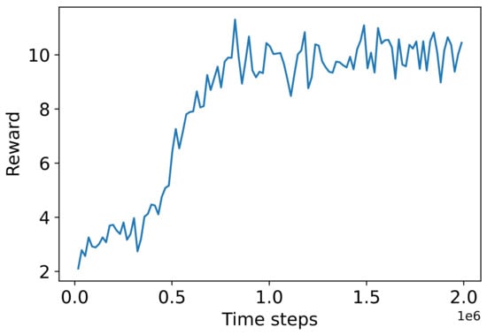
Figure 2.
Training progress using the agent parameters determined during hyper-parameter tuning.
The test simulations were reviewed, leading to the discovery of an undesirable trend. The agent will tend to increase the proportional gain and decrease the integral time until oscillations are introduced, which tend to grow until the MV oscillates between approximately 0 and 80% continuously. An example of this is shown in Figure 3. Note that the agent is only allowed to take its first action after s have elapsed. It is apparent that once the agent observes the poor performance that it has introduced, it is able to correct it in its next step. It appears that once the agent observed a long period of stable operation, it learned to select more aggressive controller parameters (high gain, low time constant), eventually leading to instability.
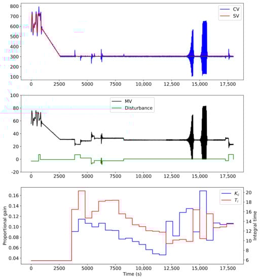
Figure 3.
Example of poor performance as a result of selecting too high a proportional gain. (Top): the controlled variable and set point variable. (Middle): the manipulated variable and input disturbance. (Bottom): the controller gains selected by the agent.
One potential explanation lies in a fault in the reward function. The reward function provides a reward of less than when the absolute value of the error exceeds . The reward will drop below when the absolute value of the error exceeds . The reward rapidly drops to approximately zero as the error increases beyond this range. As a result, the agent does not receive a signal in the form of a noticeable change in the reward when the error worsens or improves but remains greater than approximately . Therefore, the agent cannot learn the difference between small oscillations and catastrophically large oscillations. Furthermore, the agent will select controller gains that keep the error below the above-mentioned values as often as possible, even if this occasionally leads to extremely poor performance. Therefore, two adjustments will be made to the reward function, as described below in Equations (8)–(10). The first modification is to subtract the absolute value of the scaled error , while the second is to filter the SV by using a first-order filter with a two second time constant.
Subtracting the absolute value of the error relative to the range of CV values results in the minimum possible reward at any time step being approximately . The maximum reward is still . The agent receives a positive reward when and , and a negative reward for larger errors. Filtering the SV is equivalent to defining a desired response of the close loop system to SV changes. The time constant was chosen to be two times the sampling period; hence, the ideal closed-loop response will see the CV settle to within 2% of the true SV in eight seconds. An ablation study was conducted to investigate the effect of different values of and , combined with the presence or absence of SV filtering. In each case, the number of tests in which undesirable oscillations occurred, similar to those shown in Figure 3, was determined. The results are shown in Table 2. In order for a test to be counted, the oscillation had to persist for at least five minutes. Short oscillations resulting from disturbances or SV changes were not counted unless the resulting oscillation persisted for more than five minutes. Performance was assessed visually from graphs similar to Figure 3.
Table 2.
The number of tests demonstrating poor performance for each combination of reward components. The best combination of parameters has been highlighted in green.
Figure 4 shows the impact of changing the reward function. The optimal set of parameters obtained during the ablation study were used in training the agent demonstrated there. The test was identical to Figure 3, using the same starting conditions, random noise, and SV variations. Only the agent’s response differs between the two tests, owing to the change in the reward function.
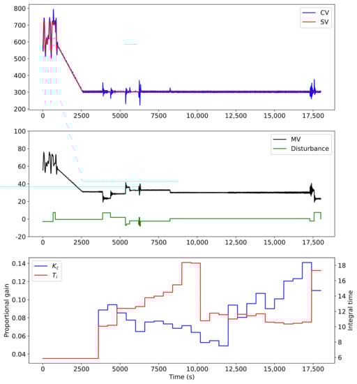
Figure 4.
Improved performance obtained using the new reward function.
Table 2 shows that, generally, filtering the SV reduces the occurrence of oscillations, unless . Increasing tends to reduce the occurrence of oscillations until the value becomes too large. As the value of is increased, the agent will prefer to avoid any overshoot or oscillation, but will also attempt to reach the SV rapidly, thus preferring an overly aggressive choice of controller gains. As a result, there is an inflection point after which increasing leads to poorer performance again. Similarly, increasing beyond can lead to a decrease in performance, possibly owing to the agent not learning that overshoot and small oscillation are still detrimental. The optimal configuration applies SV filtering and uses and , resulting in only three of the 100 tests demonstrating undesirable oscillations. This configuration also yielded the lowest overshoot on step changes in the SV. The median reward obtained in testing using this reward function and the hyper-parameters shown above was 18.76, while the average IAE was 6.90. The average IAE was 12.3 % lower than was achieved when using the original reward function. This agent was subsequently used in the industrial test.
Training was repeated using five different random number generator seeds. The minimum, maximum, and mean reward obtained during training is shown in Figure 5. The dark line represents the mean reward obtained at each step of the training, while the shaded area shows the minimum and maximum rewards at that step. The rewards obtained after approximately 750,000 training steps are sufficiently similar between training runs to conclude that the training progress does not appear to be affected by the random seed.
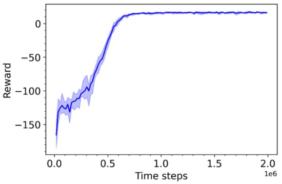
Figure 5.
Training progress over six runs with different random seeds for Agent A.
3.1.2. The Agent Using Performance Metrics Observation (Agent B)
In order to facilitate the comparison of this agent to Agent A, hyper-parameter optimization has been performed using the original reward function defined in Equations (5) and (6). This agent, with the selected hyper-parameters, was retrained using the updated reward function defined in Equation (9) and finally compared to Agent A. Hyper-parameter optimization converged on the parameters shown in Table 3 after testing a total of 368 hyper-parameter combinations. The median reward obtained by this agent was at the end of hyper-parameter tuning. An agent was trained for 2,000,000 time steps using the selected hyper-parameters. The median cumulative reward obtained during the test phase for this longer training run was , while the average IAE was . This test still used the original reward function.
Table 3.
Hyper-parameter values selected through hyper-parameter optimization.
This agent was now retrained using the reward function defined in Equation (9). The training was performed six times, each with a different random seed. The training progress is shown in Figure 6.
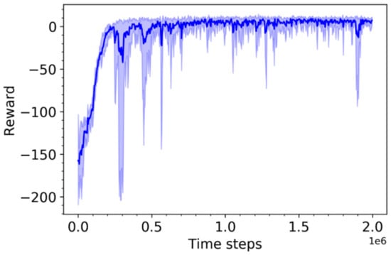
Figure 6.
Training progress over six runs with different random seeds for Agent B.
3.1.3. Internal Model Control vs. DRL Agents
The analysis described in Section 2.5.1 to determine whether the test results demonstrate a statistically significant difference between random number seeds was performed on Agents A and B. Only the minimum p-values are reported here. The minimum p-value amongst the pairs of tests for Agent A was , while for Agent B, it was 0.111. Therefore, the null hypothesis that there is no difference in performance between tests initialized with different random seeds is accepted for both agents.
Next, the performance of Agents A and B vs. IMC was ranked using Mann–Whitney tests. The results are documented in Table 4. Agent A outperforms IMC (), while Agent A also outperforms Agent B. Agent B does appear to perform slightly better than IMC, although this improvement is not statistically significant. Histograms of the cumulative rewards achieved in the test episodes for each agent are shown in Figure 7. Tests in which the cumulative reward was less than have not been plotted, although they were included in this analysis. Agent A experienced a single test achieving less than cumulative reward, while both Agent B and IMC experienced two such results. The minimum cumulative rewards achieved by Agents A, B, and IMC were , , and respectively. The maximum cumulative rewards were , , and , respectively.
Table 4.
Mann–Whitney rank test p-values for the null hypothesis that agent “1” (rows) achieves lower or equivalent cumulative rewards than agent “2” (columns). The null hypothesis is rejected when .
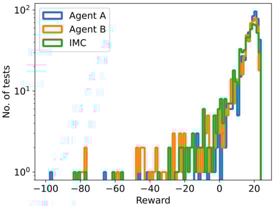
Figure 7.
Histogram of test rewards for Agents A and B, compared to IMC. Tests with rewards lower than have not been plotted.
3.2. Industrial Testing of Agent A
Performance metrics calculated from the test data are shown in Table 5 and Table 6. Measurements were recorded at one second intervals. The data set has been divided into the “Without RL” set where Agent A was not updating the controller parameters, and the “With RL” set where Agent A was in use. The number of samples in each data set, after removing time periods corresponding to interruptions to operations and operating conditions at the limits of the MV range, is indicated in the second last row of each table, followed by the time period that this represents. The distribution of the SV tracking errors, i.e., , are shown in Figure 8 and Figure 9.
Table 5.
Mill inlet water control loop performance with and without RL. The decrease percentage measures the decrease in the absolute value of the metric owing to the use of RL. Positive decreases indicate better performance, except for the reward, where an increase is expected.
Table 6.
Sump feed water control loop performance with and without the use of RL. The decrease percentage measures the decrease in the absolute value of the metric owing to the use of RL. Positive decreases indicate better performance, except for the reward, where an increase is expected.
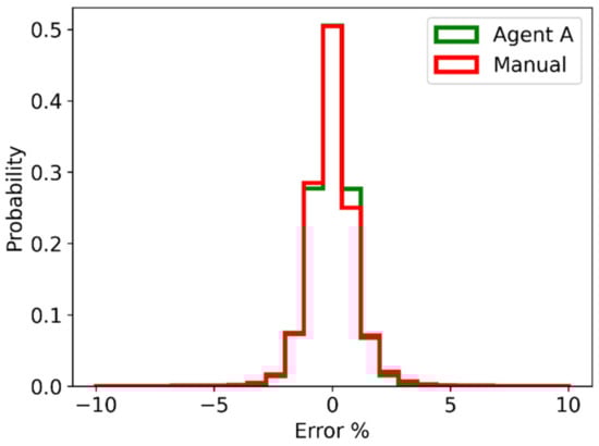
Figure 8.
Mill inlet water control loop histogram of SV tracking error as a percentage of the SV.
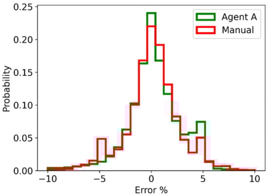
Figure 9.
Sump feed water control loop histogram of SV tracking error as a percentage of the SV.
4. Discussion
4.1. Performance in Industrial Conditions
Focusing now on the mill inlet water control loop results, as shown in Table 5, it was demonstrated that Agent A was able to outperform the manually selected controller gains. Agent A decreased the IAE and error standard deviation by 8.3 and 16.1%, respectively, although it doubled the absolute value of the mean error. Figure 8 shows that these improvements are relatively minor when considering the change in the distribution of error values.
Table 6 shows that Agent A performed substantially worse on the sump feed water control loop than the manually selected controller gains, increasing the IAE by 36% and the error standard deviation by 74%. Figure 9 shows that Agent A performed well on occasion, as it was able to increase the amount of time spent close to 0% error. Much of the performance deterioration can be attributed to the increased probability of obtaining approximately 5% error, which is linked to undesirable oscillations caused by the aggressive controller parameters selected by the agent.
The average reward obtained by Agent A on the mill inlet water loop, 0.77, can be compared to the rewards obtained during simulation testing by multiplying it by 24, the number of steps in a training episode. This yields a reward of 18.48, similar to the cumulative rewards obtained during the simulation tests, when compared to Figure 7.
4.2. Generalization to Unseen Conditions
The results presented here have shown that Agent A is able to generalize to simulation test conditions that are unlikely to have been seen in the training, owing to the use of different random seeds, as long as they do not introduce new dynamics. The training progress of Agent A was also relatively stable, as evidenced by Figure 5. In contrast, the training progress of Agent B is much more erratic and more heavily influenced by the random seed. Agent A was shown to outperform both Agent B and IMC, while Agent B did not show a statistically significant improvement in performance over IMC. Therefore, the performance metric observation space is deemed unsuitable for further use.
During early industrial testing, prior to the time period reported here, an agent was deployed that used the ARX model parameters observation space and was trained without experiencing CV discretization. The mill inlet water control loop had a continuous CV and the agent behaved sensibly here. However, the sump feed water flow rate measurement was discretized in intervals of 0.25. This agent performed poorly, selecting controller gains that were far too aggressive, resulting in an undesirable level of oscillation in the CV. In correcting this problem, the simulation was updated, as well as the number of coefficients used in the ARX model. Specifically, the number of MV coefficients was increased from 10 to 20. The reward function was also updated, as discussed in Section 3.1.1. Despite these changes, the agent continued to perform poorly, continuing to select controller gains that were too aggressive. An exponential filter was applied to the CV to produce a continuous signal, with negligible effect. As a result, this test was abandoned.
A potential hypothesis to be investigated further is that this sump feed water control loop does not fall within the range of first-order models that were used in training. Specifically, it is suspected that the time delay is longer than the maximum delay used during training.
4.3. Variation in the Agent Actions without Variation in the Underlying Process Model
During both simulation and industrial testing, the agent was observed to make unnecessary changes to the controller parameters. This does require further investigation, although some hypotheses are suggested here. Reviewing Figure 4 and Figure 10 shows that these changes often do not generate a noticeable change in behavior during training or the industrial test. One potential hypothesis is that the agent has not learned any difference between these actions and thus amplifies small differences in the observation (ARX model parameters), owing to noisy measurements, to larger differences in the controller parameters. The stability of the estimated ARX model parameters has not been tested and may also cause the observed behavior. As soon as the agent observes oscillations, it lowers the gain and increases the integral time, rectifying the problem, as seen in Figure 4 and Figure 10. This period of oscillatory behavior may provide the variety of data required to fit a usable ARX model.
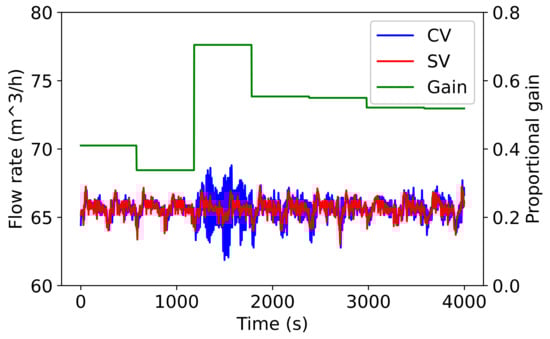
Figure 10.
An example of Agent A’s behavior during industrial testing, showing the proportional gain, CV, and SV.
4.4. Correctly Handling Shutdowns and Interruptions
During a shutdown or temporary interruption to one of the control loops used in this work, the agent does not know if it can trust the measurements, as the interruption may be related to maintenance on the actuator or measurement instrument. Furthermore, fitting the ARX model to data in which both the CV and MV are constant is not possible. If the agent should happen to select aggressive gains shortly before being interrupted, it will have to wait one hour to rectify this problem, as this is the time required to collect a new observation, after the interruption has passed. These controller parameters are acceptable under normal operating conditions but induce oscillations in response to step changes in the SV. The solution employed here is to revert to a predetermined set of conservative controller parameters that are acceptable for start-up conditions while the first observation is being acquired.
The DRL agents trained in this work are not capable of responding rapidly to such events. It is worth emphasizing that the aim of this work was to train an agent to tune PI controllers, not to replace the controllers with a DRL agent. One potential solution is to update the controller gains over much shorter timescales, e.g., less than 10 s, and to use a much shorter window of historical data, although this strays from controller tuning to non-linear control, and hence does not fit the objectives of this study. Another potential, but non-trivial, solution may be to penalize excessive overshoot and oscillations, terminating an episode with a large negative reward when such poor performance is detected. This may steer the agent towards the selection of conservative controller parameters.
4.5. Comparison of the Different Agents
The simulation test results clearly show that Agent A, using the ARX model parameters as the observation upon which actions are based, outperforms Agent B and the IMC tuning formulae, which has perfect knowledge of the plant model. At the end of the hyper-parameter optimization steps for Agents A and B, Agent A achieved a median cumulative reward of 8.97 while Agent B achieved only 8.46. Extending the training to the full 2,000,000 time steps shows that Agent B achieves a substantially lower median reward during the testing phase. Furthermore, the training progress of Agent B is erratic, as shown in Figure 6, which may explain the drop in performance resulting from longer training.
Agent A’s observation space and ARX model parameters clearly relate to how the controller gains affect reward. Variability in the reward is as a result of noise in the CV and changes in the SV. In contrast, the performance metrics observed by Agent B do not relate as clearly to the reward. The SV tracking error statistics that make up the first four values in the observation have little relation to future rewards or to the relationship between controller parameters and reward. The FFT of the error signal is related to the transfer function of the system and hence the expected reward obtained for any action, although additional information in the form of the FFT of the MV is also required. Agent B’s observation space has clear shortcomings that may explain its poor performance compared to Agent A.
4.6. Further Work
An unfortunate shortcoming of any optimization effort is that each control loop may have a slightly different reward function. For example, aiming to minimize the deviation from the SV, as done in this work, does not take into account the wear-and-tear caused by rapid actuator movements. The control loops selected in this work did not have such constraints. The ideal solution may be to derive an economic model describing the impact of deviations from the SV, as well as the cost of wear-and-tear. Unfortunately, this is challenging and poses a high barrier to entry. An alternative solution may consider exposing a higher-level error vs. actuator movement tuning interface to users, followed by retraining the agent whenever the relative importance of the two penalty terms is adjusted.
This work has treated the environment as a Markov decision process (MDP) through the assumption that the observation spaces described in Section 2.2 provide a sufficient representation of the underlying context that affects the probability distribution of the reward obtained for each action. The observation space constructed from ARX model parameters, used by Agent A, will only satisfy this requirement if there is sufficient variability in the observed data. Future work should consider treating the problem of training a general agent for multiple plants as a partially observable MDP. Recurrent neural networks [42] and meta-learning [43] may produce an agent that learns to be more robust in dealing with this challenge. Ignoring time periods with low variability in the measurements may be sufficient if the controller gains are close to optimal, although this scenario is unlikely when an agent is first deployed at a plant.
5. Conclusions
This work has demonstrated a method of applying deep reinforcement learning to the task of tuning proportional-integral control systems. A detailed simulation that included domain randomization was used to train and test the agents. Two methods of processing the time series data generated in these simulations to form an observation that the agent could use were tested: fitting an auto-regressive with exogenous inputs model to the data (Agent A) and calculating performance metrics including frequency response data (Agent B). Agent A was shown to outperform Agent B in a statistically significant number of simulated tests, and demonstrated a substantially higher median reward compared to Agent B.
Agent A was deployed at a minerals processing plant to tune the controllers on two flow rate loops: a mill inlet water flow rate and a mill discharge sump feed water flow rate. Industrial testing provided mixed results, demonstrating a marginal improvement on the mill inlet water loop and a substantial decrease in controller performance on the sump feed water loop. Several issues have been highlighted in the discussion, including unexpected behavior by the agent, where it will arbitrarily change the controller gains, challenges in generalizing beyond the transfer functions used in training the agent, and finally, implementation challenges. In spite of these shortcomings, deep reinforcement learning does show promise in automatically and continuously tuning control loops.
Funding
This research received no external funding.
Institutional Review Board Statement
Not applicable.
Informed Consent Statement
Not applicable.
Data Availability Statement
The data presented in Section 3.1 are openly available in Open Science Framework at doi:10.17605/OSF.IO/QUD9X. The data presented in Section 3.2 and Figure 10 were obtained from a third party and are not available.
Conflicts of Interest
The authors declare no conflict of interest.
Appendix A
The range within which the SV is allowed to vary must be constrained to ensure that it is physically possible to achieve the SV. The agent cannot learn successfully from a simulation in which it is impossible to achieve good performance, as every choice it makes is approximately equally bad. The training process can tolerate a small number of simulations in which the SV is not achievable, although too many will derail training, resulting in, for example, the agent learning to pick the same controller gains for all plants. The SV limits are calculated as follows:
First, the minimum and maximum possible CV values are calculated, based on the system gain, , CV offset, and MV offset, and and MV range .
The first candidate limits are selected to be 20% above and below the minimum and maximum achievable state values:
The second candidate SV limits are selected to be the CV values obtained at 30% above the minimum MV and 30% below the maximum MV:
Finally, the SV limits are the most restrictive combination of the minimums and maximums calculated here:
The clip function constrains the first argument such that, if it is smaller than the second argument, the second argument is returned. If the first argument is larger than the third argument, the third argument is returned. Otherwise, the first argument is returned.
Finally, in rare cases, it may happen that . If this occurs, the minimum is modified as follows: .
The function used to generate the SV is selected randomly with equal probability from the following functions:
- Step changes
- Ramps
- Multi-sines
- Multi-sines followed by a single ramp
In all cases, a base value is chosen in the range . This is added to the values generated by the above functions to shift the mean value of the SV.
The step-change SV generator assigns a probability of 0.1% that there will be a step change at any one step in the simulation. Where a step change does occur, the amplitude is selected from a uniform random variable in the range and multiplied by .
The ramp SV generator, similar to the step-change generator, has a probability of 0.1% that it will change the gradient of the ramp SV on each time step. Where a change occurs, the gradient is selected from a uniform random variable in the range and multiplied by . The initial ramp will always start at the base SV value selected above.
The multi-sines SV generator selects the number of sine wave components from a uniform distribution in the range . The frequency of each component is selected from a uniform distribution in the range radians. This corresponds to a maximum frequency of approximately 0.008 Hz, or a period of at least 120 s or two minutes. The phase shift of each sine wave is selected uniformly in the range . Finally, the amplitude of each sine wave is drawn from a uniform random distribution in the range . The resulting SV is obtained by summing all these sine waves.
The final SV generator starts in the same manner as the multi-sines SV generator. However, a step in the episode is chosen at random to transition from the multi-sines generator to a ramp SV. The gradient of this ramp is drawn from a normal distribution with zero mean and standard deviation of .
Note that all the SV generators clip their output to the range .
Appendix B
Table A1 lists the PPO parameters that were adjusted during hyper-parameter optimization, while Table A2 describes the range of parameters that were optimized for the multi-layer perceptron networks used in the actor and critic. Note that the optimization also included training separate actor and critic networks vs. sharing the hidden layers between the actor and critic. The parameters considered here only cover the hidden layers, as the input and output layer sizes are fixed. Note also that the output layer of the critic network will always use the linear activation function, while the output layer of the actor network will always use the hyperbolic tangent function. The tables describe the search space using a range of values; either a continuous range, e.g., , or a discrete set of values, e.g., . The distribution column shows the probability distribution from which values of each parameter are sampled. The IntUniform distribution generates integer values in the specified range with an equal probability assigned to each value. The Uniform distribution is the real-valued equivalent of this. The Log distribution uses the natural logarithm. Where the range of values is specified by a set, each value has equal probability of being selected.
Table A1.
All PPO algorithm hyper-parameters optimized in this work.
Table A1.
All PPO algorithm hyper-parameters optimized in this work.
| Parameter | Range of Values | Distribution |
|---|---|---|
| Number of workers | - | |
| Rollout length | IntUniform | |
| Value function coefficient | Uniform | |
| Entropy coefficient | Uniform | |
| Maximum gradient norm | Log | |
| Initial learning rate | Log | |
| Final learning rate | Log | |
| Discount factor () | Log | |
| GAE decay factor () | Log | |
| Number of mini-batches | - | |
| Number of optimization epochs | IntUniform | |
| Clip range | Log |
Table A2.
All MLP hyper-parameters optimized in this work.
Table A2.
All MLP hyper-parameters optimized in this work.
| Parameter | Range of Values | Distribution |
|---|---|---|
| Number of hidden layers in the policy function | IntUniform | |
| Number of hidden layers in the value function | IntUniform | |
| Number of neurons in a hidden layer | IntUniform | |
| Hidden layer activation function | - |
Note that the number of neurons in each hidden layer of the policy function and value function is treated as a separate degree of freedom in the hyper-parameter search. Therefore, each network can have between one and four layers, with each layer having a different number of neurons. Finally, the policy and value networks can share their hidden layers. The three activation functions are the hyperbolic tangent (tanh), rectified linear unit (relu), and leaky rectified linear unit (leakyrelu).
References
- Lillicrap, T.P.; Hunt, J.J.; Pritzel, A.; Heess, N.; Erez, T.; Tassa, Y.; Silver, D.; Wierstra, D. Continuous control with deep reinforcement learning. In Proceedings of the 4th International Conference on Learning Representations, San Juan, Puerto Rico, 2–4 May 2016. [Google Scholar]
- Gudimella, A.; Story, R.; Shaker, M.; Kong, R.; Brown, M.; Shnayder, V.; Campos, M. Deep Reinforcement Learning for Dexterous Manipulation with Concept Networks. arXiv 2017, arXiv:1709.06977. [Google Scholar]
- Schulman, J.; Wolski, F.; Dhariwal, P.; Radford, A.; Klimov, O. Proximal Policy Optimization Algorithms. arXiv 2017, arXiv:1707.06347. [Google Scholar]
- Cully, A.; Clune, J.; Tarapore, D.; Mouret, J.-B. Robots That Can Adapt like Animals. Nature 2015, 521, 503–507. [Google Scholar] [CrossRef] [PubMed] [Green Version]
- Silver, D.; Huang, A.; Maddison, C.J.; Guez, A.; Sifre, L.; van den Driessche, G.; Schrittwieser, J.; Antonoglou, I.; Panneershelvam, V.; Lanctot, M.; et al. Mastering the Game of Go with Deep Neural Networks and Tree Search. Nature 2016, 529, 484–489. [Google Scholar] [CrossRef] [PubMed]
- Mnih, V.; Kavukcuoglu, K.; Silver, D.; Rusu, A.A.; Veness, J.; Bellemare, M.G.; Graves, A.; Riedmiller, M.; Fidjeland, A.K.; Ostrovski, G.; et al. Human-Level Control through Deep Reinforcement Learning. Nature 2015, 518, 529–533. [Google Scholar] [CrossRef]
- Sutton, R.S.; Barto, A.G. Reinforcement learning: An introduction. In Adaptive Computation and Machine Learning Series, 2nd ed.; The MIT Press: Cambridge, MA, USA, 2018; ISBN 978-0-262-03924-6. [Google Scholar]
- Bauer, M.; Auret, L.; Le Roux, D.; Aharonson, V. An Industrial PID Data Repository for Control Loop Performance Monitoring (CPM). IFAC PapersOnLine 2018, 51, 823–828. [Google Scholar] [CrossRef]
- Visioli, A. Tuning of PID Controllers with Fuzzy Logic. IEE Proc. Control Theory Appl. 2001, 148, 1–8. [Google Scholar] [CrossRef]
- Ho, W.K.; Gan, O.P.; Tay, E.B.; Ang, E.L. Performance and Gain and Phase Margins of Well-Known PID Tuning Formulas. IEEE Trans. Control Syst. Technol. 1996, 4, 473–477. [Google Scholar] [CrossRef]
- Ho, W.K.; Hang, C.C.; Zhou, J.H. Performance and Gain and Phase Margins of Well-Known PI Tuning Formulas. IEEE Trans. Control Syst. Technol. 1995, 3, 245–248. [Google Scholar] [CrossRef]
- Chen, D.; Seborg, D.E. PI/PID Controller Design Based on Direct Synthesis and Disturbance Rejection. Ind. Eng. Chem. Res. 2002, 41, 4807–4822. [Google Scholar] [CrossRef]
- Ang, K.H.; Chong, G.; Li, Y. PID Control System Analysis, Design, and Technology. IEEE Trans. Control Syst. Technol. 2005, 13, 559–576. [Google Scholar] [CrossRef] [Green Version]
- Lu, H.; Wang, S.-Y.; Li, S.-N. Study and simulation of permanent magnet synchronous motors based on neuron self-adaptive PID. In Proceedings of the 2017 Chinese Automation Congress (CAC), Jinan, China, 20–22 October 2017; IEEE: Piscataway, NJ, USA, 2017; pp. 2668–2672. [Google Scholar]
- Xiu, J.; Wang, S.; Xiu, Y. Fuzzy Adaptive Single Neuron NN Control of Brushless DC Motor. Neural Comput. Appl. 2013, 22, 607–613. [Google Scholar] [CrossRef]
- Doerr, A.; Nguyen-Tuong, D.; Marco, A.; Schaal, S.; Trimpe, S. Model-Based Policy Search for Automatic Tuning of Multivariate PID Controllers. arXiv 2017, arXiv:1703.02899. [Google Scholar]
- Akbarimajd, A. Reinforcement Learning Adaptive PID Controller for an Under-Actuated Robot Arm. Int. J. Integr. Eng. 2015, 7, 20–27. [Google Scholar]
- Wang, X.; Cheng, Y.; Sun, W. A Proposal of Adaptive PID Controller Based on Reinforcement Learning. J. China Univ. Min. Technol. 2007, 17, 40–44. [Google Scholar] [CrossRef]
- El Hakim, A.; Hindersah, H.; Rijanto, E. Application of Reinforcement Learning on Self-Tuning PID Controller for Soccer Robot Multi-Agent System. In Proceedings of the 2013 Joint International Conference on Rural Information & Communication Technology and Electric-Vehicle Technology (rICT & ICeV-T), Bandung, Indonesia, 26–28 November 2013; IEEE: Piscataway, NJ, USA, 2013; pp. 1–6. [Google Scholar]
- Badgwell, T.A.; Liu, K.-H.; Subrahmanya, N.A.; Lie, W.D.; Kovalski, M.H. Adaptive PID Controller Tuning via Deep Reinforcement Learning. U.S. Patent 10,915,073, 25 February 2021. [Google Scholar]
- Shipman, W.J.; Coetzee, L.C. Reinforcement Learning and Deep Neural Networks for PI Controller Tuning. IFAC PapersOnLine 2019, 52, 111–116. [Google Scholar] [CrossRef]
- Deisenroth, M.P. Efficient Reinforcement Learning Using Gaussian Processes. Ph.D. Thesis, Karlsruhe Institute of Technology, Karlsruhe, Germany, July 2012. [Google Scholar]
- Pedregosa, F.; Varoquaux, G.; Gramfort, A.; Michel, V.; Thirion, B.; Grisel, O.; Blondel, M.; Prettenhofer, P.; Weiss, R.; Dubourg, V.; et al. Scikit-Learn: Machine Learning in Python. J. Mach. Learn. Res. 2011, 12, 2825–2830. [Google Scholar]
- Dhariwal, P.; Hesse, C.; Klimov, O.; Nichol, A.; Plappert, M.; Radford, A.; Schulman, J.; Sidor, S.; Wu, Y.; Zhokhov, P. OpenAI Baselines; OpenAI, 2017. Available online: https://github.com/openai/baselines (accessed on 27 February 2019).
- Andrychowicz, M.; Baker, B.; Chociej, M.; Jozefowicz, R.; McGrew, B.; Pachocki, J.; Petron, A.; Plappert, M.; Powell, G.; Ray, A.; et al. Learning Dexterous In-Hand Manipulation. arXiv 2018, arXiv:1808.00177. [Google Scholar] [CrossRef] [Green Version]
- Heess, N.; TB, D.; Sriram, S.; Lemmon, J.; Merel, J.; Wayne, G.; Tassa, Y.; Erez, T.; Wang, Z.; Eslami, S.M.A.; et al. Emergence of Locomotion Behaviours in Rich Environments. arXiv 2017, arXiv:1707.02286. [Google Scholar]
- Hallén, M. Comminution Control Using Reinforcement Learning: Comparing Control Strategies for Size Reduction in Mineral Processing. Master’s Thesis, Umeå University, Umeå, Sweden, 2018. [Google Scholar]
- Song, Y.; Steinweg, M.; Kaufmann, E.; Scaramuzza, D. Autonomous Drone Racing with Deep Reinforcement Learning. arXiv 2021, arXiv:2103.08624. [Google Scholar]
- Snoek, J. Bayesian Optimization and Semiparametric Models with Applications to Assistive Technology. Ph.D. Thesis, University of Toronto, Toronto, ON, Canada, 2013. [Google Scholar]
- Snoek, J.; Swersky, K.; Zemel, R.; Adams, R.P. Input warping for bayesian optimization of non-stationary functions. In Proceedings of the 31st International Conference on Machine Learning, Beijing, China, 21–26 June 2014; Volume 32, pp. 1674–1682. [Google Scholar]
- Gelbart, M.A.; Snoek, J.; Adams, R.P. Bayesian optimization with unknown constraints. In Proceedings of the Thirtieth Conference on Uncertainty in Artificial Intelligence, Quebec City, QC, Canada, 23–27 July 2014; p. 10. [Google Scholar]
- Lévesque, J.-C.; Durand, A.; Gagne, C.; Sabourin, R. Bayesian optimization for conditional hyperparameter spaces. In Proceedings of the International Joint Conference on Neural Networks (IJCNN), Anchorage, AK, USA, 14–19 May 2017; p. 9. [Google Scholar]
- Bergstra, J.S.; Bardenet, R.; Bengio, Y.; Kégl, B. Algorithms for hyper-parameter optimization. In Proceedings of the Advances in Neural Information Processing Systems, Granada, Spain, 12–15 December 2011; Curran Associates, Inc.: Red Hook, NY, USA, 2011; Volume 24, p. 9. [Google Scholar]
- Chapelle, O.; Li, L. An empirical evaluation of thompson sampling. In Proceedings of the Advances in Neural Information Processing Systems, Granada, Spain, 12–15 December; Shawe-Taylor, J., Zemel, R., Bartlett, P., Pereira, F., Weinberger, K.Q., Eds.; Curran Associates, Inc.: Red Hook, NY, USA, 2011; Volume 24. [Google Scholar]
- Arnold, D.V.; Hansen, N. Active covariance matrix adaptation for the (1+1)-CMA-ES. In Proceedings of the 12th Annual Conference on Genetic and Evolutionary Computation—GECCO ’10, New York, NY, USA, 7–11 July 2010; ACM Press: Portland, OR, USA, 2010; p. 385. [Google Scholar]
- Hansen, N. A CMA-ES for Mixed-Integer Nonlinear Optimization; INRIA: Rocquencourt, France, 2011; p. 13. [Google Scholar]
- Igel, C.; Hansen, N.; Roth, S. Covariance Matrix Adaptation for Multi-Objective Optimization. Evol. Comput. 2007, 15, 1–28. [Google Scholar] [CrossRef] [PubMed]
- AIworx AIworx-Labs/Chocolate. Available online: https://github.com/AIworx-Labs/chocolate (accessed on 13 February 2021).
- The Linux Foundation® ONNX|Home. Available online: https://onnx.ai/ (accessed on 3 March 2021).
- Microsoft ONNX Runtime|Home. Available online: https://www.onnxruntime.ai/ (accessed on 3 March 2021).
- Brown, R.G. Exponential Smoothing for Predicting Demand 1956. Available online: https://www.industrydocuments.ucsf.edu/tobacco/docs/#id=jzlc0130 (accessed on 23 February 2021).
- Hausknecht, M.; Stone, P. Deep Recurrent Q-Learning for Partially Observable MDPs. arXiv 2015, arXiv:1507.06527. [Google Scholar]
- Finn, C.; Abbeel, P.; Levine, S. Model-Agnostic Meta-Learning for Fast Adaptation of Deep Networks. arXiv 2017, arXiv:1703.03400. [Google Scholar]
Publisher’s Note: MDPI stays neutral with regard to jurisdictional claims in published maps and institutional affiliations. |
© 2021 by the author. Licensee MDPI, Basel, Switzerland. This article is an open access article distributed under the terms and conditions of the Creative Commons Attribution (CC BY) license (https://creativecommons.org/licenses/by/4.0/).