Article

Magnetic Preconcentration and Process Mineralogical Study of the Kiviniemi Sc-Enriched Ferrodiorite

1
Oulu Mining School, Faculty of Technology, University of Oulu, P.O. Box 3000, FI-90014 Oulu, Finland
2
Process Metallurgy, Faculty of Technology, University of Oulu, P.O. Box 3000, FI-90014 Oulu, Finland
*
Author to whom correspondence should be addressed.
Minerals 2021, 11(9), 966; https://doi.org/10.3390/min11090966
Submission received: 20 July 2021 / Revised: 28 August 2021 / Accepted: 1 September 2021 / Published: 4 September 2021
(This article belongs to the Section Mineral Processing and Extractive Metallurgy)

Abstract

:
Scandium is classified as a critical raw material by the European Union. Its beneficiation from various primary and secondary sources is currently being studied under several research and development projects. Due to the geochemical characteristics of Sc, its enrichment to ore grades by geological processes is scarce. Potential new sources are investigated to respond to the expected increasing demand for this rare earth metal. The recently discovered Kiviniemi Sc deposit in Finland represents an igneous occurrence with estimated total resources of 13.4 Mt and an average Sc grade of 163 g/t. The deposit consists of relatively homogeneous ferrodioritic intrusive body with its main unit with ~2.5 ha surface extension. Scandium is mainly incorporated into the lattice of clinopyroxene and amphibole within the main unit. Composite samples from three drill cores from various parts of the main unit were concentrated with a combination of low-intensity and high-gradient magnetic separation. Depending on the feed characteristics, high-gradient magnetic separation reached recoveries between 87% and 92% with 230–310 ppm Sc while removing 35–49 mass percent of gangue minerals, mainly plagioclase and potassium feldspar. Our study provides information on the magnetic preconcentration conditions with process mineralogical details and produced concentrates for further testing according to the suggested processing scheme.

1. Introduction

The fifteen lanthanides plus scandium and yttrium are classified as rare earth elements [1]. Due to its small ionic radius, Sc behaves differently from the rest of the group (Sc 75 pm in octahedral coordination, while lanthanides range from 103 to 86 pm [2]). This attribute makes Sc a moderately compatible element fitting into the lattice of common ferromagnesian rock-forming minerals, particularly pyroxene, amphibole and garnet, despite being a trivalent cation [3]. The similarity of the ionic radius of Sc3+ with those of Mg2+ and Fe2+ (78 and 72 pm, respectively) allows Sc to substitute for Mg or Fe in the M1 octahedral site in clinopyroxene and is also suggested to enter the M3 sites in the amphibole structure [4,5]. The average Sc abundance in the bulk continental crust is 22 ppm [6]. Mafic rocks contain on average 30–40 ppm scandium, whereas in felsic rocks, the abundance is less than 20 ppm [7].
Geological formations in which Sc is enriched can be divided broadly into primary deposits related to igneous and hydrothermal processes and secondary deposits where Sc has been concentrated by sedimentary processes and weathering, producing laterite and placer deposits [8]. Considering igneous rocks, the low concentration of Sc in magmatic melts coupled with the moderately compatible nature of Sc promotes the dispersion of Sc into ferromagnesian minerals at the early stages of crystallization. Due to the geochemical characteristics of Sc, its enrichment to ore grades by geological processes is scarce. Consequently, the estimated global Sc production is only 15 t [3,9]. Table 1 summarizes the main features of selected Sc deposits, both those that are currently under production, such as Bayan Obo and those that are in various development stages. At Bayan Obo, scandium is recovered from the tailings of other REE and iron production [3]. According to Wang et al. (2020) [10], magmatic rocks with average Sc concentrations > 60 ppm can be regarded as Sc deposits. Table 1 includes the Kiviniemi ferrodiorite-hosted Sc deposit discovered recently in eastern Finland [11].
With respect to REE production from ore to end products, after the traditional beneficiation of REE minerals, individual elements are extracted by hydrometallurgy, electrometallurgy or pyrometallurgy, of which hydrometallurgy is the most widely used technique. The purified bulk product is often a solid oxide, carbonate or chloride with very low impurity content, which is then further processed into desired end-products [17,18,19]. All past and current production of Sc is from tailings of Ni, Al, Ti, REE, U and Zr ores [17]. For example, bauxite residues or so-called red mud, which is the main waste product of the Bayer process and generally contains 40–100 ppm Sc, have been studied in recent decades as a possible secondary resource of Sc [20,21,22]. Problems have arisen in hydrometallurgical processing from the non-selective mobilization of Fe and Ti, which tend to deteriorate the purification and precipitation of suitable Sc products. According to Yagmurlu et al. [23], a combination of pyrometallurgical and hydrometallurgical processes shows promising results for the sustainable recovery of Sc from red mud with selective iron recovery. Additionally, Li et al. [21,24] conducted experiments with reductive roasting pre-treatment of red mud residue, in which hematite and goethite are reduced to metallic iron, followed by magnetic separation. The selective reduction of ferrous oxide in a system containing Sc2O3 is based on the differences in the thermodynamic properties of the oxides. The high stability of Sc2O3, in comparison to ferrous and ferric oxides in particular, provides the theoretical foundation for the reduction and separation of metallic products from Sc2O3-containing materials [25,26].
The major applications of Sc include solid oxide fuel cells (SOFCs) in which scandium acts as a stabilizing agent for the solid electrolyte; Al–Sc alloys, in which Sc contributes to their strength and weldability; mercury vapor high-intensity lights; and an activator ion in TV or computer monitors. In comparison to Y, Sc has much better electrical conductivity, heat-treatment and strengthening dopant properties in addition to its known application in high-performance lighting and, therefore, this can outweigh its cost disadvantage in many applications [22].
The GTK mineral processing laboratory Mintec carried out preliminary beneficiation tests with samples from Kiviniemi mafic intrusion in 2010 [27]. Magnetic separation conducted with a combination of low-intensity and high-gradient magnetic separation (HGMS) resulted in a mineral concentrate with ~346 ppm Sc at a recovery level of ~72% and was, therefore, suggested to be the concentration method with the greatest potential for Sc-bearing minerals of the deposit. Furthermore, acquired concentrates were leached with acids. The best dissolution results were obtained with a mixture of hydrogen fluoride and hydrochloric/sulfuric acid. However, the solubility of Fe from ferrous silicates, which are the main carriers of Sc2O3, was almost thousand-fold in comparison with Sc and this type of processing would require large quantities of acids and produce large volumes of materials, which would need to be managed by further processing. The flotation experiments performed in this preliminary beneficiation study were unsuccessful [27]. To overcome the issues introduced to hydrometallurgical processing by Fe, we suggest a new processing scheme for the Kiviniemi-type deposits (Figure 1). This proposition introduces the preconcentration stage with conventional magnetic methods followed by pyrometallurgical treatment for the reduction and removal of Fe prior to hydrometallurgical processes. The main aim of the magnetic beneficiation step is to maximize the recovery of Sc2O3 while minimizing the alkali-containing diamagnetic plagioclase and potassium feldspar in the concentrate.
In this study, results of the magnetic beneficiation step of the suggested processing scheme for the selected Kiviniemi ferrodiorite composite samples are presented. Magnetic separation experiments were carried out and supplemented with a process mineralogical study. Specifically, the magnetic separation with a combination of low-intensity (LIMS) and pulsating high-gradient magnetic separation (HGMS) with SLon® and the characteristics of the resulting concentrates and tailings were investigated. The main target was to obtain information regarding possible preconcentration conditions with process mineralogical characteristics of the Kiviniemi composite samples and provide concentrates for further testing according to the suggested processing scheme (Figure 1).

2. The Kiviniemi Intrusion

The Kiviniemi mafic intrusion (Figure 2A,B) is located in the municipality of Rautalampi, approximately 70 km SW of the city of Kuopio in Finland [11,16]. Altogether, nine holes were drilled between 2008 and 2010. As illustrated in Figure 2A, the Kiviniemi intrusion has a zoned structure, in which an Fe- and Sc-rich, medium- to coarse-grained garnet-bearing fayalite ferrodiorite body is surrounded by transitional ferrodiorites and pyroxene ferromonzodiorites. The country rock of the intrusion is composed of porphyritic granite [11]. The preliminary mineral resource estimation calculated with the inverse distance method is 13.4 Mt, with an average grade of 163 g/t Sc [11,16]. In addition, 1726 g/t Zr and 81 g/t Y have been reported.
All of the ferrodiorites and leucoferrodiorites at Kiviniemi show broadly similar mineral paragenesis, with the main minerals being (ferro)hedenbergitic clinopyroxene, almandine garnet, fayalitic olivine (Fo1–4), amphibole (ferropargasite and ferroedenite) and plagioclase (average An ca. mol-40%) [11]. According to Halkoaho et al. (2020) [11], the main carriers of Sc at Kiviniemi are amphiboles ferropargasite and ferroedenite (with max. Sc2O3 2088 ppm), clinopyroxene (ferro)hedenbergite (max. Sc2O3 1736 ppm) and fluorapatite (max. Sc2O3 1133 ppm). The grain sizes of the main minerals range typically between 100 and 2000 µm [27]. Accessory minerals include ilmenite, fluorapatite, zircon, magnetite, biotite, pyrite, pyrrhotite, quartz and microcline. Ilmenite is the most common accessory mineral occurring as inclusions, exsolution lamellae and skeletal aggregates with magnetite, hematite, pyrite and pyrrhotite [11].

3. Materials and Methods

After the drilling program at Kiviniemi, GTK sampled the cores, which were analyzed systematically at Eurofins Labtium Oy [16]. For this study, three adjacent or proximal drill core samples (Figure 3) were included from a total of four drill core intervals (total of 12 samples). These were processed into four composite samples to provide sufficient material for laboratory-scale experiments. The samples are coded and referred to accordingly: R1 composite sample from drill core R1; R2/upper (R2/u) and R2/lower (R2/l) composite samples from drill core R2; and R3 composite sample from drill core R3 (Figure 2 and Figure 3). In these samples, medium- to coarse-grained garnet-bearing fayalite ferrodiorite is the prominent rock type which contains most of the Sc at Kiviniemi [11,28]. The selection of the samples was based on the availability of suitable samples provided by GTK, the dimensions of the deposit and the average Sc grade estimated for the deposit.
Samples were delivered to Oulu Mining School as crushed drill core material (<4 mm) from GTK. Samples were then split with a sample splitter, half of which were processed for magnetic separation experiments. Split samples were first dry sieved with a Retsch sieve shaker (10 min with amplitude 1.5 mm). The coarser fractions (>125 µm) were combined and ground with a Wedag rod mill (H × D = 30.5 cm × 15 cm) with a constant rotation frequency of 100 rpm. Furthermore, 11 stainless steel rods (7 pcs 30 cm × 1.9 cm and 4 pcs 30 cm × 1.4 cm) with a total mass of 7.05 kg and a solid percentage of 60% were used in wet grinding. Samples were ground as approximately 1 kg aliquots for 1 h, after which they were dried, combined and mixed thoroughly with fine fractions. A suitable subsample was then wet screened to determine the particle size distribution. The target P80 close to or less than 90 µm was considered appropriate at the beginning of the study, which is suitable for magnetic separation with SLon and would enable possible flotation experiments also considered as an option at the beginning of the study. The comminution procedure was maintained constant for all the samples included in this study.
The properties of Sc-bearing silicates, the bulk mineralogy of the deposit and the textural features provide the criteria for the selection of beneficiation procedures. Considering the physical characteristics of the Kiviniemi main Sc-bearing minerals, clinopyroxene and amphibole, with an average density of 3.5 g/cm3 and the dominant gangue minerals, plagioclase and potassium feldspar with an average density of 2.6 g/cm3, the concentration criterion (CC) of 1.57 falls into the range of very difficult separation with respect to gravity concentration [29,30]. However, with respect to mass magnetic susceptibility properties, the chemical composition of the minerals is the main controlling factor, with Fe but also Mn and Cu contents having the main effects on the extraction efficiency of paramagnetic minerals [31,32,33]. Therefore, due to the main occurrence of Sc in ferrous, paramagnetic minerals [11,34,35], wet magnetic separation with a combination of low-intensity magnetic separation (LIMS) and SLon pulsating high-gradient magnetic separator (HGMS) was chosen for the preconcentration. The SLon utilizes a combination of magnetic force, pulsating fluid and gravity to continuously separate magnetic and non-magnetic minerals [36]. The pulsation in the separation zone enhances the separation performance by agitating the slurry and keeping all particles in a dispersed state while minimizing entrapment. This mechanism also maximizes the particle accumulation on the rod matrix, creating a more usable surface area for the collection of magnetics [36,37]. SLon magnetic separators treat materials with a wide range of throughputs from 100 g per batch in SLon-100 cyclic pilot-scale magnetic separator to several hundred t/h in full-scale separators [38]. With SLon, the effect of magnetic induction (0.3–1.0 T) and the frequency of pulsation (50–250 rpm) were investigated. Wet magnetic separation tests with LIMS WD (20) 111-15 and SLon 100 were carried out at the laboratories of Metso Outotec Research Centre, Pori, Finland. Experimental parameters were selected based on information from earlier beneficiation study [27], characteristics of paramagnetic mineral separation with Slon [38] and characteristics of the feed [11,34,35]. SLon separations were conducted for ~200 g batches.
To obtain optimal analytical results in the preliminary resource estimation, different analytical methods on core samples were tested, such as X-ray fluorescence (XRF), inductively coupled plasma–optical emission spectrometry (ICP-OES) and inductively coupled plasma–mass spectrometry (ICP-MS) [28]. The most reliable results were obtained with ICP-MS and ICP-OES after fusion with sodium peroxide. In this study, ICP-OES was chosen as the quantitative bulk elemental analysis method and all analyses were conducted with an accredited method (721P) by Eurofins Labtium in Kuopio, Finland. Dry samples were pulverized to 100%—90 µm with a tungsten carbide mill at Oulu Mining School prior to sending for analysis. For ICP-OES analysis, a prepared pulp sample (0.2 g) was fused with anhydrous sodium peroxide in zirconium crucible by heating in an electric furnace at 700 °C for one hour. The melt was dissolved in hydrochloric acid. The final solution was diluted with water prior to instrumental analysis. The routine method is the analysis of 27 elements with ICP-OES Thermo Electron ICAP 6500 Duo. Detection limits with quality control details are provided as electronic Supplementary Data (Table S1).
Automated mineralogy is a well-established technique which can be applied with optimized scanning electron microscopes (SEMs) and usually several X-ray detectors, such as silicon drift detectors (SDDs) [39,40]. With stage automation and particle analysis software packages, such as Oxford Instruments INCAMineral, in combination with the post-processing software GrainAlyzer, data on modal mineralogy, liberation characteristics and associations can be produced, processed and presented. In this study, the INCAMineral software (Version 5.05) and Zeiss ULTRA Plus instrument (FESEM, Field Emission Scanning Electron Microscope) at the Centre of Material Analysis (CMA), University of Oulu, were used on polished vertical blocks of all concentrates and tailings. Graphite was added to the samples to minimize the effects of touching particles. Applied instrumental parameters of acceleration voltage 15 kV, beam current 2.3 nA and working distance 8.3 mm were used. A minimum of 10,000 detected features were set for each sample.
For mineral compositional analysis, a JEOL JXA-8530FPlus electron probe microanalyzer was used at the CMA, University of Oulu. Analyses were carried out on polished blocks on all composite samples. The analytical conditions were an accelerating voltage of 15 kV, a beam current of 15 nA and a beam diameter 10 µm. Data on detection limits and the standards used are provided as electronic Supplementary Data (Table S2).

4. Results

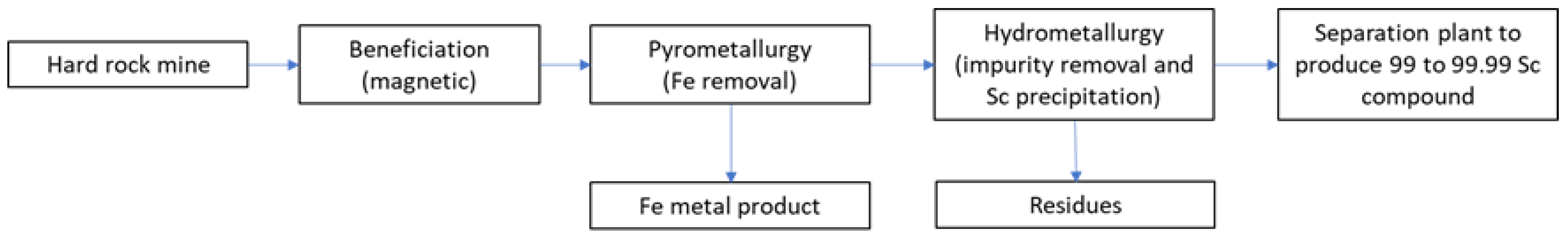
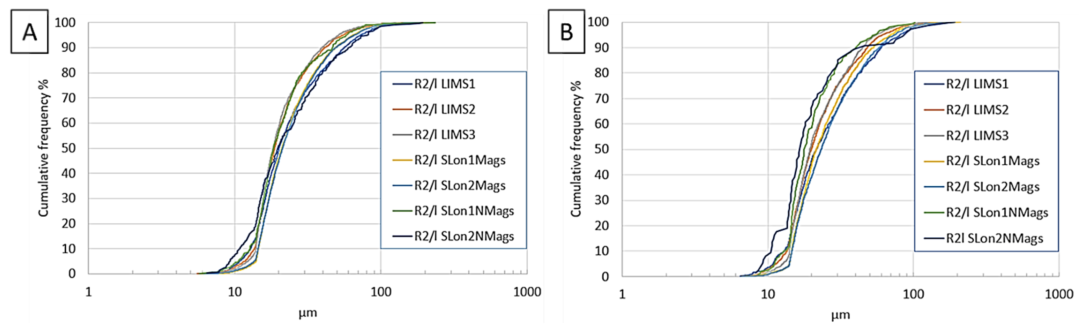
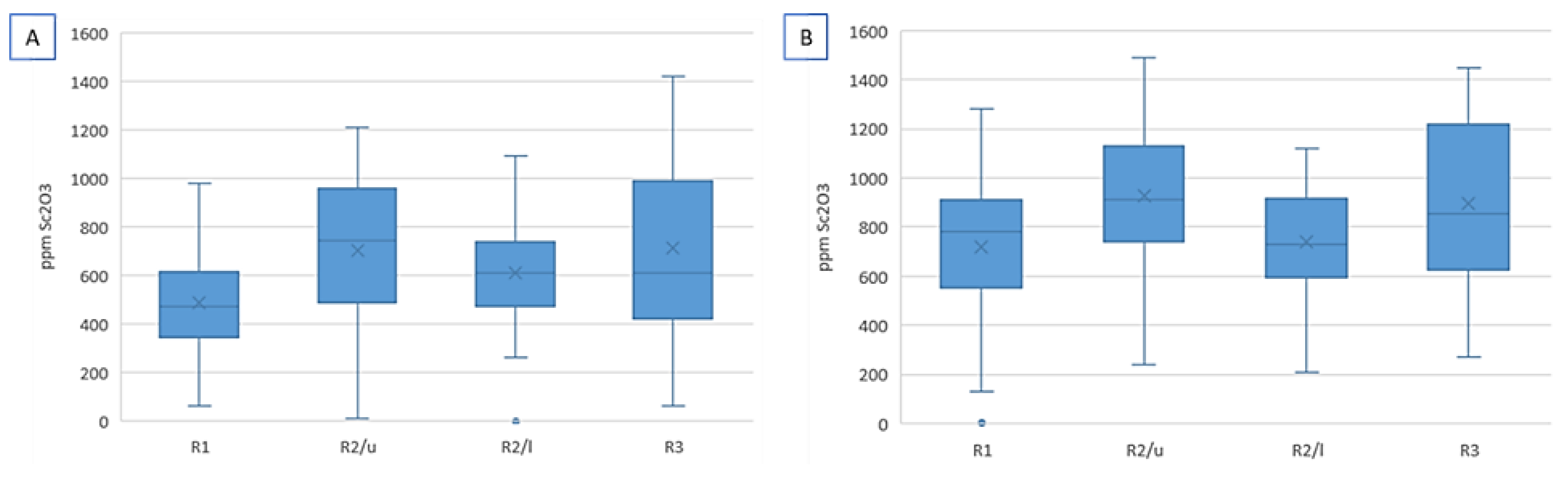
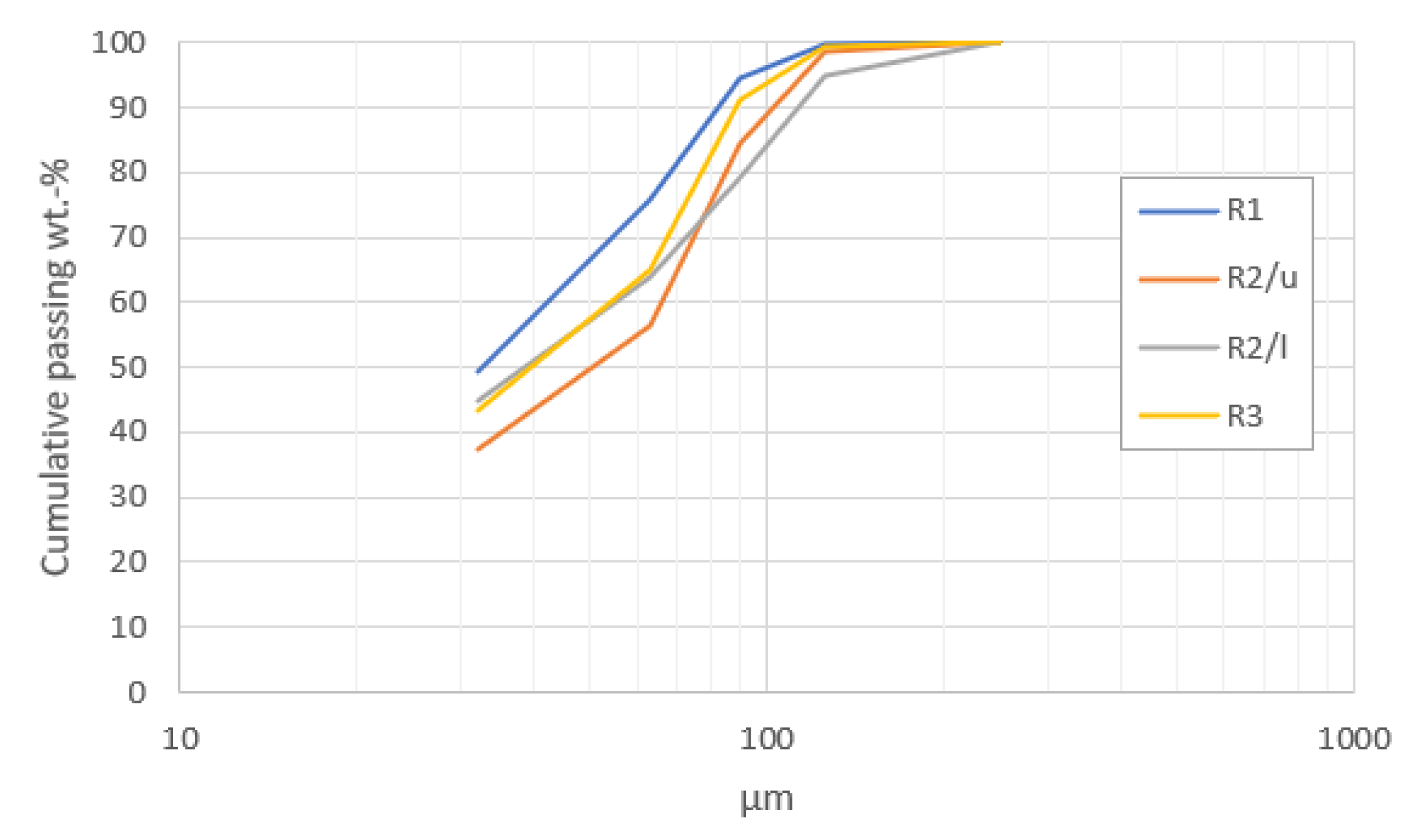
4.1. Feed Particle Size Distribution and Chemical Compositions

The particle size distributions for composite samples of each drill core after comminution are presented in Figure 4. The target P80 for samples was close to or less than 90 µm, which was achieved with wet grinding for 60 min. However, the samples from the upper parts of the intrusion contained more fines after the grinding; sample R1 from the upper parts of the intrusion contained almost 50% < 32 µm after comminution. This is attributed to the more extensive alteration compared to the samples from the lower parts, based on observations in microscopic examination. Chemical data (ICP-OES) received from GTK for each individual drill core sample are presented in Table 2.
As half of the drill core samples were processed and combined into composite samples for magnetic separation, the calculated weighted average compositions are also presented in Table 2. All the fayalite ferrodiorite samples have very low MgO contents and are enriched in FeO and P2O5. The Al2O3, K2O and SiO2 contents are highest in the R3 samples, while their FeO content appears to be lower than in the other drill core samples and lower than the ferrodiorite average (23.1 ± 3.7), as reported by Halkoaho et al. (2020) [11]. The average Sc2O3 contents of the composite samples in Table 3 correspond to 160, 202, 174 and 174 ppm Sc for R1, R2/u, R2/l and R3, respectively.

4.2. Magnetic Separation

LIMS provided three magnetic fractions (Mags1, Mags2 and Mags3) and non-magnetic fraction (NMags), which continued to SLon separations. The three magnetic LIMS fractions removed, in total, 9.5, 9.0, 9.6 and 8.0 mass% of the feed for R1, R2/u, R2/l and R3 composite samples, respectively, with most of the ferromagnetic material removed into the first fraction. Details on the LIMS magnetic fractions are provided as electronic Supplementary Data (Figure S1). Grades for combined LIMS magnetic fractions were 110, 163, 153 and 167 ppm Sc for R1, R2/u, R2/l and R3 samples with corresponding recoveries of 7.1%, 7.1%, 8.5% and 7.4% Sc, respectively. The feed grades for SLon experiments after LIMS (LIMS NMags) were 150, 210, 170 and 180 ppm Sc for R1, R2/u, R2/l and R3 samples, respectively.
The first five SLon rougher separations were performed on the R2/l composite sample, using three different pulsation frequencies (50, 150 and 250 rpm) and applied magnetic induction of 0.3, 0.5 and 1.0 T. At first, the effect of various pulsation frequency was tested with the magnetic induction of 0.5 T, after which magnetic induction 0.3 and 1.0 T were tested with selected pulsation frequency of 150 rpm. In addition to the first five rougher tests, two sets of rougher–cleaner tests were carried out for the R2/l composite sample with a 3 mm matrix, pulse frequency of 150 rpm and varying applied magnetic induction from 0.5 to 1.0 T (Rougher1a and Cleaner1b) and from 0.7 to 1.0 T (Rougher2a and Cleaner2b). A summary of the first five rougher experiment results and two rougher–cleaner experiments performed on the R2/l composite sample are presented in Table 3.
Increasing the pulse frequency at the rougher stage from 50 to 250 rpm resulted in an increasing grade (from 220 to 250 ppm Sc) but a decreasing recovery from 91% to 77% with the applied magnetic induction of 0.5 T. This implies that the higher frequency of pulsation causes the fine paramagnetic particles to be dragged out by hydrodynamic forces [38]. On the other hand, a 150 rpm pulse frequency coupled with an increase in applied magnetic induction from 0.3 to 1.0 T appears to decrease the grade slightly from 260 to 250 ppm, which is within the limits of analytical error (standard deviation from duplicate samples ± 7 ppm). However, there is an increase in recovery from 83% to 92% with a higher applied magnetic induction. Based on these results, the effect of pulse frequency is more significant to the recovery at the rougher stage than the applied magnetic induction strength. Furthermore, optimizing the rougher recovery at 150 rpm pulsation, the highest applied magnetic induction appears to provide the best results. Regarding the cleaner stages, according to these results, the grade is only slightly improved to reach the value of 270 in the first cleaner test, while the recovery is quite significantly reduced to 78%. The second cleaner test did not improve the grade, with only slight improvement to the recovery.
After the first set of SLon experiments for the R2/l composite sample, two sets of experimental parameters targeting high recoveries were also chosen to run composite samples R1, R2/u and R3. These test parameters were 1 = 50 rpm pulsation with 0.5 T and 2 = 150 rpm pulsation with 1.0 T. The purpose of this was to obtain more information on the variability and validity of the magnetic separation for the Kiviniemi-type fayalite ferrodiorite and the results are presented in Table 4. An improvement in the quality of concentrates was more obvious for the R1and R2/l composite samples with 150 rpm pulsation and 1.0 T applied magnetic induction, whereas considering the R2/u and R3 samples, the effect appeared similar although smaller in magnitude.

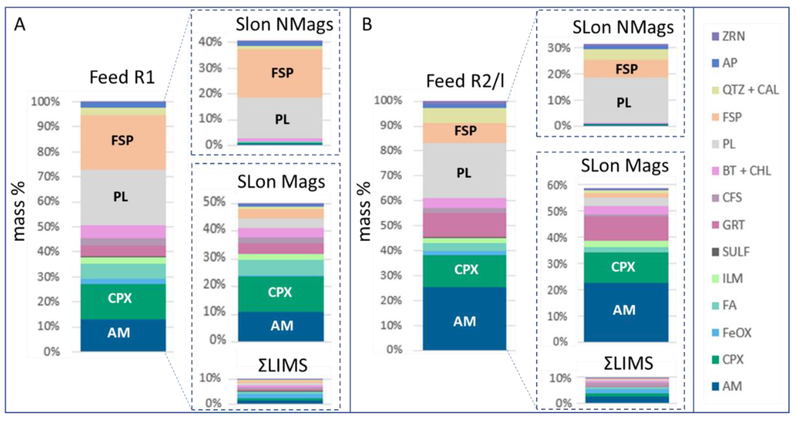
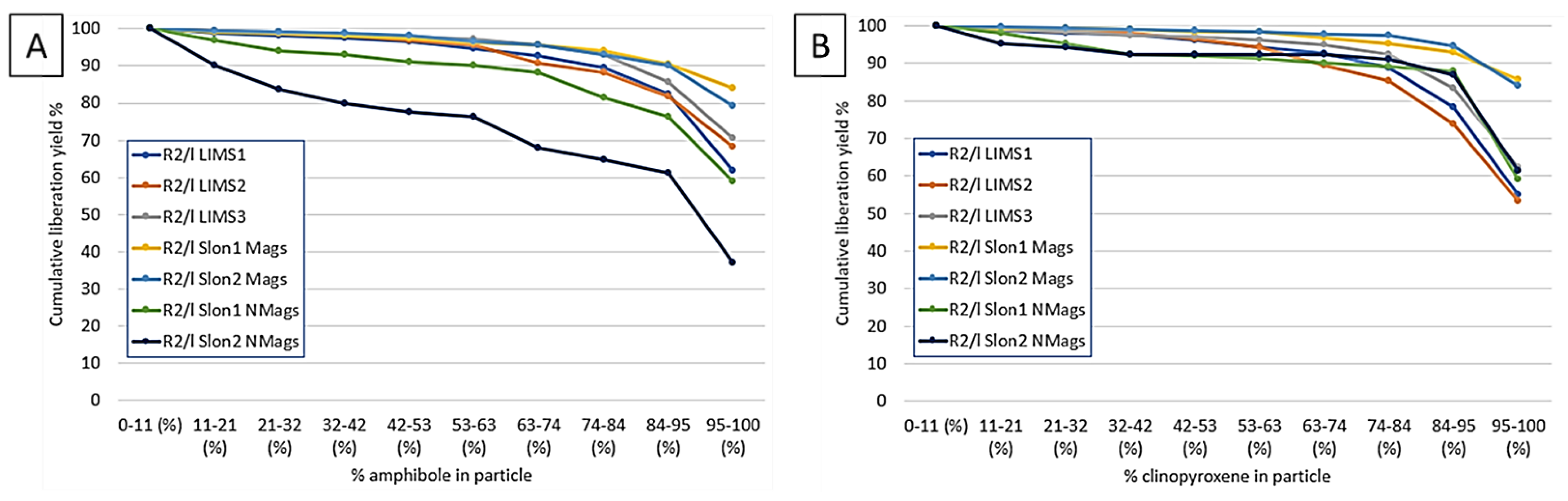
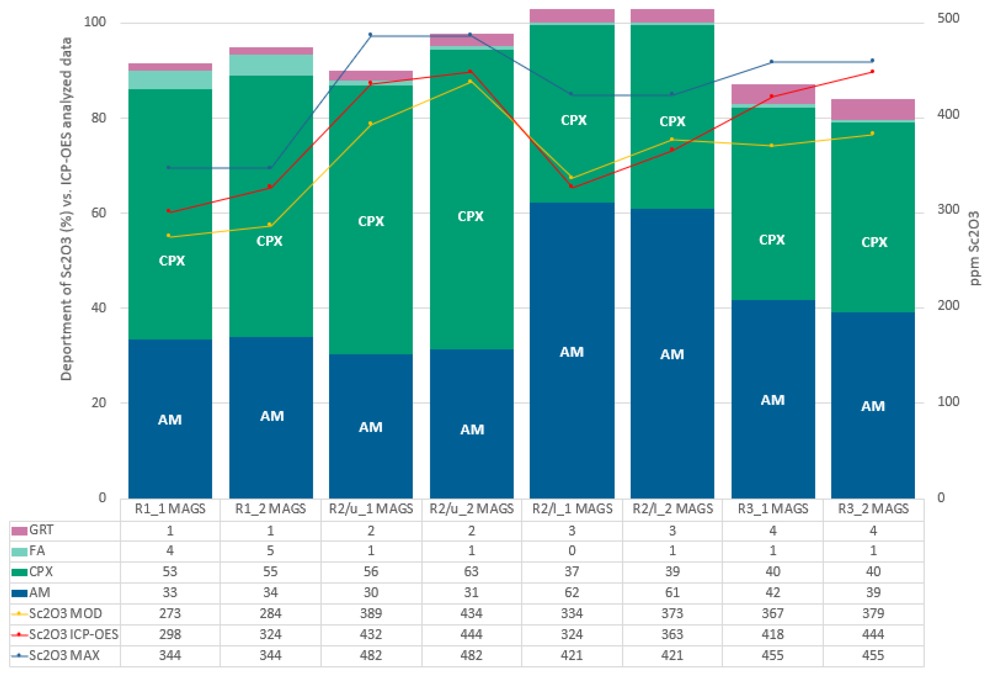
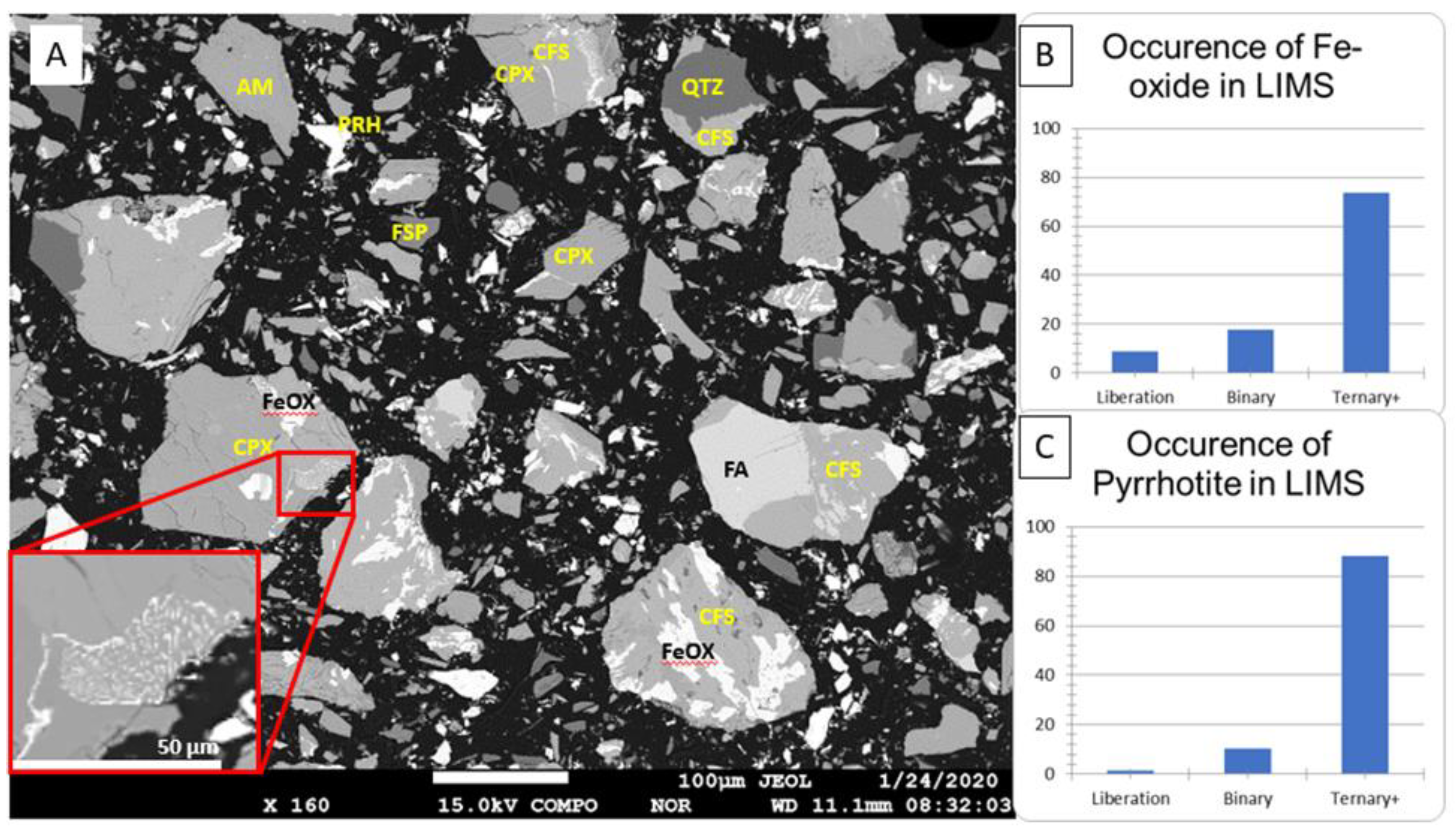
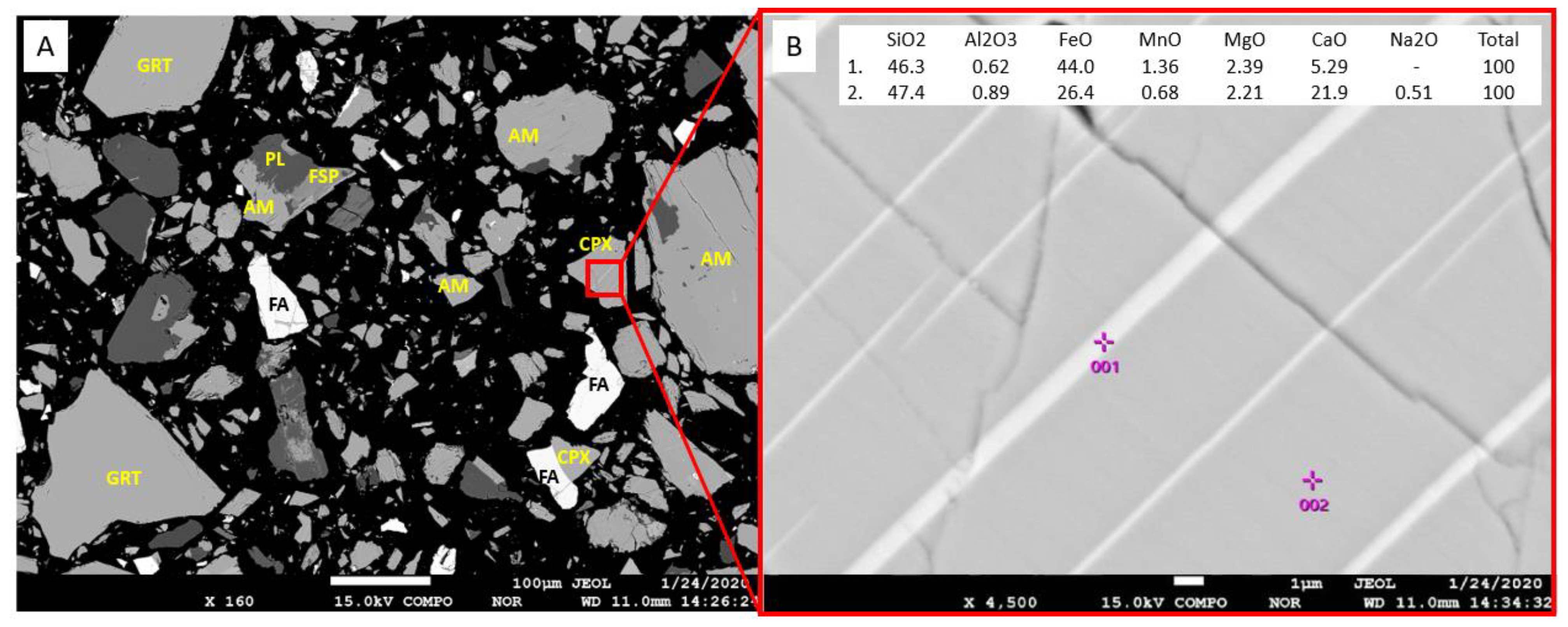
4.3. Process Mineralogical Features

An example of the amphibole and clinopyroxene grain size distribution data in terms of ECD (equivalent circle diameter) in R2/l concentrates and tailings after post-processing INCAMineral data with GrainAlyzer is presented in Figure 5A,B. Descriptive statistics on the grain sizes of amphibole and clinopyroxene in all concentrates and tailings are presented in electronic Supplementary Data (Table S3). The trend is similar particularly for clinopyroxene in all composite samples, with coarser grains separated into LIMS and SLon magnetic fractions. Depending on the frequency of the pulsation, hydrodynamic drag pulls some amount of finer paramagnetic grains and mixed particles into the tailings. However, the applied magnetic induction is sufficient for this effect to be quite minimal, which is supported by ICP-OES assays and modal mineralogy.
The modal mineralogy for calculated feed, combined LIMS magnetic fractions (ƩLIMS), SLon magnetic fraction (SLon Mags) separated with 150 rpm and 1.0 T and corresponding tailings (SLon NMags) are presented as the mass% of the total material flow for R1 and R2/l composite samples in Figure 6A,B, respectively. Data on the modal mineralogy for all samples are provided as electronic Supplementary Data (Table S4). The amount of amphibole in the R2/l feed sample is significantly higher (~25 mass%) than in the other samples (13–15 mass%), while the amount of potassium feldspar is lower (~8 mass%) than in the other composite samples (16–24 mass%).
LIMS efficiently removes particles containing ferromagnetic minerals, magnetite and monoclinic pyrrhotite, into the magnetic fractions. Total iron oxide plus pyrrhotite recovery to the LIMS fractions is usually greater than 70%. As magnetite and pyrrhotite both occur on the grain boundaries, as inclusions and particularly magnetite in complex symplectic mineral intergrowths (enlargement in Figure 7A) and reaction rims, ternary occurrences account for most of the magnetite (generally >70%, Figure 7B) and pyrrhotite (>80%, Figure 7C) occurrences. These types of textures resulted in relatively high mass % of LIMS concentrates in all the composite samples, considering that the sum for feed magnetite and sulfides varied between 1.7 and 2.6 mass%. In addition to magnetite and pyrrhotite, a significant proportion of the feed clinoferrosilite was deflected into the LIMS magnetic fraction.
A back-scattered electron image of SLon R2/l _2 concentrate is provided in Figure 8A with a detail on exsolution lamellae in clinopyroxene in Figure 8B, which was a common feature in all composite samples. According to Halkoaho et al. (2020) [11], lamellae are probably clinoferrosilite, which is also indicated in EDS analysis results (Figure 7B) in this study. With respect to magnetic separation, this type of iron-rich lamellae promotes the magnetic separation of clinopyroxene, which is supported by negligible losses to tailings.
Amphibole and clinopyroxene both occur mainly as liberated grains, particularly in the R2/u and R2/l (Figure 9A,B) SLon concentrates due to the primary coarse-grained character of the Kiviniemi ferrodiorite rocks and relatively fine grinding of the feed. In LIMS magnetic fractions and SLon tailings, occurrences of mixed particles increase. The main association for both amphibole and clinopyroxene in tailings is with plagioclase and potassium feldspar. Mineral associations of amphibole and clinopyroxene in all concentrates and tailings are provided as electronic Supplementary Data (Table S5a–d).
The average chemical compositions of amphibole and clinopyroxene from each four composite samples are presented in Table 5. The average Sc2O3 contents of amphibole vary between the lowest value of 489 ppm in the R1 composite sample to 710 ppm in the drill core R3 composite sample. The average Sc2O3 content of clinopyroxene is higher in every composite sample than the corresponding amphibole Sc2O3 content. In the composite sample from drill core R3, the average Sc2O3 contents are high for both minerals: 710 and 898 ppm for amphibole and pyroxene, respectively (Table 5 and Figure 10), with similar levels for the R2/u composite sample. Details on the variation of the Sc2O3 content (ppm) in both amphibole and pyroxene are presented as box and whisker plots in Figure 10A,B, respectively.

5. Discussion

According to Halkoaho et al. (2020) [11], the main carriers of Sc in the ferrodiorites are amphibole (103–2088 ppm Sc2O3, n = 27), clinopyroxene (818–1736 ppm, n = 29) and apatite (1062 and 1133 ppm, n = 2). Furthermore, zircon contains on average 187 ppm Sc2O3 with Sc2O3 contents also detected in garnet (44–343 ppm, n = 6), clinoferrosilite (0–199 ppm, n = 13) and plagioclase (22–175 ppm, n =18) [11]. Similar results were observed in the analyses conducted in this study. In addition to the main Sc carriers, amphibole and clinopyroxene, Sc2O3 was detected mainly in garnet (0–260 ppm, n = 39), fayalite (0–220 ppm, n = 33) and zircon (0–300, n = 15). Results above the detection limits (>100 ppm) were also occasionally observed for ilmenite, clinoferrosilite, plagioclase and potassium feldspar. A summary of EPMA results for other minerals is provided as electronic Supplementary Data (Table S6). As presented in Table 5 and Figure 10, Sc2O3 contents in both main carriers exhibit wide variation in all composite samples. Further studies with methods such as high-resolution laser ablation mass spectrometry (LA-SC-HR-ICP-MS), which is more suitable for high-accuracy trace element analysis than EPMA, might provide further insight into this phenomenon. Furthermore, this type of analysis should be preferably conducted on uncrushed drill core samples, which were unavailable for this study. As Halkoaho et al. (2020) [11] discussed, the trace element history for Kiviniemi is multiform and a complex evolutionary path for Sc enrichment is likely. Revealing the causes for this variance would require more specific study focusing on this issue only, which is beyond the scope of our study.
The deportment of Sc in Kiviniemi concentrates is summarized in Figure 11, in which a comparison of the modal mineralogy results with ICP-OES data is also presented. This allows us to evaluate the reliability of process mineralogy data. Statistical bootstrap resampling method would provide an option for uncertainty assessment related to quantitative automated mineralogy [41,42], which is important particularly with precious metal and trace mineral analysis or when measurements are performed on relatively coarse particles. Considering the deportment of Sc2O3 in the main minerals of the ore and produced concentrates, a comparison of calculated (based on modal mineralogy) and analyzed (ICP-OES) data was considered sufficient at this stage with details provided as electronic Supplementary Data (Figure S2). However, development of further statistical analyses based on INCAMineral data are an important aspect and recommended for future studies.
Both LIMS and SLon magnetic concentrates (Figure S1, Table 4 and Table 5) would be combined to create the feed for pyrometallurgical experiments and were, therefore, combined for these calculations. The average Sc2O3 contents in amphibole and clinopyroxene (Table 5), in addition to fayalite and garnet (Table S6), were used in these calculations together with modal mineralogy data (Table S4). The deportment of Sc2O3 is in very good agreement with ICP-OES results for R2/l concentrates. Results are also in reasonable agreement for R1 and R2/u concentrates, although deportment calculations based on modal mineralogy provide somewhat lower values for total Sc2O3 than ICP-OES data. The biggest discrepancy is in the R3 concentrates, which also exhibited the largest variance in Sc2O3 contents for both main Sc carriers.
The differences between the grades and the deportment within the concentrates mainly reflect the variation of the Sc2O3 content in amphibole, as well as variation in the modal compositions. R1 concentrates have equal amounts of amphibole and pyroxene (20–23 mass% each), but with the lowest amphibole average Sc2O3 content (489 ppm), the main deportment is in clinopyroxene. R2/u concentrate has a significantly higher amount of clinopyroxene—30 mass% clinopyroxene and 20 mass% amphibole—with relatively high average Sc2O3 contents for both minerals (703 and 929 for amphibole and clinopyroxene, respectively), exhibiting the highest grades of the concentrates in this study. R2/l has a high amount of amphibole (36 mass%) with an average Sc2O3 content of 608 ppm and consequently the main Sc deportment in amphibole. R3 contains a slightly higher amount of amphibole compared with clinopyroxene (25 and 20 mass%, respectively), with the highest amphibole average Sc2O3 content (710 ppm) of the samples included in this study. Figure 11 also presents the theoretical maximum Sc2O3 grades for pure para- and ferromagnetic concentrates, calculated form the feed based on modal mineralogy and considering the Sc deportment to amphibole, clinopyroxene, garnet and fayalite. With SLon parameters 150 rpm and 1.0 T each concentrate has roughly a 50–60 ppm difference between the modal Sc2O3 grade and the theoretical maximum grade. For these parameters, as a final evaluation method, the separation efficiency was calculated by applying Formula (1) [43]:
E = R × [ 1 F ( C m C ) C ( C m F ) ]
where E is the separation efficiency, F is the feed Sc2O3 grade (Table 2), R is the recovery and Cm is the theoretical maximum concentrate grade (Figure 11). Since the combined ferro-and paramagnetic concentrate recovery is 89, 91, 93 and 88, for R1, R2/u, R2/l and R3, the separation efficiency reaches values of 42, 73, 71 and 63, respectively.
Based on modal mineralogy, magnetic separation can be considered successful for each composite sample with less than 7% of the feed amphibole and less than 4% of the feed pyroxene in tailings. The benefits of magnetic preconcentration with LIMS and SLon include good separation of fine feed material resulting in high Sc recoveries and close to theoretical maximum Sc grade. Furthermore, magnetic separation is a relatively simple process with low maintenance and operating costs for preconcentration. Due to the deportment of Sc in ferrous silicate lattices, physical means of concentration inevitably need to be complemented with chemical methods. Considering the proposed pyrometallurgical processing after magnetic separation, it would be preferable to remove the maximum amount of plagioclase and potassium feldspar into tailings, which was achieved in these experiments without significantly compromising the recovery of Sc. Furthermore, although the enrichment ratio for Sc inevitably remains low due to ferro-and paramagnetic mineral assemblage of Kiviniemi samples, as high as possible FeOtot recovery would be beneficial for the proposed pyrometallurgical step with Fe production.

6. Conclusions

Among the known Sc deposits and on-going development projects for Sc beneficiation, the recently discovered primary Sc deposit at Kiviniemi fits into the spectrum of potential resources. Process mineralogical research revealed variation in both the modal mineralogy of the composite samples and intrinsic properties of the main Sc carriers, amphibole and clinopyroxene, from various parts of the intrusion in addition to minor Sc deportment to other ferrous minerals such as fayalite and garnet. Composite samples included in this study from various parts of the main Sc-containing unit exhibited similar behavior in magnetic separations providing the highest Sc recoveries (87–92% with 230–310 ppm Sc) with SLon experimental parameters of 150 rpm and 1.0 T. Maximizing both the recovery of Sc2O3 and FeOtot while decreasing SiO2, K2O and Na2O by the removal of plagioclase and potassium feldspar into tailings (35–49 mass% in this study) would be beneficial for the proposed high-temperature reduction stage. The processing scheme suggested in this study provides a possibility to separate Fe prior to hydrometallurgical procedures. These concentrates will be used in reduction experiments in our ongoing study to investigate the main phenomena related to high-temperature properties. The information presented in this paper and supplemented throughout the progression of our work will increase the knowledge related to primary Sc deposit beneficiation scenarios, providing a basis for further beneficiation studies.

Supplementary Materials

The following are available online at https://www.mdpi.com/article/10.3390/min11090966/s1, Figure S1: Details on LIMS magnetic fractions, Figure S2: Comparison of calculated and analyzed (ICP-OES) Sc2O3, Table S1: ICP-OES detection limits and quality control data, Table S2: EPMA standards and detection limits, Table S3: Amphibole and clinopyroxene grain size data, Table S4: Modal mineralogy data, Table S5a–d: Amphibole and clinopyroxene liberation data, Table S6: EPMA results.

Author Contributions

Conceptualization, R.K. and P.T.; methodology, R.K., S.L.; investigation, R.K.; resources, R.K.; data curation, R.K.; writing–original draft preparation, R.K.; writing–review and editing, P.T and S.L.; visualization, R.K.; supervision, S.L.; funding acquisition, R.K. and P.T. All authors have read and agreed to the published version of the manuscript.

Funding

This research has been funded by The Foundation for Research of Natural Resources in Finland, grant number 2019035.

Acknowledgments

Support and advice from the doctoral training follow-up group members, Jussi Liipo and Tapio Halkoaho, are highly appreciated. The samples from Kiviniemi were provided by, GTK and Metso Outotec enabled the experiments with LIMS and SLon, which are all gratefully acknowledged. The authors are also thankful to Eero Hanski for comments on the manuscript.

Conflicts of Interest

The authors declare no conflict of interest.

References

  1. Connelly, N.G.; Hartshorn, R.M.; Damhus, T.; Hutton, A.T. Nomenclature of Inorganic Chemistry IUPAC Recommendations 2005; Royal Society of Chemistry: London, UK, 2005. [Google Scholar]
  2. Shannon, R.D. Revised effective ionic radii and systematic studies of interatomic distances in halides and chalcogenides. Acta Crystallogr. Sect. A 1976, 32, 751–767. [Google Scholar] [CrossRef]
  3. Williams-Jones, A.E.; Vasyukova, O.V. The economic geology of scandium, the runt of the rare earth element litter. Econ. Geol. 2018, 113, 973–988. [Google Scholar] [CrossRef] [Green Version]
  4. Horovitz, C.T.; Gschneidner, K.A., Jr.; Melson, G.A.; Youngblood, D.H.; Schock, H.H. Scandium Its Occurrence, Chemistry, Physics, Metallurgy, Biology and Technology; Academic Press Inc.: London, UK, 1975. [Google Scholar]
  5. Samson, I.M.; Chassé, M. Scandium (Sc). In Encyclopedia Geochemistry; White, W.M., Ed.; Springer: Cham, Switzerland, 2016; 7p. [Google Scholar] [CrossRef] [Green Version]
  6. Taylor, S.R. Abundance of chemical elements in the continental crust: A new table. Geochim. Cosmochim. Acta 1964, 28, 1273–1285. [Google Scholar] [CrossRef]
  7. Norman, J.C.; Haskin, L.A. The geochemistry of Sc: A comparison to the rare earths and Fe. Geochim. Cosmochim. Acta 1968, 32, 93–108. [Google Scholar] [CrossRef]
  8. Walters, A.; Lusty, P.; Chetwyn, C.; Hill, A. Rare Earth Elements. In MineralsUK; British Geological Survey: Keyworth, UK, 2010; 45p, Available online: http://nora.nerc.ac.uk/id/eprint/12583/1/Rare_Earth_Elements_profile.pdf (accessed on 5 September 2020).
  9. Chassé, M.; Griffin, W.L.; O’Reilly, S.Y.; Calas, G. Scandium speciation in a world-class lateritic deposit. Geochem. Perspect. Lett. 2017, 3, 105–114. [Google Scholar] [CrossRef] [Green Version]
  10. Wang, Z.; Li, M.Y.H.; Liu, Z.R.R.; Zhou, M.F. Scandium: Ore deposits, the pivotal role of magmatic enrichment and future exploration. Ore Geol. Rev. 2020, 128, 103906. [Google Scholar] [CrossRef]
  11. Halkoaho, T.; Ahven, M.; Rämö, O.T.; Hokka, J.; Huhma, H. Petrography, geochemistry and geochronoloy of the Sc-enriched Kiviniemi ferrodiorite intrusion, eastern Finland. Miner. Depos. 2020, 55, 1561–1580. [Google Scholar] [CrossRef] [Green Version]
  12. Shimazaki, H.; Yang, Z.; Miyawaki, R.; Shigeoka, M. Scandium-bearing minerals in the Bayan Obo Nb-REE-Fe Deposit, Inner Mongolia, China. Resour. Geol. 2008, 58, 80–86. [Google Scholar] [CrossRef]
  13. Rangott, M.; Hutchin, S.; Basile, D.; Ricketts, N.; Duckworth, G.; Rowles, T.D. Feasibility Study-Nyngan Scandium Project; NI 43-101 Technical Report; Scandium International Min. Corporation: Sparks, NV, USA, 2016; 278p. [Google Scholar]
  14. Petrella, L.; Williams-Jones, A.E.; Goutier, J.; Walsh, J. The nature and origin of the rare earth element mineralization in the Misery syenitic intrusion, Northern Quebec, Canada. Econ. Geol. 2014, 109, 1643–1666. [Google Scholar] [CrossRef]
  15. Daigle, P.J. NI 43-101 Technical Report on the Crater Lake Sc-Nb-REE Project Québec, Canada. 2017. Available online: https://imperialmgp.com/site/assets/files/4831/crater_lake_technical_report_update_clean_pjc_nov_17-17.pdf (accessed on 23 January 2020).
  16. Hokka, J.; Halkoaho, T. 3D Modelling and Mineral Resource Estimation of the Kiviniemi Scandium Deposit, Eastern Finland; Mineral Resource Estimation Report; Geological Survey of Finland: Espoo, Finland, 2017; 21p. [Google Scholar] [CrossRef]
  17. Goode, J.R. Rare Earth Elements. In SME Mineral Processing and Extractive Metallurgy Handbook; Dunne, R.C., Kawatra, S.K., Young, C.A., Eds.; Society for Mining, Metallurgy & Exploration: Englewood, CO, USA, 2019; pp. 2049–2075. [Google Scholar]
  18. Eilu, P. Critical Raw Materials Factsheets. Available online: https://www.gtk.fi/wp-content/uploads/2020/05/Critical_metals_report_Scandium.pdf (accessed on 29 August 2020).
  19. Laurent, A. Commodities at a glance: Special issue on rare earths. U. N. Conf. Trade Dev. 2014, 5, 1–58. [Google Scholar]
  20. Liu, Z.; Li, H. Metallurgical process for valuable elements recovery from red mud—A review. Hydrometallurgy 2015, 155, 29–43. [Google Scholar] [CrossRef]
  21. Li, G.; Ye, Q.; Deng, B.; Luo, J.; Rao, M.; Peng, Z.; Jiang, T. Extraction of scandium from scandium-rich material derived from bauxite ore residues. Hydrometallurgy 2018, 176, 62–68. [Google Scholar] [CrossRef]
  22. Duyvesteyn, W.P.C.; Putnam, G.F. Scandium, a Review of the Element, Its Characteristics, and Current and Emerging Commercial Applications; White Paper; EMC Metals Corporation: Sparks, NV, USA, 2014; 12p. [Google Scholar]
  23. Yagmurlu, B.; Alkan, G.; Xakalashe, B.; Schier, C.; Gronen, L.; Koiwa, I.; Dittrich, C.; Friedrich, B. Synthesis of Scandium Phosphate after Peroxide Assisted Leaching of Iron Depleted Bauxite Residue (Red Mud) Slags. Sci. Rep. 2019, 9, 1–10. [Google Scholar] [CrossRef] [PubMed] [Green Version]
  24. Li, G.; Liu, M.; Rao, M.; Jiang, T.; Zhuang, J.; Zhang, Y. Stepwise extraction of valuable components from red mud based on reductive roasting with sodium salts. J. Hazard. Mater. 2014, 280, 774–780. [Google Scholar] [CrossRef] [PubMed]
  25. Gupta, G.K.; Krishnamurthy, N. Extractive Metallurgy of Rare Earths; CRC Press: Boca Raton, FL, USA, 2005; Volume 37. [Google Scholar]
  26. Faris, N.; Ram, R.; Tardio, J.; Bhargava, S.; McMaster, S.; Pownceby, M. Application of ferrous pyrometallurgy to the beneficiation of rare earth bearing iron ores—A review. Miner. Eng. 2017, 110, 20–30. [Google Scholar] [CrossRef]
  27. Korhonen, T.; Neitola, R.; Mörsky, P.; Laukkanen, J. Preliminary Beneficiation Study on Kiviniemi Samples; Report of Investigation; Geological Survey of Finland: Espoo, Finland, 2011; 35p. (In Finnish) [Google Scholar]
  28. Halkoaho, T.; Niskanen, M.M. A Research Report of Scandium and Zirconium Studies Concerning the Claim Area of Kiviniemi 1 (Register Number of Claim 8777/1) in Rautalampi during Years 2008–2010; Claim Report; Geological Survey of Finland: Espoo, Finland, 2015; Volume 56, 32p. (In Finnish) [Google Scholar]
  29. Deer, W.A.; Howie, R.A.; Zussman, J. An Introduction to the Rock-Forming Minerals, 3rd ed.; Mineralogical Society of Great Britain: London, UK, 2013. [Google Scholar]
  30. Dunne, R.C.; Honaker, R.Q.; Giblett, A. Gravity Concentration. In SME Mineral Processing and Extractive Metallurgy Handbook; Dunne, R.C., Kawatra, S.K., Young, C.A., Eds.; Society for Mining, Metallurgy & Exploration: Englewood, CO, USA, 2019; pp. 787–814. [Google Scholar]
  31. Leißner, T.; Bachmann, K.; Gutzmer, J.; Peuker, U.A. MLA-based partition curves for magnetic separation. Miner. Eng. 2016, 94, 94–103. [Google Scholar] [CrossRef]
  32. Rosenblum, S.; Brownfield, I. Magnetic Susceptibilities of Minerals; Open File Report; USGS: Reston, VA, USA, 2000; pp. 1–37. [CrossRef]
  33. Svoboda, J. Magnetic Techniques for the Treatment of Materials; Kluwer Academic Publishers: Dordrecht, The Netherlands, 2004. [Google Scholar]
  34. Hunt, C.P.; Moskowitz, B.M.; Banerjee, S.K. Magnetic Properties of Rocks and Minerals. In Rock Physics and Phase Relations: A Handbook of Physical Constants; Ahrens, T.J., Ed.; American Geophysical Union: Washington, DC, USA, 1995; pp. 189–204. [Google Scholar] [CrossRef]
  35. Nordman, T.; Kuusisto, M. Application of High Intensity Magnetic Separation for the Beneficiation of Finnish Metal and Industrial Mineral Ores; Literature Survey; Finnish Association of Mining and Metallurgical Engineers: Espoo, Finland, 1993; 63p. (In Finnish) [Google Scholar]
  36. Dobbins, M.; Dunn, P.; Sherrell, I. Recent Advances in Magnetic Separator Designs and Applications. In Proceedings of the 7th International Heavy Miner. Conference What Next; The Southern African Institute of Mining and Metallurgy: Johannesburg, South Africa, 2009; pp. 63–70. [Google Scholar]
  37. Outotec. SLon ® Vertically Pulsating High-Gradient Magnetic Separator; Technical Leaflet; Outotec: Espoo, Finland, 2013; 4p. [Google Scholar]
  38. Chen, L.; Xiong, D. Magnetic Techniques for Mineral Processing. In Progress in Filtration and Separation; Elsevier Ltd.: Amsterdam, The Netherlands, 2015; pp. 287–324. [Google Scholar] [CrossRef]
  39. Liipo, J.; Lang, C.; Burgess, S.; Otterström, H.; Person, H.; Lamberg, P. Automated mineral liberation analysis using INCAMineral. In Proceedings of the Process Mineralogy’12, Cape Town, South Africa, 7–9 November 2012; Minerals Engineering International (MEI): Falmouth, UK, 2012; pp. 402–408. [Google Scholar]
  40. Schulz, B.; Sandmann, D.; Gilbricht, S. Sem-based automated mineralogy and its application in geo-and material sciences. Minerals 2020, 10, 1004. [Google Scholar] [CrossRef]
  41. Blannin, R.; Frenzel, M.; Tuşa, L.; Birtel, S.; Ivăşcanu, P.; Baker, T.; Gutzmer, J. Uncertainties in quantitative mineralogical studies using scanning electron microscope-based image analysis. Miner. Eng. 2021, 167, 198–203. [Google Scholar] [CrossRef]
  42. Evans, C.L.; Napier-Munn, T.J. Estimating error in measurements of mineral grain size distribution. Miner. Eng. 2013, 52, 198–203. [Google Scholar] [CrossRef]
  43. Chen, L.; Xiong, D.; Huang, H. Pulsating high-gradient magnetic separation of fine hematite from tailings. Miner. Metall. Process. 2009, 26, 163–168. [Google Scholar] [CrossRef]
Figure 1. Proposed processing scheme for the Kiviniemi ferrodiorite deposit.
Minerals 11 00966 g001
Figure 2. (A) Geological map of the Kiviniemi intrusion with the location and direction of drill holes [11]. Drill cores included in this study indicated with red circles. (B) Fayalite ferrodiorite blocks of the Kiviniemi intrusion, view from the north (modified from [16], printed with the permission from GTK).
Minerals 11 00966 g002
Figure 3. Lithological columns and variations of Sc, Y and Zr concentrations in drill holes R1, R2 and R3, with the locations of the selected samples indicated with green rectangles (modified from [28], printed with the permission from GTK). Note the different scale (in meters) for each column.
Minerals 11 00966 g003
Figure 4. Particle size distributions for composite samples after comminution.
Minerals 11 00966 g004
Figure 5. (A) Amphibole and (B) clinopyroxene grain size cumulative frequency% in R2/l magnetic concentrates (LIMS Mags and SLon Mags) with corresponding tailings (SLon NMags).
Minerals 11 00966 g005
Figure 6. Modal mineralogy for feed, LIMS magnetic fractions, SLon magnetic fractions (SLon Mags) separated with 150 rpm and 1.0 T and corresponding tailings (SLon NMags) presented as mass% of the total material flow for (A) R1 and (B) R2/l composite samples. Mineral abbreviations: AM = amphibole; CPX = clinopyroxene; FeOX = magnetite; FA = fayalite; ILM = ilmenite; SULF = sulfides (both pyrrhotite and pyrite); GRT = garnet; CFS = clinoferrosilite; BT = biotite; CHL = chlorite; PL = plagioclase; FSP = potassium feldspar; QTZ = quartz; CAL = calcite; AP = apatite; ZRN = zircon.
Minerals 11 00966 g006
Figure 7. (A) Back-scattered electron image of R2/l LIMS1 magnetic concentrate. Abbreviations: AM = amphibole; CPX = clinopyroxene; CFS = clinoferrosilite; FA = fayalite; QTZ = quartz; FSP = potassium feldspar; FeOX = magnetite; PRH = pyrrhotite. Occurrence of LIMS1 concentrate: (B) magnetite and (C) pyrrhotite.
Minerals 11 00966 g007
Figure 8. (A) Back-scattered electron image of SLon R2/l_2 concentrate. Abbreviations: AM = amphibole; CPX = clinopyroxene; FA = fayalite; GRT = garnet; FSP = potassium feldspar; PL = plagioclase. (B) Details on clinopyroxene exsolution lamellae.
Minerals 11 00966 g008
Figure 9. Cumulative liberation yields (%) for (A) amphibole and (B) clinopyroxene in R2/l magnetic LIMS and SLon concentrates and corresponding tailings.
Minerals 11 00966 g009
Figure 10. Box and whisker plots for Sc2O3 contents in (A) amphibole and (B) clinopyroxene for each composite sample.
Minerals 11 00966 g010
Figure 11. The deportment of Sc2O3 in combined LIMS + SLon concentrates (MAGS) according to modal mineralogy in comparison to ICP-OES data. Corresponding SLon parameters are 1 = 50 rpm and 0.5 T; 2 = 150 rpm and 1.0 T. Sc2O3 MOD = Sc2O3 content based on modal mineralogy and EPMA results; Sc2O3 ICP-OES = analyzed with ICP-OES; Sc2O3 MAX = theoretical maximum grade for ferro-and paramagnetic concentrate based on modal mineralogy.
Minerals 11 00966 g011
Table 1. General features of selected Sc deposits.
Deposit (Country)Resource Est. t @ GradeMain Host Minerals for ScDeposit TypeReferences
Bayan Obo (China)140,000 t @ 200 ppm ScAegirineCarbonatite[3,12]
Nyngan (Australia)16.9 Mt @ 235 ppm ScAdsorbed species on ferric oxyhydroxide in limonite and saproliteLateritic[13]
Syerston (Australia)21.7 Mt @ 429 ppm ScAdsorbed species on goethite, hematiteLateritic[3,9]
Misery Lake (Canada)Sc grades 150–300 ppmHedenbergiteSyenite[3,14]
Crater Lake (Canada)Sc grades up to 208 ppm ScHedenbergiteFerrosyenite[15]
Kiviniemi (Finland)13.4 Mt @ 163 ppm ScHedenbergite, amphiboleFerrodiorite[11,16]
Table 2. Chemical data (Sc2O3 in ppm, other oxides in wt%) for individual Kiviniemi drill core samples from R1, R2/u, R2/l and R3 as determined with ICP-OES. Calculated weighted averages for composite feed samples are shown. Duplicate (d) results for R1, 47.0–48.0 m and R3, 91.5–93.0 m, are also shown.
Drill Core, Depth mSiO2Al2O3FeOtotMgOCaOK2OP2O5SZrO2Sc2O3 ppm
R1 45.0–46.042.811.623.31.388.302.470.750.190.09252
R1 46.0–47.044.712.324.31.338.932.480.770.230.09262
R1 47.0–48.045.412.719.91.358.003.130.710.170.09227
R1 47.0–48.0 (d)44.712.519.81.327.893.110.680.180.09222
Weighted average44.212.222.51.358.392.690.740.200.09246
R2/u 131.0–132.542.610.722.90.758.192.510.720.240.60307
R2/u 132.5–134.041.710.522.90.788.302.140.710.230.41319
R2/u 134.0–135.542.811.123.30.768.342.300.770.250.32304
Weighted average42.410.823.00.768.272.310.730.240.44310
R2/l 210.8–212.045.413.221.70.728.621.690.660.230.53230
R2/l 212.0–213.544.111.424.20.818.801.410.670.240.53284
R2/l 215.0–216.545.810.723.70.798.071.960.670.220.58287
Weighted average45.011.723.30.788.491.680.670.230.55270
R3 91.5–93.046.913.619.40.587.403.310.600.220.25270
R3 91.5–93.0 (d)46.613.519.40.587.393.300.590.220.25271
R3 93.0–94.547.313.717.80.566.953.870.550.210.27250
R3 94.5–96.048.413.319.20.587.443.530.650.220.20281
Weighted average47.413.518.80.577.263.570.600.210.24267
Detection limit0.020.020.010.020.0040.0040.0140.0060.00120
Feed total iron content expressed as FeOtot. Averages from duplicates were used for the composite sample calculation.
Table 3. Results of the first five SLon rougher and two rougher–cleaner experiments performed on the Kiviniemi R2/l sample.
Rougher 1Rougher 2Rougher 3Rougher 4Rougher 5Rougher 1aCleaner 1bRougher 2aCleaner 2b
150 rpm50 rpm250 rpm150 rpm150 rpm150 rpm150 rpm150 rpm150 rpm
0.5 T0.5 T0.5 T0.3 T1.0 T0.5 T1.0 T0.7 T1.0 T
Feedmass g193193194194197194 194
Sc ppm (ICP-OES)170170170170170170 170
Sc ppm (calc.)172169168179177180 174
Magsmass g116135101111128 101 108
mass %6070525765 52 56
Sc ppm240220250260250 270 260
* R Sc %8491778392 78 83
NMagsmass g77589383698587610
mass %4030484335444395
Sc ppm70508070408011060110
Relative error % 1.40.50.95.43.9 6.0 2.3
* Recovery calculated with R = Cc/(Cc + Tt) × 100.
Table 4. Results of the second set of SLon rougher experiments for Kiviniemi composite samples from drill cores R1, R2/u and R3 processed with selected parameters (1 = 50 rpm and 0.5 T; 2 = 150 rpm and 1.0 T).
R1_1R1_2R2/u_1R2/u_2R3_1R3_2
Feedmass g203205196190218219
Sc ppm (ICP-OES)150150210210180180
Sc ppm (calc.)141145213210178184
Magsmass g115113125117116113
mass %575564615351
Sc ppm210230300310290310
* R Sc %858890918787
NMagsmass g88927173102107
mass %434536394749
Sc ppm504060505050
Relative error %6.13.31.50.11.12.1
* Recovery calculated with R = Cc/(Cc + Tt) × 100.
Table 5. Average electron microprobe compositional data (Sc2O3 in ppm, other oxides in wt%) for amphibole and clinopyroxene in Kiviniemi composite samples (N = number of point analyses).
SampleN SiO2TiO2Al2O3FeOMnOMgOCaONa2OK2OSc2O3
AmphiboleR160Avg38.32.1610.728.00.252.1610.71.431.71489
Stdev1.020.330.810.750.050.220.220.140.28214
R2/u42Avg38.22.1110.429.40.271.3810.81.501.62703
Stdev0.780.350.830.470.080.210.600.120.19309
R2/l59Avg39.01.9510.430.40.351.3711.11.530.48608
Stdev1.150.501.040.630.130.200.490.170.12224
R327Avg38.21.8410.729.60.251.3110.81.331.64710
Stdev0.550.370.650.560.080.180.120.150.12361
ClinopyroxeneR167Avg48.10.191.1825.40.533.2119.50.390.02717
Stdev0.720.130.681.230.120.221.140.130.05268
R2/u71Avg47.30.241.4026.90.492.1619.30.440.07929
Stdev0.640.150.740.520.100.230.890.120.06258
R2/l60Avg48.20.130.8427.80.642.1820.40.370.01741
Stdev0.470.090.420.900.120.170.870.070.01207
R340Avg47.80.130.8626.90.501.9920.10.350.02898
Stdev0.570.090.490.670.110.240.630.070.06357
Publisher’s Note: MDPI stays neutral with regard to jurisdictional claims in published maps and institutional affiliations.

