Article

Coupling NCA Dimensionality Reduction with Machine Learning in Multispectral Rock Classification Problems

1
Department of Geosciences, Geotechnology and Materials Engineering for Resources, Graduate School of International Resource Sciences, Akita University, Akita 010-8502, Japan
2
Technical Division, Faculty of International Resource Sciences, Akita University, Akita 010-8502, Japan
3
Department of Geology, University of Botswana, Private Bag UB 0022, Gaborone, Botswana
4
Division of Sustainable Resources Engineering, Faculty of Engineering, Hokkaido University, Sapporo 060-8628, Japan
*
Author to whom correspondence should be addressed.
Minerals 2021, 11(8), 846; https://doi.org/10.3390/min11080846
Submission received: 20 May 2021 / Revised: 26 July 2021 / Accepted: 3 August 2021 / Published: 5 August 2021

Abstract

:
Though multitudes of industries depend on the mining industry for resources, this industry has taken hits in terms of declining mineral ore grades and its current use of traditional, time-consuming and computationally costly rock and mineral identification methods. Therefore, this paper proposes integrating Hyperspectral Imaging, Neighbourhood Component Analysis (NCA) and Machine Learning (ML) as a combined system that can identify rocks and minerals. Modestly put, hyperspectral imaging gathers electromagnetic signatures of the rocks in hundreds of spectral bands. However, this data suffers from what is termed the ‘dimensionality curse’, which led to our employment of NCA as a dimensionality reduction technique. NCA, in turn, highlights the most discriminant feature bands, number of which being dependent on the intended application(s) of this system. Our envisioned application is rock and mineral classification via unmanned aerial vehicle (UAV) drone technology. In this study, we performed a 204-hyperspectral to 5-band multispectral reduction, because current production drones are limited to five multispectral bands sensors. Based on these bands, we applied ML to identify and classify rocks, thereby proving our hypothesis, reducing computational costs, attaining an ML classification accuracy of 71%, and demonstrating the potential mining industry optimisations attainable through this integrated system.

1. Introduction

The adoption of advanced automated technology into various industries has proven to be highly effective in improving sustainability and efficiencies. This is greatly due to the optimisation of system designs, data collection methods and the overall implementation of automation. With this said, the mining industry has been no stranger to this growing trend. This industry strives for the improvement of safety regulations via increasing the distance between miners and the environment [1]. This is where automated technology plays its part, by improving site data collection methods followed by high accuracy analysis methods [2]. One of such improvements has been demonstrated by researchers [2,3], where they employed hyperspectral signatures of rocks and a neural network to classify rocks based on their spectral signatures. With such studies have proved the advantages of using these technologies in terms of safety and improved data analysis, they have highlighted their main disadvantages. Though the hundreds of spectral bands in hyperspectral imaging provide a multitude of highly detailed data [4], this data suffers from what is referred to as the ‘dimensionality curse’. This is defined as the inability to visualise such depth possessing data structures [5].
Moreover, Tong et al. [6] highlight that though deep neural networks acquire high accuracy results, executing them is computationally costly and time-consuming, deeming them highly difficult to employ in rapid on-site investigations [7]. To counter these shortcomings, this paper is a proposal whose attempt is to improve the application of rock spectral imaging. By converting from hyperspectral imaging to multispectral imaging [8], this will be performed through dimensionality reduction (DR) via Neighbourhood Component Analysis (NCA). Lastly, employing different Machine Learning (ML) models whose purpose is to access the attainable rock discrimination capabilities based on the NCA selected bands as summarised in Figure 1.
The benefits of employing this proposed system within the mining industry are endless. For instance, multispectral signatures of rocks are more than viable in the discrimination of rocks [9] for the purpose of determining the correct blasting procedures based on the type and state of rocks. Moreover, mining engineers are always faced with tasks, such as determining adequate slope angles within open pit mines, determining dilution ratios in the processing of ore, and determining waste rock quantities, amongst other standards [10]. These all depend on rock information, this rock information being attainable via rock multispectral signatures [9] without the need to employ expensive hyperspectral imaging, hence achieving cost efficiency, fast data collection times, and quicker analysis rates.
Other than this, with NCA, engineers should hypothetically be able to convert from using highly detailed hyperspectral data together with its often-redundant datasets [11], to using more specialised multispectral datasets. This specialisation can be set such that the multispectral bands focus on detecting specific phenomena, these being specific rocks, minerals, ores, tailings, dam metal contaminants, and more. Moreover, NCA can be used in determining the most important criteria [12] in mining, ore processing, quarrying, geological, and geotechnical assessments. This is through assigning feature weights [12] to datasets, such as rock hardness, presence of clay minerals, weathering intensity and water content, amongst others. These weights consequently allow for the elimination of redundant data based on the intended applications of such data [13].
Having determined the specific bands viable to discriminate a certain rock and/or mineral database, or equivalent via NCA, the selected features or multispectral bands can be accessed via various machine learning (ML) models to determine the distinguishing capabilities of such models. Their performances are usually judged based time required to train, global accuracies and sub-class precisions [14,15]. Thereafter, engineers should potentially be able to commission the construction of a multispectral sensing device built using the best performing ML model. Consequently, making this integrated system a novel method in which specific rocks, minerals and other phenomena can be classified via a specialised multispectral sensor. Advantages of such would include improved remote sensing, which in turn improves workplace safety, traceability of data and results, and the overall optimisation of the classification system. As one can imagine, our proposed method is not only limited to mining industry applications, and it has the potential to be employed in multitudes of other industries, such as in agriculture, forensics, biology, and banking, amongst others.
To understand the technicalities of this proposed integrated system (Figure 1), we will explain each of these technologies and how they have been previously applied by other researchers in Section 2. Having defined the ideal number of spectral bands whose position within the electromagnetic spectrum will be determined by NCA, these said bands can potentially be employed in multiple areas within the mining industry. One of such potential applications is the development of 5-band-multispectral sensing cameras mountable on unmanned aerial vehicle (UAV) drones, because current industry standards for in-situ classifications related to the state of the environment are usually limited to 5-bands. Therefore, our paper will aim to satisfy the current 5-band multispectral production camera and drone trends, yet still demonstrate the different ways in which this integrated system can be taken advantage of in mining, rock and mineral engineering industries and/or studies.

2. Methodology for Coupling NCA Dimensionality Reduction with Machine Learning

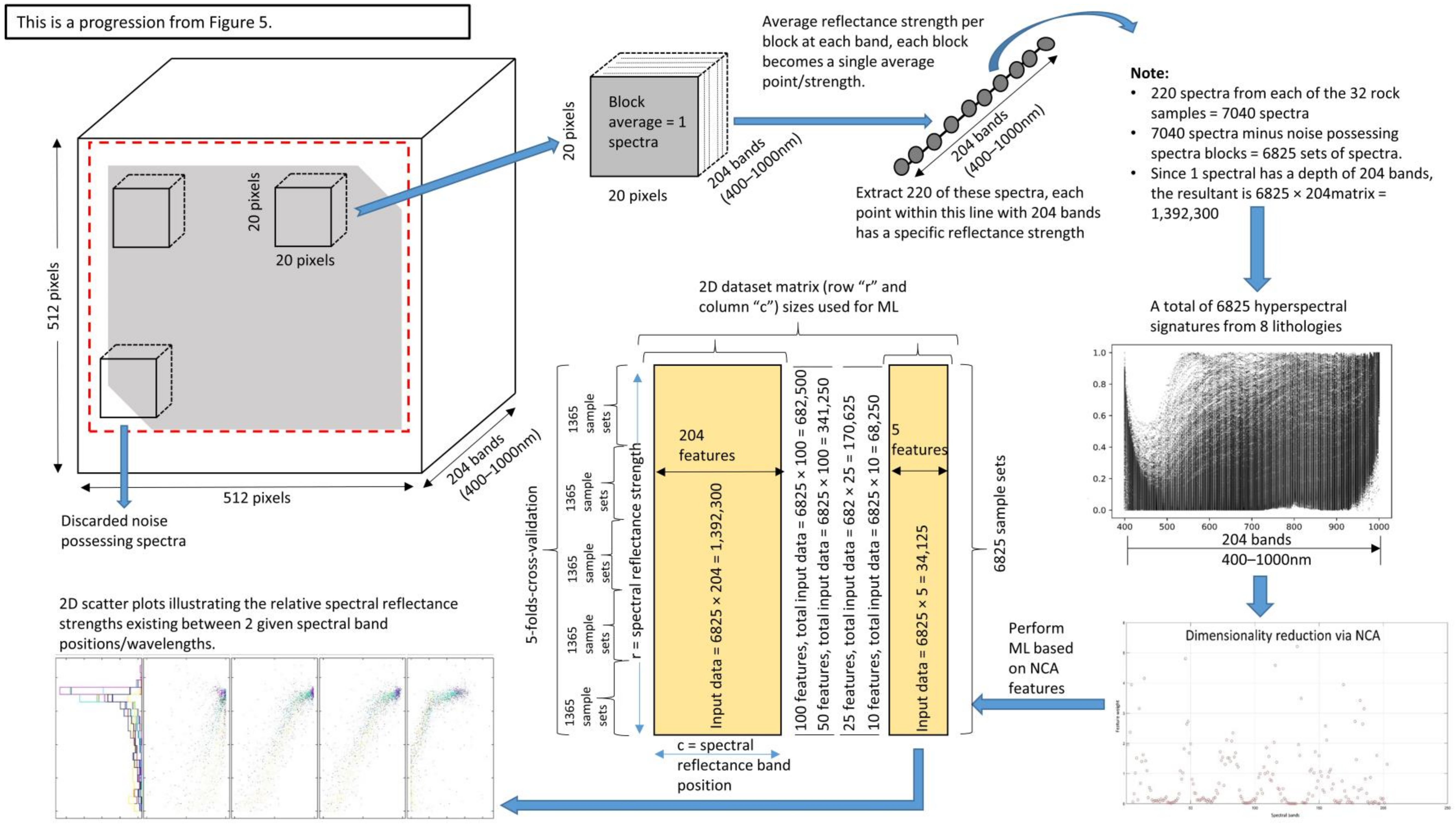
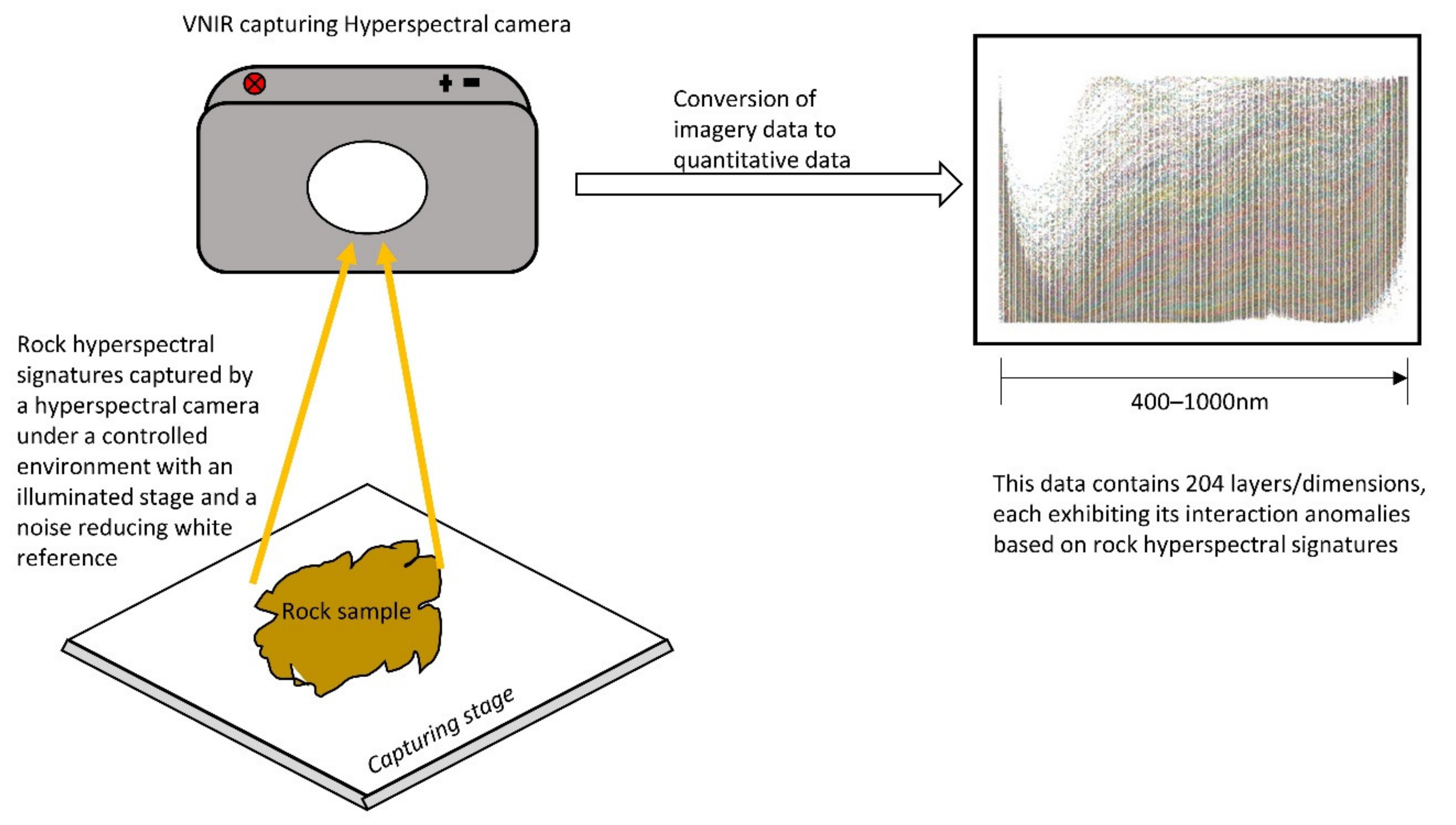
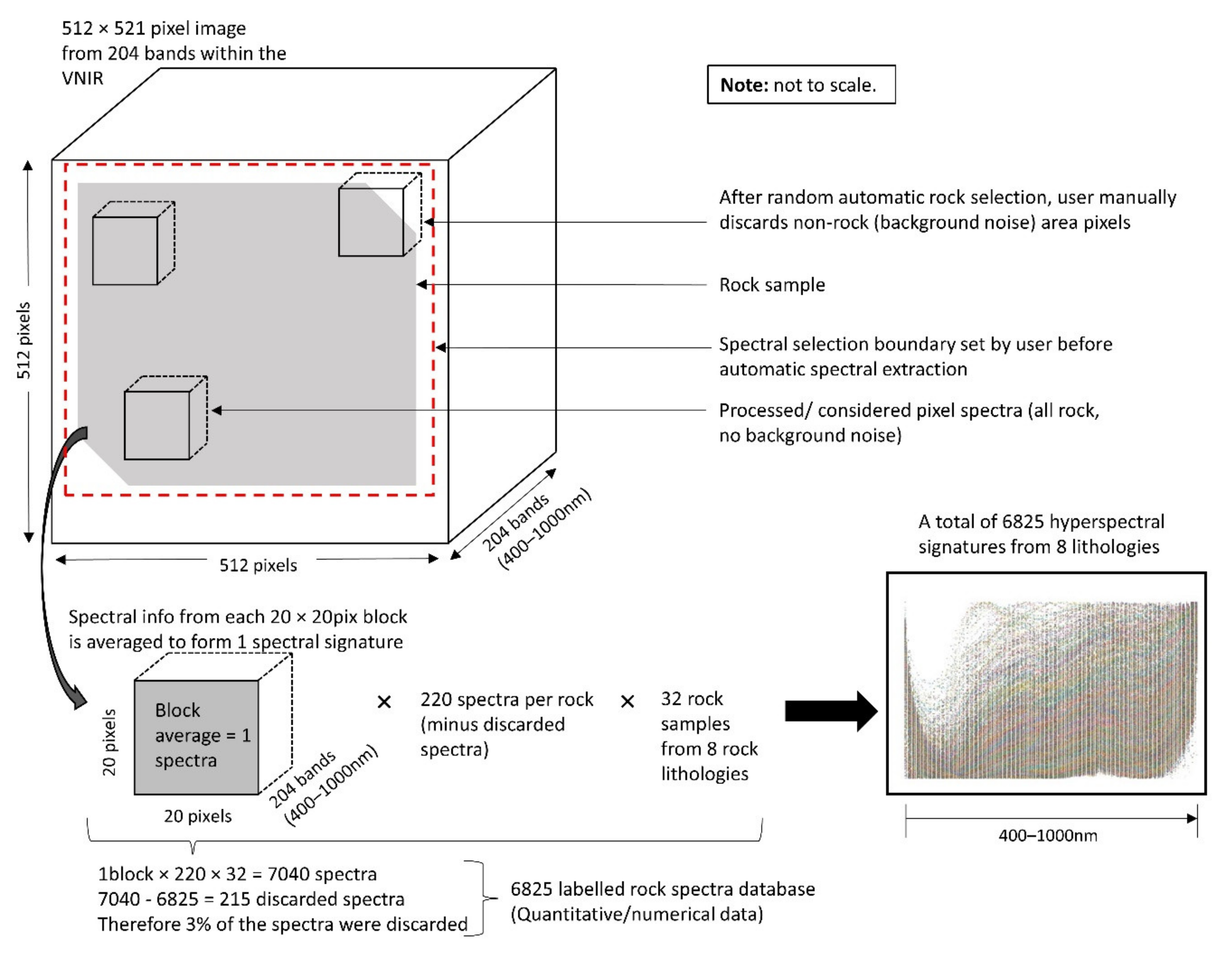
2.1. Hyperspectral Imaging

Hyperspectral imaging, as defined by researchers [2,14], refers to the collection of hundreds of pixel-scale imagery information pertaining to a subject from within the electromagnetic spectrum. The collection of such data, which in our case was within the Visible-Near-Infrared-Range (VNIR), numerically translates to the 400–1000 nm electromagnetic range [7]. Hyperspectral imaging is a graduation from multispectral imaging, meaning that within the same spectral range, hyperspectral imaging has a higher resolution, thereby facilitating the extraction of detailed spectral signatures [2,7,14]. Since its discovery, it has seen various applications in fields, such as soil sciences, hydrology, geology and the mining industry [7,15]. When an image is captured using hyperspectral camera, such as our 204 band Specim IQ capturing camera, information pertaining to the subject’s interaction with light is recorded [16]. This makes each of the 204 VNIR spectral bands receive a specific signal within each of the approximately 3 nm wide spectral bands. It should be mentioned that camera specifications may differ in terms of the number of spectral bands per spectral range provided by a certain manufacturer. This, in essence, affects the width of each spectral band, it however does not affect the underlying signatures exhibited by specific rocks and minerals.
Having said this, it is evident that analysing hyperspectral data requires sophisticated analysis software. This is because this type of data is computationally costly to analyse, due to the depth of information bands it possesses—often referred to as dimensionalities [5], hence the term dimensionality-curse [5,17,18]. To counter this phenomenon, a method referred to as DR needs to be applied to reduce or eliminate redundant information. Doing so requires a selection of the most representative spectral bands, able to distinguish rocks within our database without affecting or altering their inherent spectral signature differences.

2.2. Dimensionality Reduction

DR techniques have in the last couple of decades been a topic of interest for researchers working in computational statistics [19]. It is a key technique in data analysis, aimed at revealing expressive structures and unexpected relationships in multivariate data [20]. It should, however, be noted that, in general, it is not possible to preserve all pairwise relationships between data points in the DR process [12]. DR is used for many purposes; it is beneficial as a visualisation tool to present multivariate data in a humanly accessible form (lower dimensions). Moreover, DR can be applied as a method of feature extraction, and as a preliminary transformation applied to data, such as our rock hyperspectral database prior to the usage of other analysis tools like clustering and classification [21].
There are many criteria that can be used to sort the various methods of DR. With our objective being a classification task, the aim of our DR is, therefore, to project high-dimensional data points in a low-dimensional subspace whilst keeping most of the ‘intrinsic information’ contained in the original data preserved. This, in principle, keeps the within-class-sample compactness and between class-sample distinguishability [22]. The success of which means that low-dimensional presentation of original data may provide enough information for classification.

2.2.1. Supervised vs. Unsupervised Methods

Several DR techniques that reduce the size of the data table, while minimising loss of information have been studied, all of which can describe the essence of the primary data generated. Among these numerous methods, principal component analysis (PCA), linear discriminant analysis (LDA) and maximum margin criterion (MMC) are the most famous ones because of their simplicity and effectiveness [23]. Due to the nature of our data, we found that, geometrically, feature extractors based on maximum margin criterion (MMC) maximise the (average) margin between classes after dimensionality reduction. This would not improve our research as our goal is to use machine learning for this task [23]. On the other hand, the linear discriminant analysis (LDA) method operates by finding a linear combination of input features. However, the performance of LDA is degraded when encountering limited available low dimensional spaces and singularity problems, which is one of the disadvantages of LDA [23]. Lastly, PCA is a linear dimensionality reduction technique that transforms a set of correlated variables into a smaller number of uncorrelated variables called principal components, while retaining as much of the variation in the original dataset as possible [23,24,25].
In addition, sometimes the performance of these methods is limited, as these methods are often unsupervised. Therefore, these methods only use the global structure of the sample, while ignoring the local structure, which are extremely important in helping to improve the discrimination of the sample in the projection space. To improve on this, we have employed a supervised NCA method. The assumption being, with this supervised method, the outcome of interest informs the DR solution—this occurs because this method naturally considers the local structures and their labels [24].

2.2.2. Why Use NCA

While PCA is one of the most commonly used approaches for DR, the method does not reduce the number of variables [25]. The analyst chooses the number of components to include in analyses based on a prior defined criterion. For example, looking at the screen plot, selecting components with eigenvalues above one, or selecting the number of components that explain a prespecified proportion of the variance in the data [23]. Because PCA forces orthogonality between components, it imposes a rigid structure [23,24].
NCA, on the other hand, performs better both in terms of classification performance in the projected representation and in terms of visualisation of class separation as compared to the standard unsupervised methods. Moreover, regarding NCA, one can substantially reduce the storage, search, running and time spent on waiting costs at the test phase by forcing the learned distance metric to be low rank. This, therefore, favours its potential application in real-time field analyses [26].
NCA is a distance-based feature weighting, non-parametric supervised method, it works by automatically selecting the most significant features [11,25]. To calculate the correlation between features and target, a Mahalanobis distance-based fitness function is used. The weighting of features is carried out as follows; initial weights are assigned randomly, thereafter, weights are updated using the stochastic gradient descent or ADAM optimisation method and Mahalanobis distance-based function, hence positive weights are generated for each feature [11,25,26].
Though Goldberger et al. [11] applied their NCA algorithm for face recognition, they too mention that the NCA algorithm learns a training set distance metric, and can improve k-NN classifications, hence achieving very good performance. Koren & Carmel [20] further support the employment of an NCA model by saying it provides a linear transformation model that optimises the performance of k-NN in the learnt low-dimensional space. These said advantages influenced our desire to employ NCA in distinguishing rocks from within our rock hyperspectral database.
However, researchers [11,20,26,27] note that unlike the common PCA method, which is both convex and has an analytical solution, another key difference distinguishing the two is that NCA is a non-convex optimisation problem. This means every time one runs NCA, they may get a different solution, and like K-Means and other non-convex algorithms, it is advisable to run it more than once and take the best solution. Hence, our paper presents the best NCA bands from having run NCA multitudes of times and selected features that express themselves most frequently. Researchers [20,26] explain this by noting that this occurs as NCA components are not ordered nor dependent on the chosen target dimensions.
This, however, is not a drawback as run-times are extremely short. Moreover, once the number and specific band positions have been specified, subsequent classification tasks require significantly less storage, fewer test times, and the redundant bands are eliminated along with their datasets. These chosen components (spectral bands) are, therefore, assumed to be the most sufficient in determining the rocks within, or related to, a said database. These said sample signatures may include mine, laboratory or environmental rock spectral signatures, such as in our case.

2.3. Why Machine Learning?

Though NCA provides the opportunity to ignore redundant data-heavy bands, it does not provide any information related to the retained classification accuracy, hence the need to employ an ML algorithm(s). We use ML for multitudes of data-related tasks or problems. It has grown as a subdomain of Artificial Intelligence (AI) that comprises models capable of deriving useful information from data and utilising that information in self-learning that aids in making good classifications or predictions [7,8]. ML has gradually gained popularity, due to its accuracy and reliability [28]. Improved hardware and software components of machine vision systems have aided in building ML algorithms that process data faster and give reliable decisions in very little time [13]. Since we are dealing with a classification problem with labelled data, we employed and compared several supervised ML algorithms. Supervised learning requires learning a model from labelled training data that helps in making classification or predictions about the future data [13,29]. Supervised, in essence, indicates samples sets in which the desired output is known. In other words, the labelling of data is done to guide the machine to look for the exact desired pattern.

3. Practical Experiments

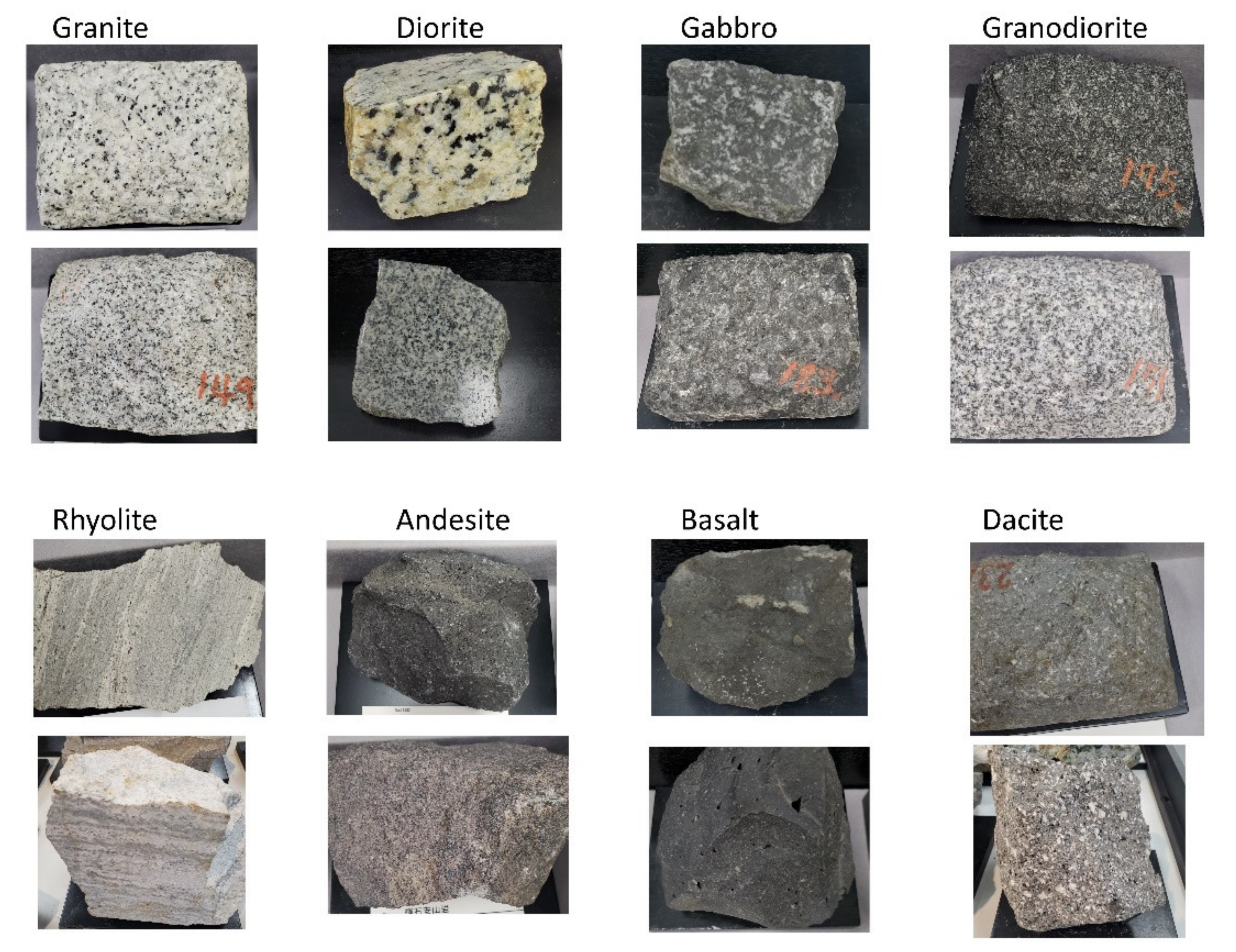
3.1. Capturing Rock Hyperspectral Signatures

To craft this proposed system, the approach involved a series of steps to be followed to get to the ultimate goal of rock classification from integrating hyperspectral imaging, NCA and ML. To develop, test and propose this system for rock engineering and classification problems, we employed 32 different igneous rocks belonging to eight rock lithologies (four samples per lithology), namely, granite, diorite, gabbro, granodiorite, rhyolite, andesite, basalt and dacite. These samples were specimens of Akita Mining Museum, each with several representative samples, such as shown in Figure 2.
To capture their spectral signatures, we used a Specim IQ hyperspectral camera (VNIR 400–1000 nm, 204 bands) to record the pixel-by-pixel signatures from rocks; the main components of the spectral data extraction setup are illustrated in Figure 3. As van der Meer [3] has pointed out, gathering this data entails standardising the spectral signature recording process. This was done by initialising the camera with a white reference board (provided by the manufacturer, Specim), the purpose of which is to filter out the noise and verify subsequent data is recorded under the same standardised conditions. The experimental setup utilises tungsten-halogen lamps to illuminate the stage as they have high output capabilities throughout the VNIR, which coincides with the camera capturing range.
Having captured the depth possessing, high dimensionality hyperspectral imagery data of all rocks, this data is then converted to numerical data using hyperspectral analysing software. Converting to numerical data entails the extraction of spectra from specific pixel blocks. This is performed after having assigned a data extraction area to allow automatic selection of pixel blocks with spectra to be considered for analysis (Figure 4). Since the Specim IQ camera acquires images of 512 × 512 pixels from 204 bands, the software randomly and automatically extracts 20 × 20-pixel information from these 204 band images (Figure 4 and Figure A1). Meaning, each spectrum is an average of the spectral reflectance information from a 20 × 20-pixels (400 pixels) area; hence, each block becomes an average spectral strength with a depth of 204 bands (wavelength). The selection area boundaries are set by the user to ensure the software extracts only relevant data.
To extract 100% of the captured image spatial area of the 512 × 512 pixels = 262,144 total pixels, a total of approximately 655 spectra (the exact number is 655.36 pixels), each with a spatial area of 20 × 20pixels = 400 pixels would have to be extracted. This is derived from dividing 262,144 pixels by 400 pixels to get 655. However, since the spectral extractor used in this study extracts 220 pixels per image, this results in approximately 30% [262,144/(220 × 400)] of the image area being used for analysis. This 30% (made up of 220 spectra minus manual elimination of non-rock spectra) of the extracted whole image area, however, can be placed anywhere on the image area using the spectral extraction boundary controlled by the user. Therefore, should a perfect 88,000 pixels (220 × 20 × 20) area be defined by the user, 100% of the selected rock spectral information without background noise (see Figure 2 and Figure 4) would be extracted. However, this was not the case in this study, as the extraction boundaries were randomly set judging from the area in which actual rock resides within each image.
Performing manual elimination (by the user) of unwanted spectra from the automatically extracted (by the software) 220 results in a lesser number of extracted spectra than the initial 220. As a result, from the 32 rock samples, we now have a total of 6825 [(220 spectra × 32 samples) minus unwanted background noise)] viable representative spectra from eight rock lithologies, each with a 204-band depth having been extracted for analysis. This, in essence, means the quantitative dataset has a matrix of size 204 × 6825 = 1,392,300 spectral information, which is used as input data in subsequent procedures. This data goes through a preprocessing stage where each dataset is assigned a relevant label; hence, a hyperspectral rock database was built based on the eight igneous rock lithologies. It should be noted that this process can be performed on any rocks, minerals or the combination or which. The choice or type of data used to develop a database depends entirely on the purpose in which rock or mineral classification is intended to be based upon. This, as a result, enables the AI coupled system to be highly specialised in classifying that which is within or related to the database.

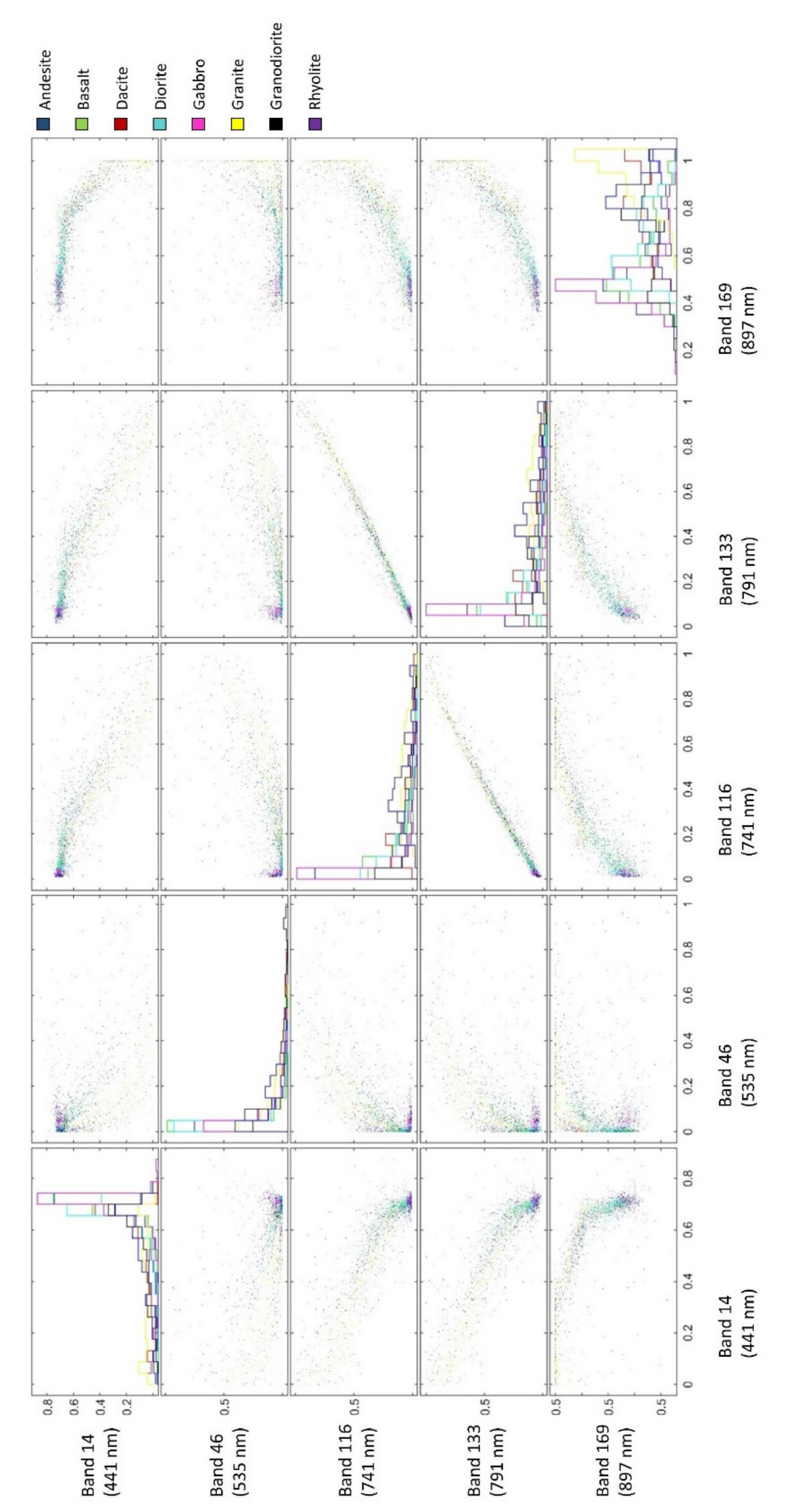
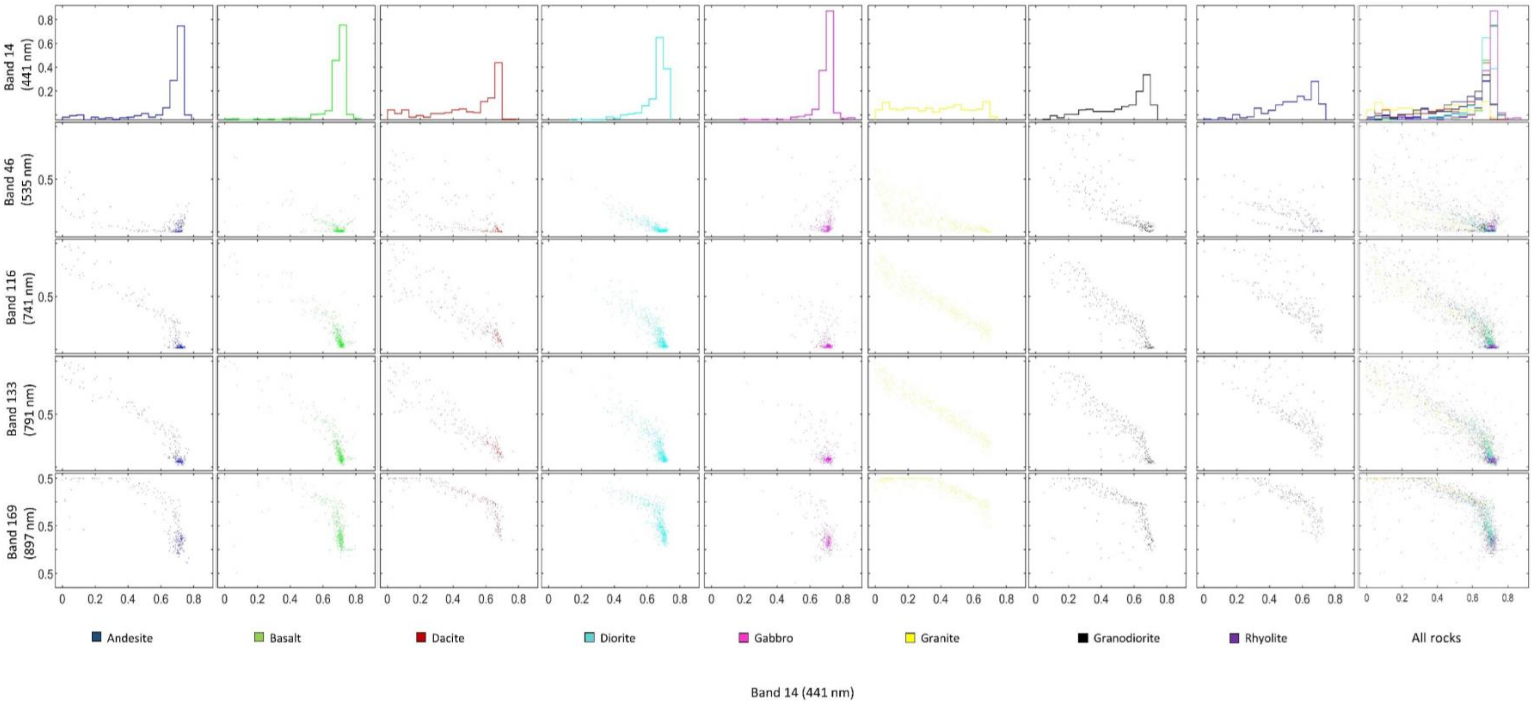
3.2. Selecting the Appropriate Feature Bands

As previously mentioned in Section 2.2, the common problem that may arise during a DR process is to define how many features to select for analysis. This is often dictated by the purpose of employing such a DR method. In this paper, based on the currently available industry produced spectral imaging devices, such as the ‘DJI P4 multispectral drone’ used in agricultural applications and environmental monitoring, our objective was to identify the appropriate rock classifying multispectral bands. From these bands, it would then be easier to develop a UAV drone-mountable multispectral sensing camera specialised in classifying rocks and minerals.
To achieve this, we convert heavy hyperspectral imagery classification data to less heavy multispectral classification data to meet weight restrictions, industry standards and production costs of developing such a device. This conversion is performed in consideration of the rocks and/or minerals from which subsequent multispectral data collection, such as from a UAV drone-mounted multispectral camera, is to be recorded and classified for a plethora of rock engineering purposes.
Transitioning from high dimensional hyperspectral to low dimensional multispectral data is not without challenges. The selection of a suitable method according to the type of data is a big issue that often needs to be addressed. It is essential to find a suitable mechanism to attain the highest level of accuracy when comparing the outputs of different DR techniques. Since it is well documented that supervised methods generally outperform unsupervised methods, we employed the NCA DR technique as it is a supervised and highly acclaimed method. As a way of determining the significance of employing the 204 spectral bands with all ‘redundant features’, we used our NCA algorithm to eliminate and record the attainable output accuracies in classifying the rocks. This was based on the full 204 feature bands, down to 100, 50, 25, 10, and finally, the current UAV drone-mountable multispectral 5-band feature classification bands. NCA DR eliminates redundant information by assigning each dimensionality from within the hyperspectral signatures a feature weight.
As [11,25,26,27] researchers have mentioned before, finding the relevant and important features is a problematic task. It entails domain knowledge, and human expertise to extract the most relevant features for future processing and selection of ML models for classification [8,13,28,29]. Employing NCA, however, makes this process easier as the algorithm assigns feature weights to each of the dimensions, thereby highlighting the most relevant features/bands for such a database. Having employed NCA to select the most relevant features that contribute most to the prediction (dependent) variable, the final step entails exporting the selected features into an ML model. The model is then trained, thereafter, we can determine the classification capabilities based solely on these feature bands.

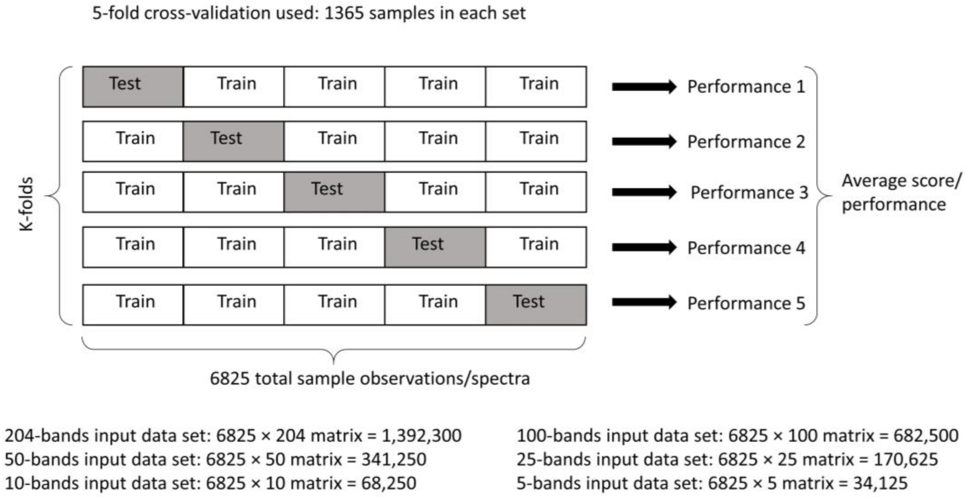
3.3. Post-NCA Classification via ML

To commence with the post-NCA classification task, we begin by preprocessing our data based on the number of spectral bands intended to be used in the rock and mineral classification task. For the initial training and classification, 100% of all the 204 spectral band signature data is employed for classification—this acts as a control task. Thereafter, depending on NCA feature weights, only the high-feature-weight possessing spectral bands are employed in succeeding classifications, which in essence means discarding the rest of the data that is deemed redundant. By doing this, we decrease data storage costs, as well as take a step towards developing a field applicable multispectral band camera. The classification was performed for 204-bands, 100, 50, 25, 10 and 5-bands using various ML models, thereby allowing for classification accuracy checks for the various band reductions.

4. Experimental and Analytical Results

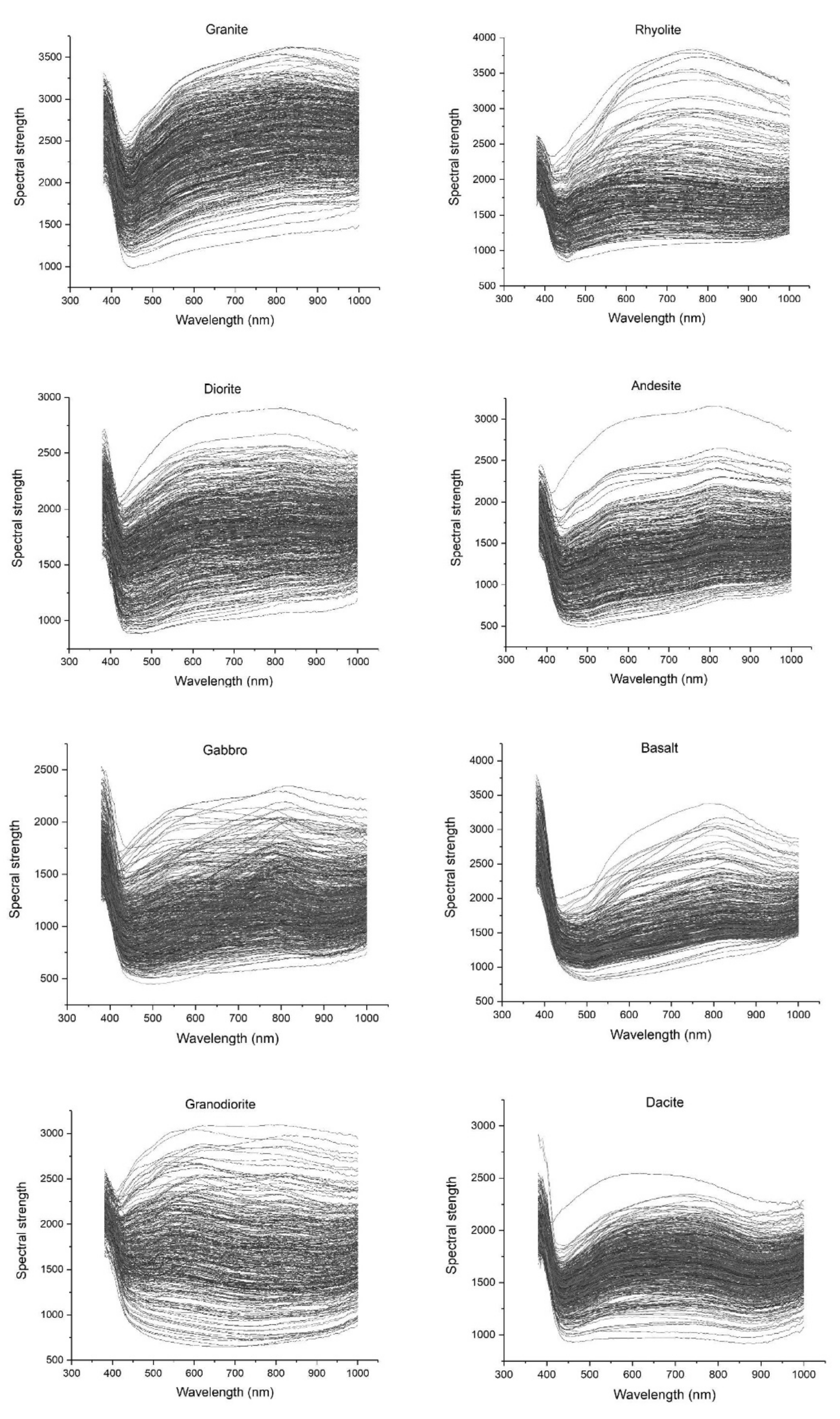
4.1. Findings Based on Hyperspectral Imaging

As a way of visualising the characteristic rock and light interactions at a pixel level from within the VNIR, Figure 5 hyperspectral signatures are typical illustrations used to visualise these inherent reflectance signatures. Each anomaly represents a given 20 × 20 pixels block as an average spectral reflectance strength from the image scene. Based on Figure 5, one can appreciate the differences in spectral reflectance strength signatures attainable from different pixels within the same hyperspectral image. Moreover, the way different rock sample variants of the same rock exhibit different signatures combined to form hyperspectral signatures, hence, each of the eight rock lithologies shows dispersed hyperspectral signatures. Taylor [30] employed VNIR spectroscopy on their ‘Mineral and Lithology Mapping of Drill Core Pulps’ problem and concluded that spectrometry, like XRD, provides an evaluation of quantitative mineralogy that is very reliable. Hence, we are confident in hyperspectral imaging is very useful in our rock identification problem, as has been hypothesised. We see these inherent differences in the spectral signatures exhibited by the rocks in our database (Figure 5).
Patterns can be drawn from hyperspectral signatures, enabling one to distinguish individual rocks and/or minerals. However, it is difficult to extract a certain anomaly from each of the eight hyperspectral rock signatures and deem it the most representative spectral signature of a particular rock and/or mineral. This can be said when for example, examining the general spectral patterns of granite with those of diorite. Their anomaly shapes seem rather similar in terms of resembling ‘check marks’, with some of them displaying comparable reflectance intensities even; the same can be said when comparing gabbro signatures with those of andesite (Figure 5). Having seen the advantages and disadvantages of hyperspectral signatures employed as a means for rock and/or mineral classification, one can acknowledge that there is a need to employ a method by which significant data is given priority over redundant data. This allows for better comparisons and distinguishability of rocks and/or minerals via their spectral signatures, which is where NCA improves on this method of rock discrimination.

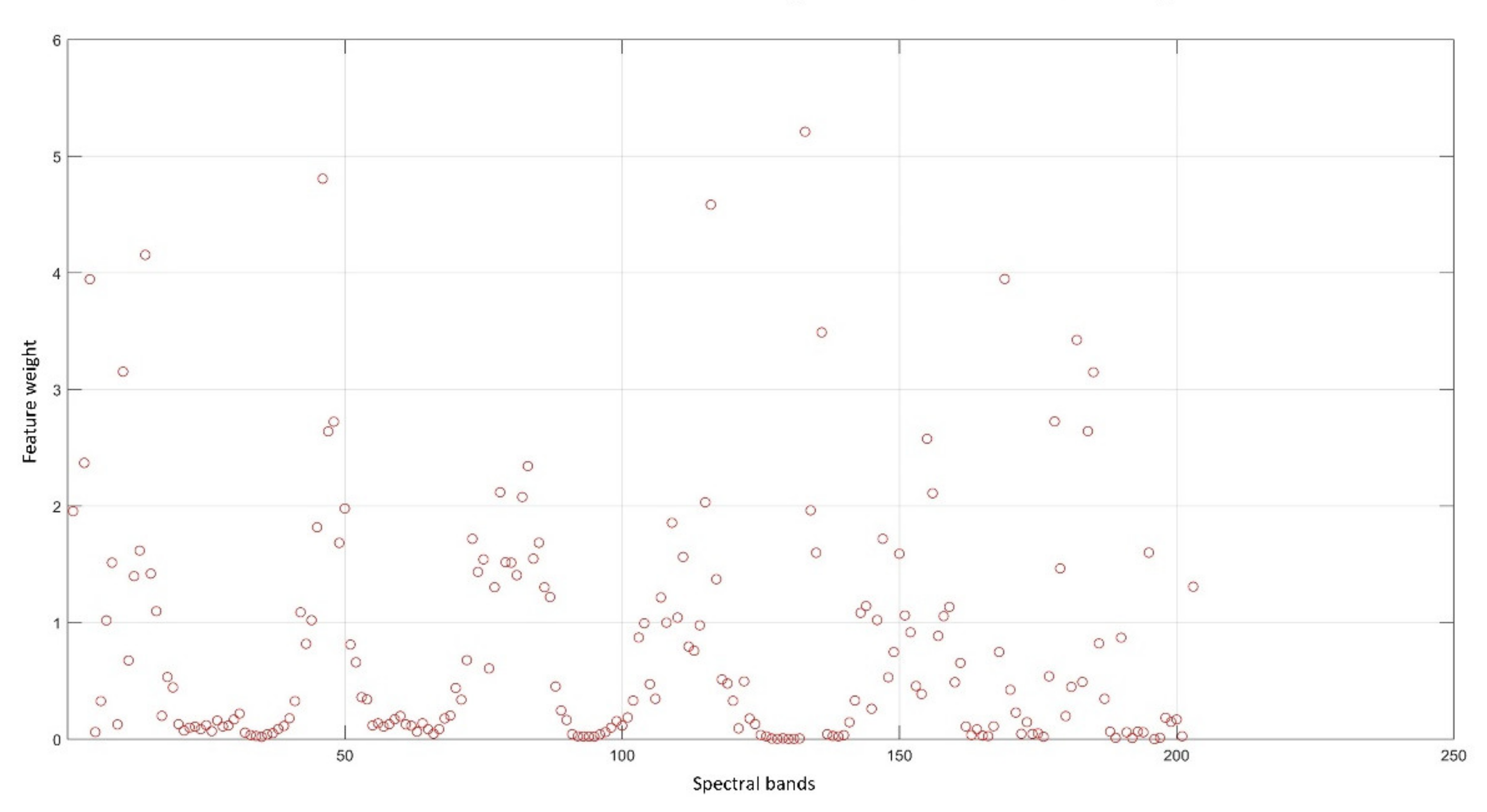
4.2. Findings Based on NCA

NCA is a method that seeks to identify and down-scale global unwanted variability within the data. The method changes the feature space used for data representation by a global linear transformation which assigns large weights to relevant dimensions, which are the most discriminatory spectral bands. Consequently, low weights are assigned to irrelevant dimensions, which we can, thus, refer to as less discriminatory spectral bands [26]. These relevant dimensions are estimated using a subset of points that are known to belong to the same although unknown class, also referred to as chunklets [31]. These chunklets are obtained from equivalence relations by applying a transitive closure within the algorithm. This transformation is, therefore, intended to reduce clutter, so that in the new feature space, the inherent structure of the data can be more easily unravelled [31,32].
Based on Figure 6, our NCA algorithm flawlessly reduced the dimensionality space of the hyperspectral signatures. We are, therefore, able to compare the different projection graphs of each of the 5-bands against one another in 2D spaces, hence mapping or visualising the manner in which the rocks plot at these chosen high classification dimensionalities. Results from the NCA algorithm in Figure 6 show that there are multitudes of spectral bands which one would refer to as relevant as they possess a substantial feature weight relative to the rest. Depending on the computational resources an entity or individual possesses, the number of spectral bands one desires to employ for future classifications having done away with redundant bands, is upon the user. Having said this, we used Figure 6 to select the most rated bands as we can indeed see the redundancy in some of the feature bands.
As stated in Section 1 and Section 3, our intended use of the most representative feature bands requires 5-bands which, according to Figure 6, are located at positions 14, 46, 116, 133 and 169 from the 204 feature bands of the VNIR. From these selected feature band positions, we can then convert these positions into electromagnetic wavelength bands. Doing so, we get 441 nm, 535 nm, 741 nm, 791 nm and 897 nm as the most discriminatory spectral bands for our rock database. It should be noted that, considering each of these spectral bands are approximately 3 nm wide, a system designed to classify rocks based on these five spectral bands would have an error of +/−3 nm, as stated in Section 2.1. Having said this, we can safely say our NCA algorithm flawlessly assigns feature weights to high dimensionality hyperspectral data. This allows the user to select the number of spectral bands they wish to employ based on NCA assigned feature weights.
DR is the transformation of data from a high-dimensional space into a low-dimensional space so that the low-dimensional representation retains some meaningful properties of the original data, ideally close to its intrinsic dimension. From this statement and having selected the now five multispectral bands to employ in future classification problems related to our data, our NCA breaks down the hyperspectral signatures. This allows for visualisation in 2D spaces whose X and Y planes are the NCA-defined spectral bands with the highest feature weights, as shown in Figure 7.
It should be noted that there are numerous ways in which these (Figure 7) dimensionally reduced band-by-band projections can be interpreted. Starting with the relative reflectance spectral strength scatter plots (normalised to 1), where each point represents the relative reflectance spectral strength of each rock sample’s previously extracted 20 × 20 pixels averages. The area within which every point plot within the scatter plots is governed by the relative spectral strength between its (previously extracted 20 × 20 block averages) spectral reflectance strength within its respective spectral band (for example, band 14), in relation to the other band (hence 2D), as well as in relation to the other seven rocks (eight in total). Having said this, the point with the highest relative spectral reflectance strength in these three categories (respective band, other band and other rocks) would plot at the right most region of the scatter plot. Having plotted these points, the relative frequency histogram sums and summarises the frequency densities of the points from 4 scatter plots into 1. Since these histograms are also relative, the most densely populated rock points are normalised to 1. From interpreting these relative scatter and histogram plots, we can assess the spectral reflectance strengths of rocks in lower, dimensionality reduced, 2D planes.
Here, is an example of interpretations deducible from Figure 7 where band 14 occupies the x-axis, and bands 46, 116, 133 and 169 occupy the y-axis. From band 14′s histogram (left most), we can make the following assumptions based on the number of rock spectral reflectance strength points summarising the scatter plots directly below it. Gabbro has the highest relative density of points (hence, the highest peak), meaning this rock has the highest concentration of points located within the further right small patch area of band 14. This is supported by the four scatter plot projections at bands 46, 116, 133 and 169, where we can see a similar dense cluster of gabbro data points (pink colour) located at this said location of the relative scatter plot projections (Figure 7 and Figure A2). Within the same patch of area, we see that the next densely populated points belong to basalt and andesite, where basalt shows a slight edge over andesite. Below these point frequency densities, we find diorite, followed by rhyolite, granodiorite, granite and dacite as the least dense.
However, we see a difference in the density of points for the histogram bar on the immediate left to the previously described. The frequency of points starts from diorite as the most densely populated within this small area. This is followed by basalt, dacite, gabbro, granodiorite, a tie between andesite and rhyolite, and granite as the least dense. Within the same band 14 projection against other bands, we can see a relatively equal frequency density of data points within the first half (left to middle) of the projection for seven rocks. This is with the exception of granite, which has a higher density of points within this wide area. Therefore, we can make similar assessments of data points for the 46, 116, 133 and 169 band, as the x-axis and draw different patterns based on the frequency and location of rock relative reflectance strength points. Having said this, we can safely say, based on Figure 7 and Figure A2 relative scatter and frequency histograms—thus, we can make predictions on future rock identification problems related to those of our study.
Hence, should new data, related to our rock database with similar multispectral bands (441 nm, 535 nm, 741 nm, 791 nm and 897 nm), be introduced, we expect such data to exhibit similar patterns as the rocks we have assessed. This may be in terms of relative frequency density relationships, or areas within which such rock relative reflectance spectral strength points are expected to exist. From these density histograms and scatter plots, we can make one more assumption. The more the frequency of data points exist within a small area, the easier it is to identify with a naked eye such rock relative points based on the scatter plots. The opposite is true for scattered data points. As much as NCA can reduce dimensionality, visual rock identification based on Figure 7 and Figure A2 patterns alone is time-consuming and prone to some human error. Hence, there is a need to employ objective ML models which can draw patterns faster and accurately. Moreover, ML models give feedback with regards to the best rock delineation strategies.

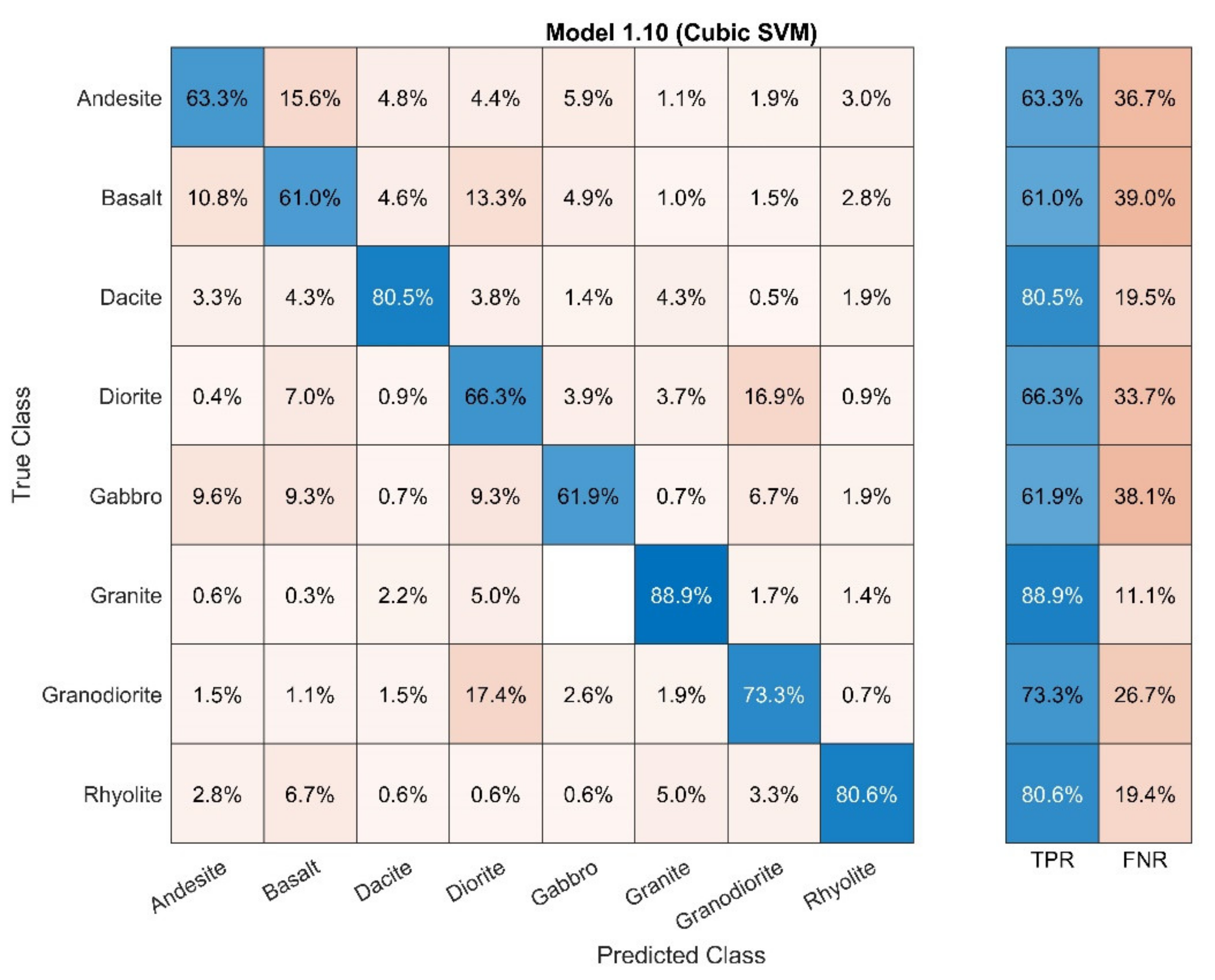
4.3. Classification with ML, Post-NCA

Supervised Learning uses an algorithm that requires external help. The provided input database is automatically separated into training and testing datasets. The output variable is predicted or classified from the training database. Algorithms try to learn some shapes during training of the database and implement these learnt patterns to the testing database, which provides results in relation to the learnt patterns [13,28,29]. From these output results, we can evaluate the performance of each algorithm.
As shown in Figure 8, a 5-folds-cross-validation (6825 divided 5) was used to process the data at all times, resulting in 1365 (Figure A1) samples (including all eight rock lithologies) being used in each set. This ensures that every observation set (with each of the eight rocks contributing) from the original dataset has the chance of appearing in training and test sets as the ultimate goal is to classify entire rocks (Figure 8). This method generally results in a less biased model compared to other methods, it is said to be one of the best approaches whenever there is a limited amount of input data [29]. Since the number of samples is 6825 (rows), it does not reduce, only the number of bands/features reduces (columns, from 204 down to 5). Each row represents the spectral reflectance strength of each rock signature, whilst each column represents the position of the wavelength band from which the spectral strengths have been extracted, hence forming a 2D matrix. As a result, a breakdown of the input dataset matrices is as follows; for 204 bands (full database), input dataset is 204 (columns) × 6825 (rows) matrix = 1,392,300; for 100 bands, input dataset is 100 × 6825 matrix = 682,500; for 50 bands, input dataset is 50 × 6825 matrix = 341,250; for 25 bands, input dataset is 25 × 6825 matrix = 170,625; for 10 bands, input dataset is 10 × 6825 matrix = 68,250; for five bands, input dataset is 5 × 6825 matrix = 34,125.
Using MATLAB R2020b classification learner Machine Learning toolbox, we assessed multiple ML algorithms and combined the best five classification performers in terms of training, average per class precision, and time taken to train the algorithm. These attributes are said to be the most important classification evaluation criteria. Moreover, these attributes govern industrial applicability, and the overall viability of the algorithm. Table 1 is a compilation of the top-performing ML algorithms per given number of selected spectral bands from the pre-DR 204 spectral bands, down to 100, 50, 25, 10 and our intended goal of five spectral bands. It demonstrates the differences in classification based on bands with the most feature weights. Results from the ML models in Table 1 show that the highest performing model in all pre- and postclassifications was Cubic Support Vector Machine (SVM).
A similar approach was applied by Galdames et al. [4] where they performed a feature selection from 2424 spectral channels to 73 spectral channels. Their study employed colour images, a VNIR sensor, as well as a SWIR (900–2500 nm) sensor. They achieved a classification performance of 99.73% using Conditional Mutual Information Maximisation to select their most important features. Considering the tools and number of bands selected at the most intrinsic bands, we would argue our methods achieves more for less. On the other hand, Mei et al. [33] employed Unsupervised Spatial-Spectral Feature Learning by 3D Convolutional Autoencoder for Hyperspectral Classification. Though with high classification capabilities, we believe this method is computationally taxing as convolutional neural networks are known to require a lot of training data and times, making CNNs invalid in our five feature bands quest.
From the results compiled in Table 1, we can appreciate the differences in accuracies acquired and elapsed times when training our ML models before and after DR. This confirms our hypothesis, which stated that with NCA, ML will maintain rapid run times and good accuracies, while maintaining without compromise, the fundamental differences in the hyperspectral signatures of rocks within our database. Global accuracy refers to the validation accuracy acquired during training. Average per-class precision refers to the individual rock classification sum averages in testing the models. Lastly, training time refers to elapsed time in training the models to classify the rocks based on the number of spectral band datasets.
As our goal was to reduce the number of hyperspectral bands to five multispectral bands capable of distinguishing rocks at a substantial, industry applicable accuracy, we assessed the highest performing Cubic SVM ML model for the 5-band classification. The results are presented in Figure 9. To assess the viability of this Cubic SVM model, Figure 9 presents two performance metrics. The first is True Positive Rates (TPR), defined as the probability that an actual positive will test positive (Equation (1)). The second is False Negative Rates (FNR), defined as the probability that a true positive will be missed by the test (Equation (2)). Both variables are highly viable in assessing the capability of the ML model in classifying each rock. Another assessment that can be drawn from Figure 9 confusion matrix is the average per-class precision of 72%. This is substantial considering the magnitude of the DR from 100% of that hyperspectral data (204-bands) to approximately 2.5% (5-bands), which we now refer to as multispectral data. We have, therefore, determined an applicable classification model for this particular problem. In addition to this, we gained a reduction in computational costs and storage requirements, ease of data management, ease of data application and visualisation, and most importantly, viability in rapid field applications.
In addition to the above-given assessment, Figure 9 illustrates the in depth classification capabilities of the ML algorithm post-DR for each class of rocks employed in this study. From the Figure 9 confusion matrix, 63.3% of the initial input andesite datasets (for 5-bands) were correctly (TPR) classified as andesite. On the other hand, the remaining 36.7% (FNR) was incorrectly classified as basalt (15.6%), dacite (4.8%), diorite (4.4%), gabbro (5.9%), granite (1.1%), granodiorite (1.9%), and rhyolite (3.0). Similar assessments can be made for all rocks, resulting in different ratios of both TPR and FNR. Comparing Figure 7 and Figure A2 and nine results, we can make the following assumptions; the flatter the relative frequency histograms (Figure 7 and Figure A2), the higher the prediction precision (Figure 9), hence granite has the highest ML prediction precision. On the other hand, the steeper the relative frequency histograms (Figure 7 and Figure A2), the lower the ML prediction precision (Figure 9), hence basalt and gabbro have lower ML prediction precision outcomes. By developing algorithms on a particular type of rock, it is possible to improve any of the Figure 9 results to favour that specific rock, mineral or environmental phenomenon of interest. This thereby makes this system highly applicable in a magnitude of highly specialised classification problems. Doing so simply requires importing the most discriminative hyperspectral bands of any particular rock, mineral, or phenomenon, and giving them priority over other spectral bands, hence improving their succeeding ML classification outputs. However, since the goal of this paper was to classify eight igneous rock lithologies as a collective based on five multispectral bands, our system was not preprogrammed to be biased towards any of the eight igneous rock lithologies, but rather used the data as is, hence the true/unmodified results.
True Positive Rates (TPR):
TPR = (TP/TP + FN) × 100
False Negative Rates (FNR):
FNR = (FN/FN + TP) × 100
where FN is false negatives, and TP is true positives.

5. Significance of Proposed System

Therefore, given our findings, we can confirm that our proposed system, which consists of DR of rock hyperspectral data and subsequently employing specific discriminant features for our igneous rock database, performs extremely well. This, in essence, means for rock engineering, problems requiring discrimination of rocks, minerals, soils and other environmental phenomena based on their spectral signatures can indeed employ this system. By setting desired attributes founded on preknowledge of a site, such as types of rocks present within a mine site, rocks transported via a conveyer belt, or the general mapping of the environment, it is possible to maximise data collection. Based on specific multispectral bands, we can eliminate unnecessary storage, processing or classification costs associated with massive data.
With our integrated system, here are several optimisations we were able to achieve:
  • Through DR, we can reduce the storage capacity required to store and handle a database, thereby reducing storage costs as we have proven there is no need to collect, store and process redundant data;
  • With DR, we were able to break down hyperspectral signature data into different dimensionalities, hence the ability to plot such data in 2D planes, which as a result allows for easy visual assessment;
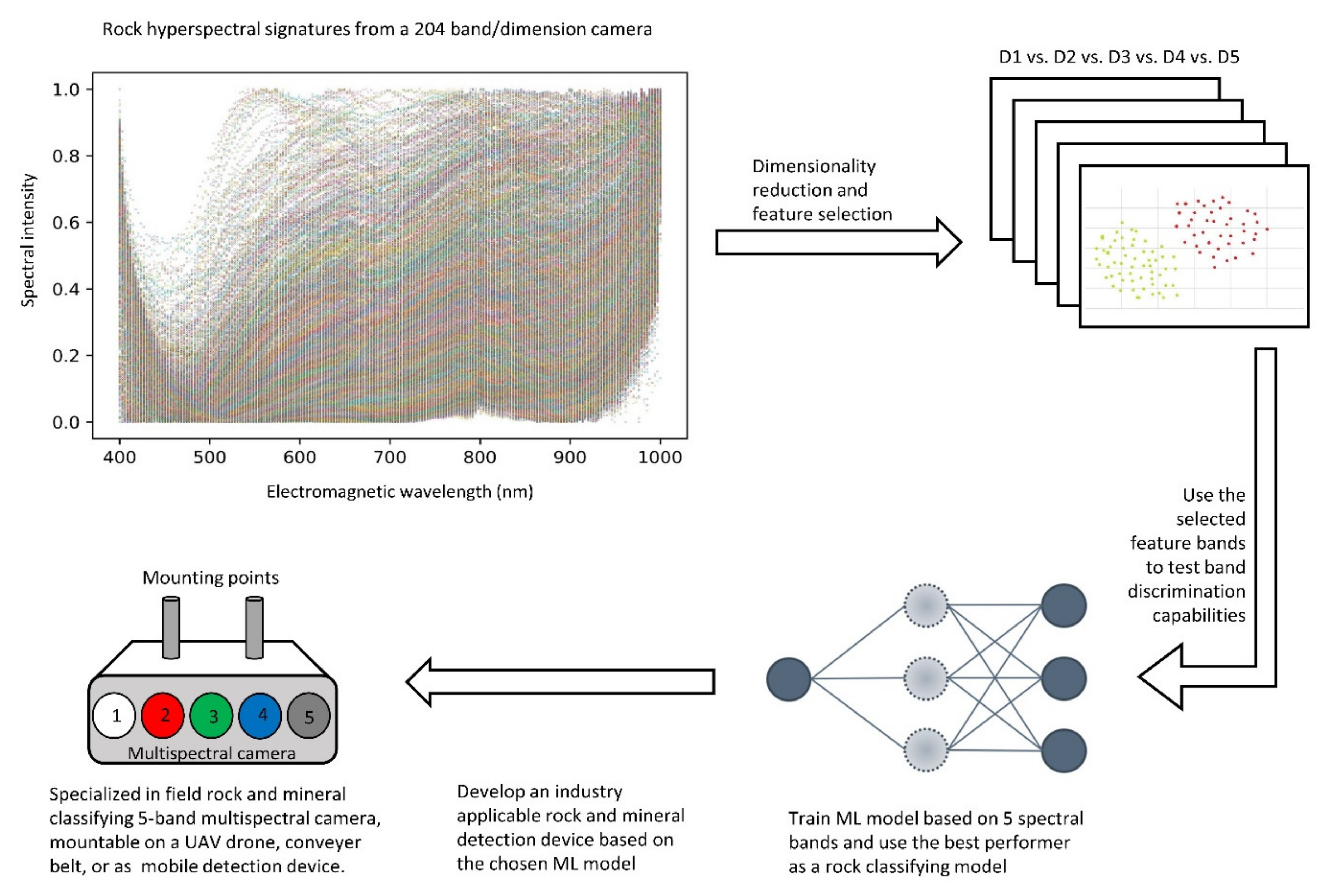
  • As proven with post-NCA specialised multispectral imaging, we can attain respectable classification accuracies. This proves that multispectral imaging is a good enough option as it can be programmed to be highly specialised, costs less, has lower operation costs, has the flexibility of being applied in specialised multispectral imaging, such as on a UAV drone. Having said this, it is important to note that samples used in this study were clean and manually prepared before analysis, which is not the state in which rocks are found in the field, due to dirt and other matter. Therefore, classification accuracy variations in our envisioned identification of these rocks in the field, compared to the study’s attained results, are likely to exist;
  • Through ML, we can analyse and classify multispectral signatures produced by rocks and minerals with high accuracies. By finding the right model for a particular dataset, subsequent related data is relatively easier to classify as the training data always assists the model in future predictions as proven;
  • With our proposed combined system, we have proved that any industry looking to cut spectral data (or equivalent) analysis costs whilst still retaining high classification accuracies, DR via a feature selection supervised NCA algorithm to specify the most discriminative bands, and verifying the viability of selected bands via ML, thereafter employing these 5-bands (or more, depending on application) in future specialised classifications, could potentially be the key to achieving several system design optimisations;
  • Via a post-NCA 5-band rock and mineral classification specialised multispectral camera mounted on a UVA drone, such as the ‘DJI P4 Multispectral drone used in agricultural applications’, there is a plethora of applications in which this specialised technology could find potential use. This, as a result, minimises purchase, operation and data interpretation costs as compared to a hyperspectral imaging system. This could aid in remote sensing from long distances without the need for physical presence, as well as rapid in situ assessments of the state of the environment via the UAV drone, possibilities are endless.
  • Lastly, there is potential to employ such a post-NCA specialised multispectral camera in the frequent monitoring of mine dams. This would allow quicker assessment of contaminants based on spectral signatures produced by unexpected and/or anticipated metal contaminants. Hence, we deem this proposed system viable in all mining-related stages, from exploration, operation and closure.

6. Conclusions

This paper proposes the combination and DR of hyperspectral data via NCA to multispectral imaging, coupled with ML as a method by which subsequent spectral characteristics of rocks, minerals and the environment can be performed without unnecessary processing of redundant data. With our NCA algorithm, we proved the viability of our hyperspectral data DR from 204-bands, to 100, 50, 25, 10, and finally, the industry standard 5-band multispectral dimensionality. Thus, from NCA, we can conclude that the most viable discriminative five multispectral bands viable in the classification of igneous rocks, such as granite, diorite, gabbro, granodiorite, rhyolite, andesite, basalt and dacite, are bands with the following wavelengths—441 nm, 535 nm, 741 nm, 791 nm and 897 nm. With this DR, we were able to produce 2D data plots, which provide better interpretation, visualisation and somewhat data prediction capabilities in the form band-against-band scatter plots, as well as frequency density histograms. Therefore, it can be said that by eliminating redundant features, DR can be a useful technique employable for various datasets possessing the dimensionality curse.
The proposed method flawlessly merges with several ML models. Hence, we are provided with quantitative outputs pertaining to the classification abilities of each ML model, an example being our Cubic SVM model, which outperformed all other ML models in the classification of igneous rocks in our database. This, in essence, deems the Cubic SVM ML model the most viable as it attained a global classification accuracy of 71%, and an average per-class accuracy of 72%, which is considerable given the magnitude of the DR from 204-bands to 5-bands.

Author Contributions

Conceptualisation, B.B.S. and Y.K.; Data curation, H.T.; Formal analysis, M.S.; Funding acquisition, Y.K.; Investigation, B.B.S.; Methodology, B.B.S.; Resources, F.I.; Software, N.O.; Supervision, Y.K.; Validation, Z.B.; Visualisation, M.S. and H.T.; Writing—original draft, B.B.S.; Writing—review & editing, Z.B. and Y.K. All authors have read and agreed to the published version of the manuscript.

Funding

This Work Was Supported by JSPS ‘Establishment of Research and Education Hub on Smart Mining for Sustainable Resource Development in Southern African Countries’. Grant number: JPJSCCB2018005.

Acknowledgments

This research was supported by SATREPS in collaboration between JST and JICA. We would like to express our sincere gratitude to Akita Mining Museum for permitting us to use their specimens as our research data, from which we were able to build a considerable database. Anonymous reviewers are thanked for critically reading the manuscript and suggesting substantial improvements.

Conflicts of Interest

The authors declare no conflict of interest.

Appendix A

Figure A1. Summary of rock spectral reflectance strength data accumulation and preprocessing prior to dimensionality reduction via Neighbourhood Component Analysis and Machine Learning (a continuation from Figure 5).
Minerals 11 00846 g0a1
Figure A2. Relative scatter and histogram plots of rock spectral reflectance strengths in 2D plane projections, where bands 441 nm is the x-axis, and bands 535 nm, 741 nm, 791 nm and 897 nm are the y-axis. The position of each point (spectra) is based on the relative intensities between bands, as well as between rocks.
Minerals 11 00846 g0a2

References

  1. Jia, F.; Lei, Y.; Lin, J.; Zhou, X.; Lu, N. Deep Neural Networks: A Promising Tool for Fault Characteristic Mining and Intelli-gent Diagnosis of Rotating Machinery with Massive Data. Mech. Syst. Signal Process. 2016, 72, 303–315. [Google Scholar] [CrossRef]
  2. Zhang, X.; Li, P. Lithological Mapping from Hyperspectral Data by Improved Use of Spectral Angle Mapper. Int. J. Appl. Earth Obs. Geoinf. 2014, 31, 95–109. [Google Scholar] [CrossRef]
  3. Van der Meer, F. The Effectiveness of Spectral Similarity Measures for the Analysis of Hyperspectral Imagery. Int. J. Appl. Earth Obs. Geoinf. 2006, 8, 3–17. [Google Scholar] [CrossRef]
  4. Galdames, F.J.; Perez, C.A.; Estévez, P.A.; Adams, M. Rock Lithological Classification by Hyperspectral, Range 3D and Color Images. Chemom. Intell. Lab. Syst. 2019, 189, 138–148. [Google Scholar] [CrossRef]
  5. Ruiz Hidalgo, D.; Bacca Cortés, B.; Caicedo Bravo, E. Dimensionality Reduction of Hyperspectral Images of Vegetation and Crops Based on Self-Organized Maps. Inf. Process. Agric. 2020. [Google Scholar] [CrossRef]
  6. Tong, Z.; Gao, J.; Zhang, H. Recognition, Location, Measurement, and 3D Reconstruction of Concealed Cracks Using Con-volutional Neural Networks. Constr. Build. Mater. 2017, 146, 775–787. [Google Scholar] [CrossRef]
  7. Sinaice, B.B.; Kawamura, Y.; Kim, J.; Okada, N.; Kitahara, I.; Jang, H. Application of Deep Learning Approaches in Igneous Rock Hyperspectral Imaging. In Proceedings of the 28th International Symposium on Mine Planning and Equipment Selec-tion—MPES 2019; Springer Series in Geomechanics and Geoengineering; Topal, E., Ed.; Springer International Publishing: Cham, Switzerland, 2020; pp. 228–235. [Google Scholar] [CrossRef]
  8. Sharma, N.; Sharma, R.; Jindal, N. Machine Learning and Deep Learning Applications—A Vision. Glob. Transit. Proc. 2021, 2, 24–28. [Google Scholar] [CrossRef]
  9. Asscher, Y.; Angelini, I.; Secco, M.; Parisatto, M.; Chaban, A.; Deiana, R.; Artioli, G. Mineralogical Interpretation of Multispectral Images: The Case Study of the Pigments in the Frigidarium of the Sarno Baths, Pompeii. J. Archaeol. Sci. Rep. 2021, 35, 102774. [Google Scholar] [CrossRef]
  10. Rahimi, B.; Sharifzadeh, M.; Feng, X.-T. A Comprehensive Underground Excavation Design (CUED) Methodology for Geotechnical Engineering Design of Deep Underground Mining and Tunneling. Int. J. Rock Mech. Min. Sci. 2021, 143, 104684. [Google Scholar] [CrossRef]
  11. Goldberger, J.; Roweis, S.; Hinton, G.; Salakhutdinov, R. Neighbourhood Components Analysis. 8. Available online: https://www.cs.toronto.edu/~hinton/absps/nca.pdf (accessed on 5 February 2021).
  12. Venna, J. Dimensionality Reduction for Visual Exploration of Similarity Structures. 82. Available online: https://www.researchgate.net/publication/27516587 (accessed on 23 March 2021).
  13. Saha, D.; Annamalai, M. Machine Learning Techniques for Analysis of Hyperspectral Images to Determine Quality of Food Products: A Review. Curr. Res. Food Sci. 2021, 4, 28–44. [Google Scholar] [CrossRef] [PubMed]
  14. Salles, R.D.R.; de Souza Filho, C.R.; Cudahy, T.; Vicente, L.E.; Monteiro, L.V.S. Hyperspectral Remote Sensing Applied to Uranium Exploration: A Case Study at the Mary Kathleen Metamorphic-Hydrothermal U-REE Deposit, NW, Queensland, Australia. J. Geochem. Explor. 2017, 179, 36–50. [Google Scholar] [CrossRef]
  15. Kruse, F.A. Mapping Surface Mineralogy Using Imaging Spectrometry. Geomorphology 2012, 137, 41–56. [Google Scholar] [CrossRef]
  16. Ganesh, U.K.; Kannan, S.T. Creation of Hyper Spectral Library and Lithological Discrimination of Granite Rocks Using SVCHR -1024: Lab Based Approach. J. Hyperspectral Remote. Sens. 2017, 7, 168–177. [Google Scholar]
  17. Li, Y.; Chai, Y.; Zhou, H.; Yin, H. A Novel Dimension Reduction and Dictionary Learning Framework for High-Dimensional Data Classification. Pattern Recognit. 2021, 112, 107793. [Google Scholar] [CrossRef]
  18. Li, J.; Wang, T. Dimension Reduction in Binary Response Regression: A Joint Modeling Approach. Comput. Stat. Data Anal. 2021, 156, 107131. [Google Scholar] [CrossRef]
  19. Zuniga, M.M.; Murangira, A.; Perdrizet, T. Structural Reliability Assessment through Surrogate Based Importance Sampling with Dimension Reduction. Reliab. Eng. Syst. Saf. 2021, 207, 107289. [Google Scholar] [CrossRef]
  20. Koren, Y.; Carmel, L. Robust Linear Dimensionality Reduction. IEEE Trans. Vis. Comput. Graph. 2004, 10, 459–470. [Google Scholar] [CrossRef]
  21. Bar-Hillel, A.; Hertz, T.; Shental, N.; Weinshall, D. Learning a Mahalanobis Metric from Equivalence Constraints. J. Mach. Learn. Res. 2005, 6, 937–965. [Google Scholar]
  22. Zhang, C.; Lei, Y.-K.; Zhang, S.; Yang, J.; Hu, Y. Orthogonal Discriminant Neighborhood Analysis for Tumor Classification. Soft Comput. 2016, 20, 263–271. [Google Scholar] [CrossRef]
  23. Hu, H.; Feng, D.-Z.; Chen, Q.-Y. A Novel Dimensionality Reduction Method: Similarity Order Preserving Discriminant Analysis. Signal Process. 2021, 182, 107933. [Google Scholar] [CrossRef]
  24. Kalia, V.; Walker, D.I.; Krasnodemski, K.M.; Jones, D.P.; Miller, G.W.; Kioumourtzoglou, M.-A. Unsupervised Dimen-sionality Reduction for Exposome Research. Curr. Opin. Environ. Sci. Health 2020, 15, 32–38. [Google Scholar] [CrossRef]
  25. Jiang, Z.; Li, J. High Dimensional Structural Reliability with Dimension Reduction. Struct. Saf. 2017, 69, 35–46. [Google Scholar] [CrossRef]
  26. Liu, J.; Chen, S. Discriminant Common Vecotors Versus Neighbourhood Components Analysis. 32. Image Vis. Comput. 2006, 24, 249–262. [Google Scholar] [CrossRef]
  27. Kartun-Giles, A.P.; Bianconi, G. Beyond the Clustering Coefficient: A Topological Analysis of Node Neighbourhoods in Complex Networks. Chaos Solitons Fractals X 2019, 1, 100004. [Google Scholar] [CrossRef]
  28. Gunduz, H. An Efficient Dimensionality Reduction Method Using Filter-Based Feature Selection and Variational Auto encoders on Parkinson’s Disease Classification. Biomed. Signal Process. Control 2021, 66, 102452. [Google Scholar] [CrossRef]
  29. Jain, U.; Nathani, K.; Ruban, N.; Joseph Raj, A.N.; Zhuang, Z.; Mahesh, V.G.V. Cubic SVM Classifier Based Feature Extraction and Emotion Detection from Speech Signals. In Proceedings of the 2018 International Conference on Sensor Networks and Signal (SNSP), Xi’an, China, 28–31 October 2018. [Google Scholar] [CrossRef]
  30. Taylor, G.R. Mineral and Lithology Mapping of Drill Core Pulps Using Visible and Infrared Spectrometry. Nat. Resour. Res. 2000, 9, 257–268. [Google Scholar] [CrossRef]
  31. Bar-Hillel, A.; Hertz, T.; Shental, N.; Weinshall, D. Learning Distance Functions Using Equivalence Relations. In Proceedings of the Twentieth International Conference on Machine Learning (ICML-2003), Washington, DC, USA, 21–24 August 2003; Available online: https://www.researchgate.net/publication/221344999_Learning_Distance_Functions_using_Equivalence_Relations (accessed on 23 March 2021).
  32. Ayesha, S.; Hanif, M.K.; Talib, R. Overview and Comparative Study of Dimensionality Reduction Techniques for High Dimensional Data. Inf. Technol. Control 2020, 59, 44–58. [Google Scholar] [CrossRef]
  33. Mei, S.; Ji, J.; Geng, Y.; Zhang, Z.; Li, X.; Du, Q. Unsupervised Spatial–Spectral Feature Learning by 3D Convolutional Auto-encoder for Hyperspectral Classification. IEEE Trans. Geosci. Remote. Sens. 2019, 57, 6808–6820. [Google Scholar] [CrossRef]
Figure 1. Our proposed system design, consisting of hyperspectral imaging, dimensionality reduction via Neighbourhood Component Analysis, Machine Learning classification of rocks and minerals to test system viability based on the selected features, and finally employing those features together with the ML model in developing a unmanned aerial vehicle drone-mountable multispectral camera.
Minerals 11 00846 g001
Figure 2. Images of some of the 32 rock samples from eight rock lithologies used in building our rock hyperspectral database.
Minerals 11 00846 g002
Figure 3. A hyperspectral signature capturing setup is used in collecting and building a rock and/or mineral spectral database. The curves are spectra in different spatial pixels of eight rock lithologies.
Minerals 11 00846 g003
Figure 4. Automatic random extraction of rock pixel spectra captured via a Specim IQ camera that acquires 512 × 512 pixel images from 204 bands within the Visible-Near-Infrared-Range. Extracted spectra are used to build a rock hyperspectral database.
Minerals 11 00846 g004
Figure 5. Reflectance hyperspectral signatures of eight rock lithologies employed in the construction of a hyperspectral database. Each anomaly represents the interaction between each 20 × 20 pixels 2D area with a depth of 204 bands within a rock’s hyperspectral image with light, captured via a Visible-Near-Infrared-Range hyperspectral camera.
Minerals 11 00846 g005
Figure 6. Neighbourhood Component Analysis feature selection which assigns higher weights to the most discriminatory hyperspectral bands by eliminating redundancy in data, with the top five feature-bands being 14, 46, 116, 133 and 169.
Minerals 11 00846 g006
Figure 7. Projection of complex rock hyperspectral signature data points in dimensionality reduced (via Neighbourhood Component Analysis feature selection) 2D planes showing the relative reflectance spectral strength relationships between five different spectral bands for eight rock lithologies.
Minerals 11 00846 g007
Figure 8. Database handling of training and testing sets. A 5-fold-cross-validation was used in all instances.
Minerals 11 00846 g008
Figure 9. Confusion matrix from a Cubic SVM machine learning model used in evaluating the classification viability of post dimensionality reduction spectral bands.
Minerals 11 00846 g009
Table 1. Top five machine learning classification comparisons based on predimensionality reduction from 204-bands, to postdimensionality reduction (using Neighbourhood Component Analysis) for 100, 50, 25, 10 and 5 rock spectral bands.
Number of Classification Bands Post-NCAMachine Learning AlgorithmGlobal
Accuracy (%)
Average per-Class Precision (%)Training Time (s)
204-bands 1SVM (Cubic SVM)90.790.028.7
SVM (Quadratic SVM)87.086.027.3
SVM (Linear SVM)79.176.513.8
Linear discriminant80.478.44.6
Ensemble (Subspace discriminant)81.279.341.5
100-bandsSVM (Cubic SVM)89.488.737.7
SVM (Quadratic SVM)84.783.821.8
Quadratic Discriminant77.977.51.0
SVM (Linear SVM) 76.976.05.9
Linear Discriminant76.775.61.1
50-bandsSVM (Cubic SVM)86.985.739.1
SVM (Quadratic SVM)84.382.123.2
Quadratic Discriminant79.178.91.1
SVM (Linear SVM)76.175.45.3
Ensemble (Subspace KNN) 75.275.034.9
25-bandsSVM (Cubic SVM)86.386.245.1
SVM (Quadratic SVM)83.982.628.2
SVM (Fine Gaussian SVM) 75.970.66.7
Quadratic Discriminant75.775.31.2
Ensemble (Subspace KNN)75.470.029.2
10-bandsSVM (Cubic SVM)81.080.378.2
SVM (Quadratic SVM)78.276.040.7
SVM (Fine Gaussian SVM)72.770.18.2
Ensemble (Bagged tress)71.069.819.1
Ensemble (Subspace KNN)70.670.317.9
5-bandsSVM (Cubic SVM)70.972.0182.1
Ensemble (Bagged trees)68.667.012.3
SVM (Quadratic SVM)68.465.876.7
SVM (Fine Gaussian SVM)68.466.67.5
KNN (Fine KNN)67.366.05.7
1 Predimensionality reduction.
Publisher’s Note: MDPI stays neutral with regard to jurisdictional claims in published maps and institutional affiliations.

