
Multiphysics Modeling Simulation and Optimization of Aerodynamic Drum Magnetic Separator


Abstract
:1. Introduction
2. Methods
2.1. Modeling
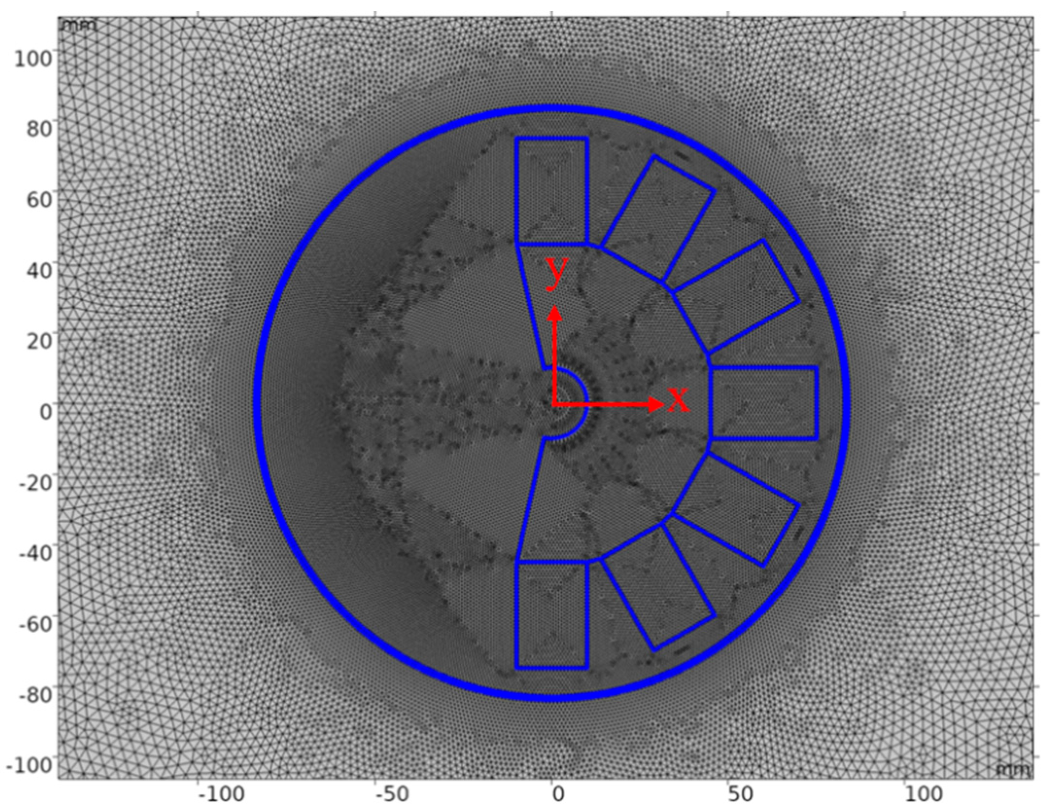
2.1.1. Structure
2.1.2. Magnetic Field
2.1.3. Flow Field
2.1.4. Particle Dynamic Tracking
2.1.5. Meshing
2.2. Verification
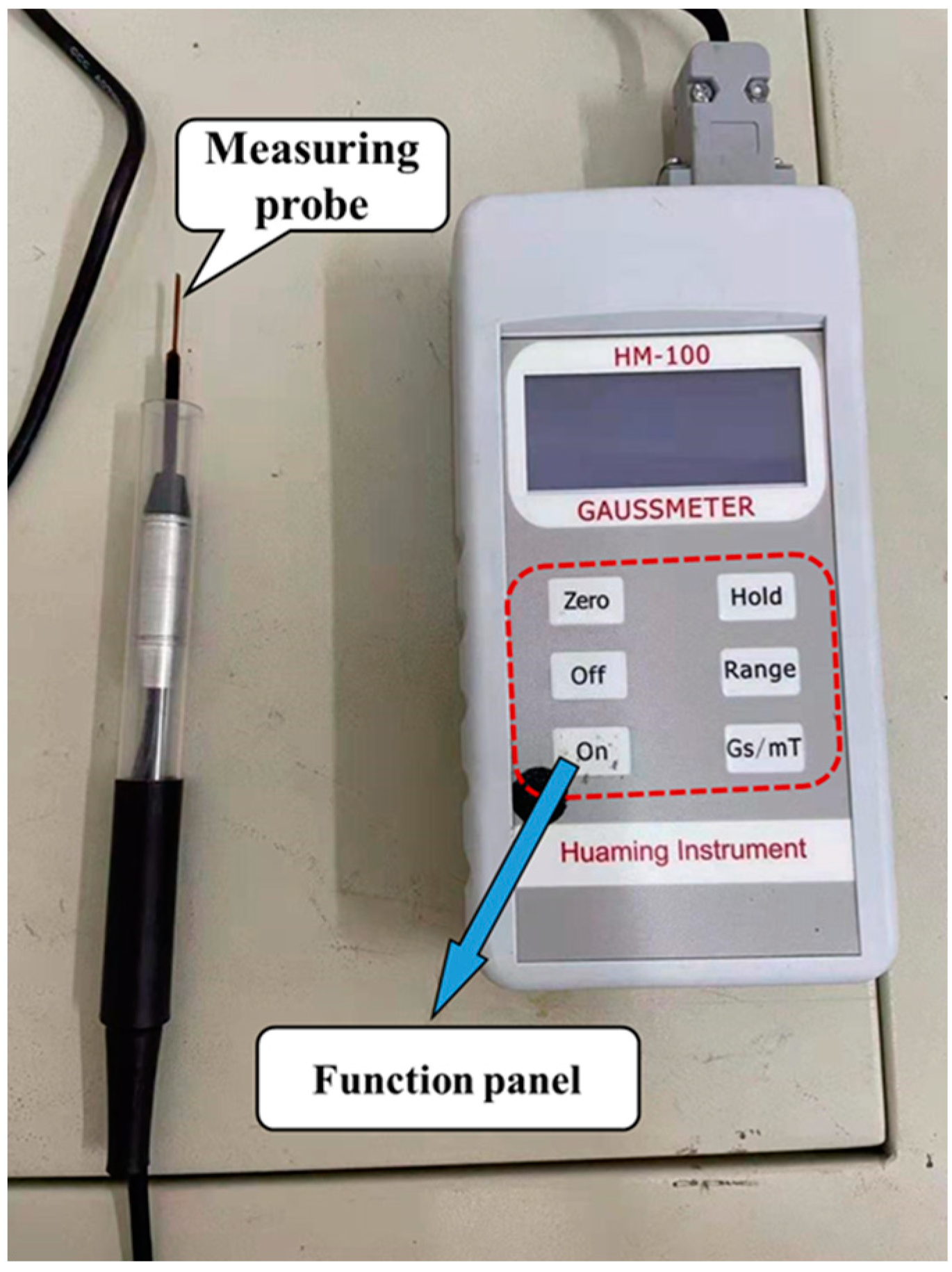
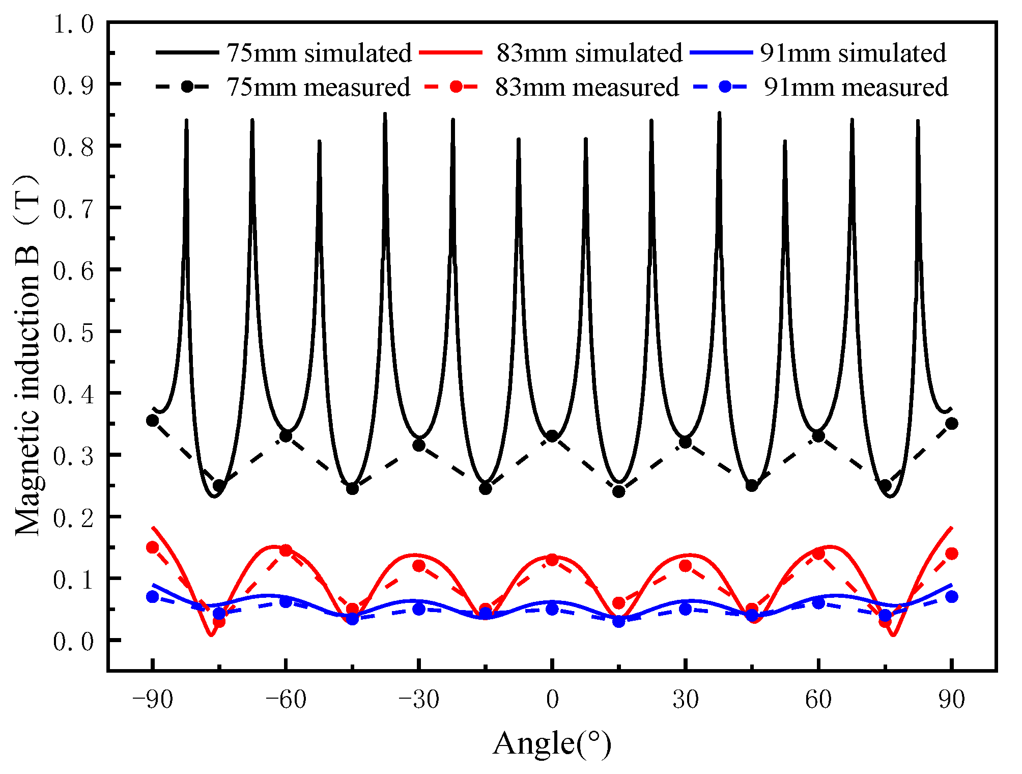
2.2.1. Verification of Magnetic Field
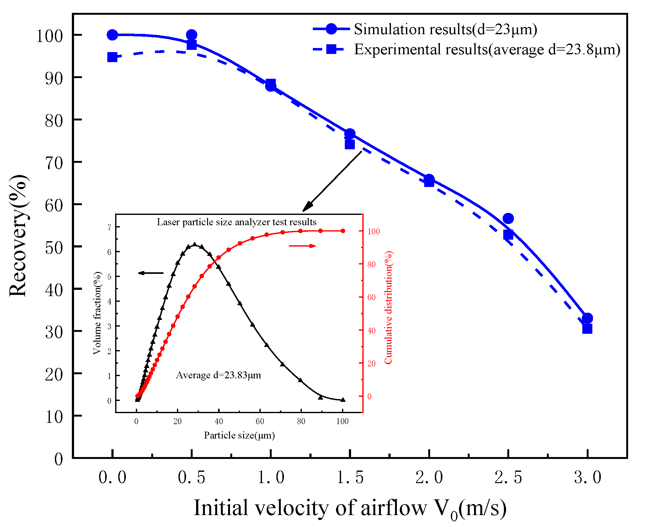
2.2.2. Magnetite Separation Experiment
3. Results and Discussion
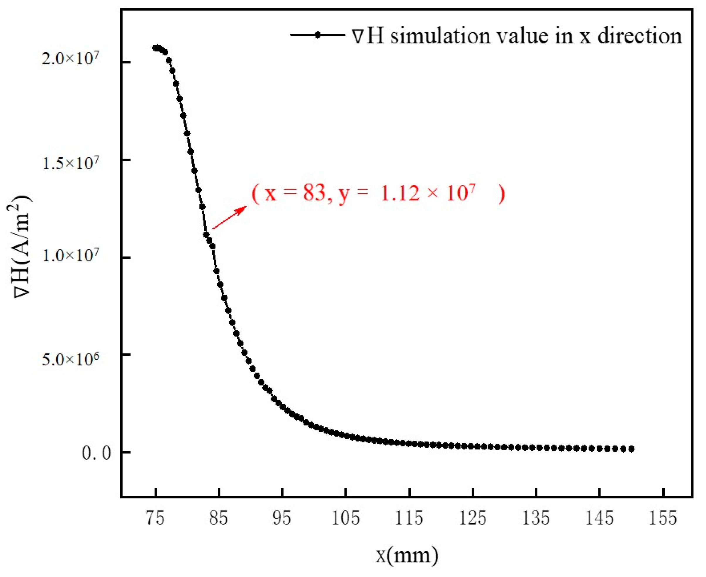
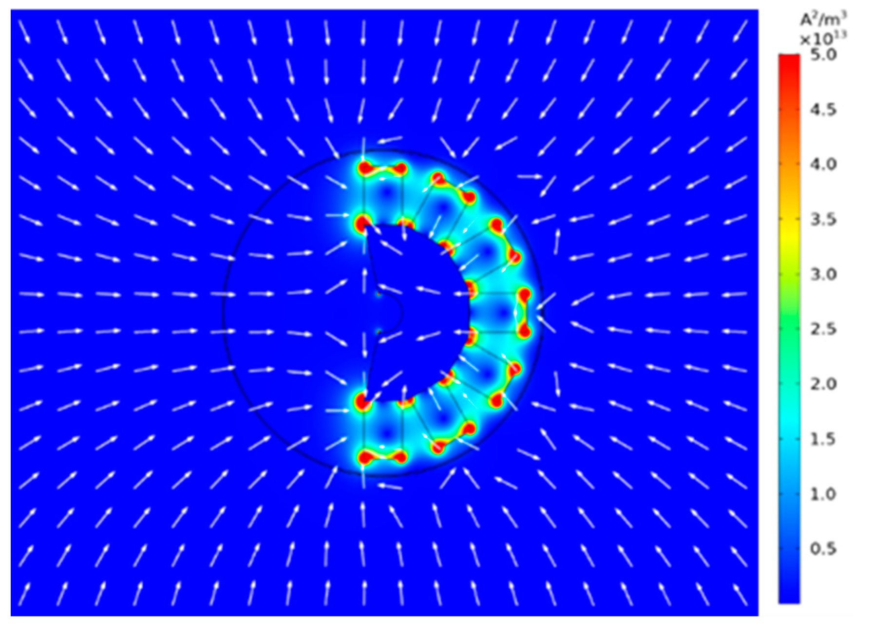
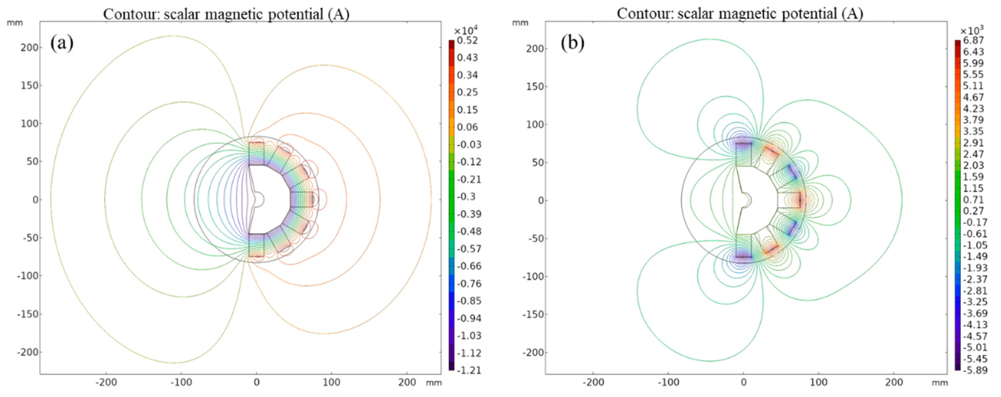
3.1. Magnetic Field Distribution
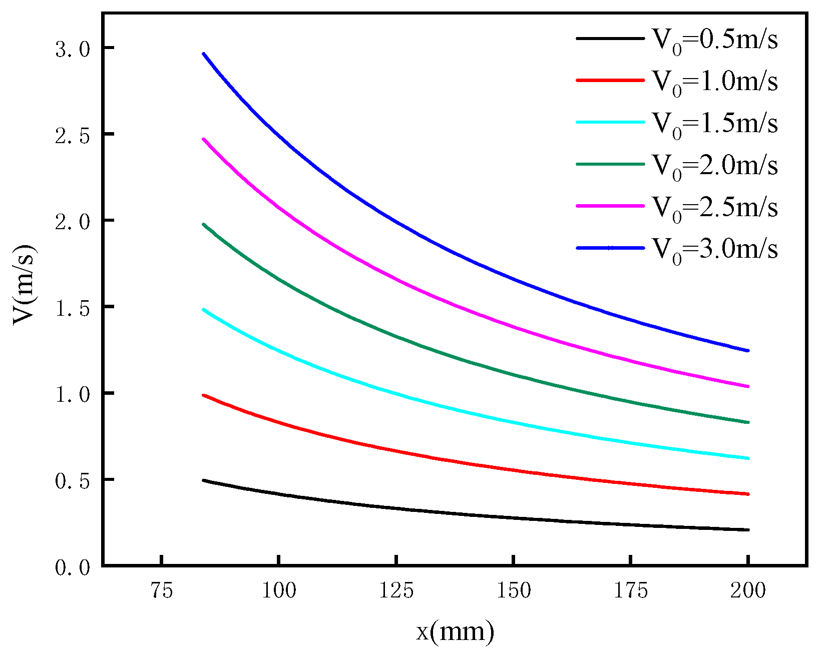
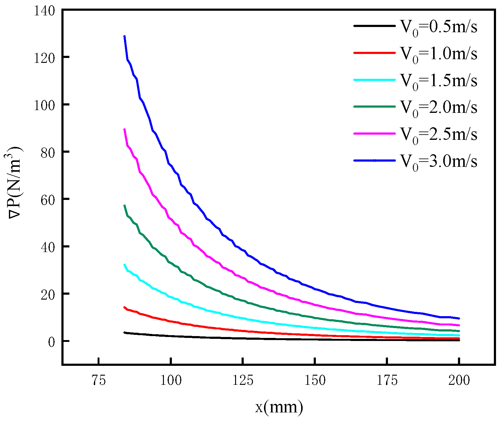
3.2. Flow Field Distribution
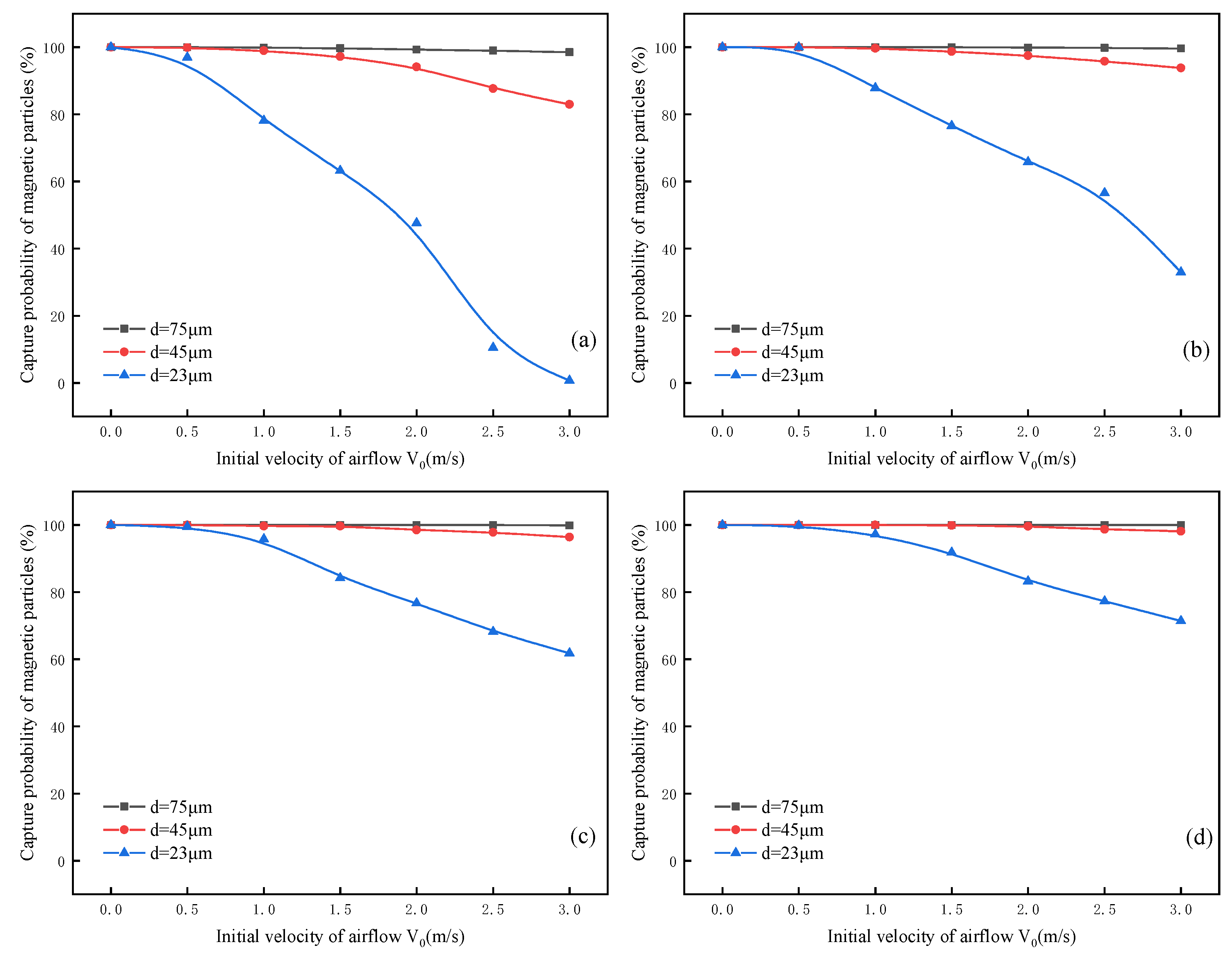
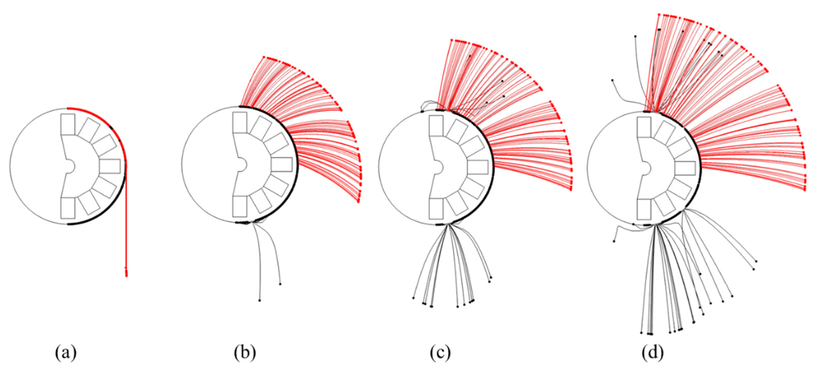
3.3. Particle Motion Behavior
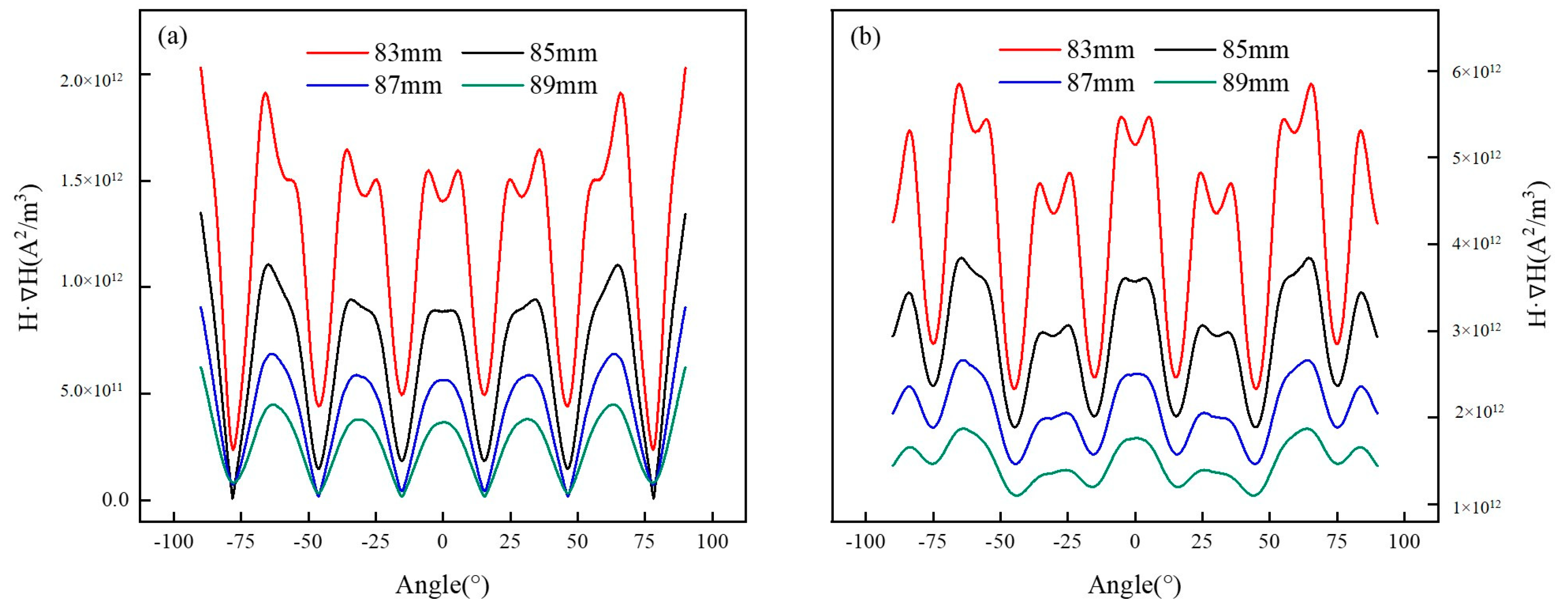
3.4. Optimization Calculation of Magnetic System Structure
4. Conclusions
Supplementary Materials
Author Contributions
Funding
Data Availability Statement
Acknowledgments
Conflicts of Interest
References
- Dworzanowski, M. Optimizing the performance of wet drum magnetic separators. J. S. Afr. Inst. Min. Metall. 2010, 110, 643–653. [Google Scholar]
- Tripathy, S.K.; Banerjee, P.K.; Suresh, N. Separation analysis of dry high intensity induced roll magnetic separator for concentration of hematite fines. Powder Technol. 2014, 264, 527–535. [Google Scholar] [CrossRef]
- Singh, V.; Nag, S.; Tripathy, S.K. Particle flow modeling of dry induced roll magnetic separator. Powder Technol. 2013, 244, 85–92. [Google Scholar] [CrossRef]
- Fu, Y.F.; Yin, W.Z.; Yang, B.; Li, C.; Zhu, Z.L.; Li, D. Effect of sodium alginate on reverse flotation of hematite and its mechanism. Int. J. Miner. Metall. Mater. 2018, 25, 1113–1122. [Google Scholar] [CrossRef]
- Tripathy, S.K.; Banerjee, P.K.; Suresh, N.; Murthy, Y.R.; Singh, V. Dry high-intensity magnetic separation in mineral industry-a review of present status and future prospects. Min Proc. Ext. Metall. Rev. 2017, 38, 339–365. [Google Scholar] [CrossRef]
- Xiong, D.; Lu, L.; Holmes, R.J. Developments in the physical separation of iron ore: Magnetic separation. In Iron Ore; Woodhead Publishing: Southston, UK, 2015; pp. 283–307. [Google Scholar]
- Elder, J.; Sherrell, I. Dry versus wet magnetic separation-horses for courses. In Eight International Heavy Minerals Conference 2011; Curran Associates, Inc.: New York, NY, USA, 2011; pp. 99–106. [Google Scholar]
- Li, Z.J.; Tian, Y.S.; Wang, X.G. Experimental study on cohesion mechanism of mine dust. Min. Saf. Environ. Prot. 2006, 33, 10, 11, 14, 87. [Google Scholar] [CrossRef]
- Ku, J.G.; Liu, X.Y.; Chen, H.H.; Deng, R.D.; Yan, Q.X. Interaction between two magnetic dipoles in a uniform magnetic field. Aip Adv. 2016, 6, 025004. [Google Scholar] [CrossRef]
- Lim, J.K.; Yeap, S.P.; Low, S.C. Challenges associated to magnetic separation of nanomaterials at low field gradient. Sep. Purif. Technol. 2014, 123, 171–174. [Google Scholar] [CrossRef]
- Liu, J.J.; Lu, D.F.; Wang, Y.H.; Zheng, X.Y.; Li, X.D.; Cheng, Z.Y. Effect of dry magnetic separator on pre-selection of magnetite under wind power. Chin. J. Nonferrous Met. 2020, 30, 2482–2491. [Google Scholar]
- Song, S.; Zhang, G.; Luo, Z.; Lv, B. Development of a fluidized dry magnetic separator and its separation performance tests. Miner. Process. Extr. Metall. Rev. 2019, 40, 307–313. [Google Scholar] [CrossRef]
- Mishima, F.; Yamazaki, S.; Yoshida, K.; Nakane, H.; Yoshizawa, S.; Takeda, S. A study on the development of an open-gradient magnetic separator under dry condition. IEEE Trans. Appl. Supercon. 2004, 14, 1561–1564. [Google Scholar] [CrossRef]
- Cheng, K.; Yang, L.L.; Zhang, Z.H. A study on separation iron ore by suspension magnetic separator. Min. Metall. 2008, 17, 20–23. [Google Scholar]
- Wang, S.; Xin, Q. Development and application research of a new type of dry magnetic separator for pulverized ore. Mod. Min 2019, 35, 133–135. [Google Scholar]
- Liu, W.S. Research on air jigging system for dry coal separation. Min. Process. Equip. 2010, 38, 95–98. [Google Scholar]
- Emmanuel, B.; Christopher, K.; Jonas, A.; William, S. Assessing the performance of a novel pneumatic magnetic separator for the beneficiation of magnetite ore. Miner. Eng. 2020, 156, 106483. [Google Scholar]
- Zhang, Z.; Ling, X.; Ma, J. Numerical study on the flow field and separation efficiency of a rotary drum separator. Powder Technol. 2020, 371, 13–25. [Google Scholar] [CrossRef]
- Lu, D.; Liu, J.; Cheng, Z.; Li, X.; Wang, Y. Development of an open-gradient magnetic separator in the aerodynamic field. Physicochem. Probl. Miner. Process. 2020, 56, 325–337. [Google Scholar]
- Geppert, B.; Groeneveld, D.; Loboda, V. Finite-element simulations of a thermoelectric generator and their experimental validation. Acta Crystallogr. 2015, 2, 751–767. [Google Scholar] [CrossRef]
- Huang, H.W.; Wang, J.; Zhao, C.; Mo, Y.L. Two-dimensional finite-element simulation of periodic barriers. J. Eng. Mech. 2021, 147, 04020150. [Google Scholar] [CrossRef]
- Liu, Y.; Cameron, A.T.; Gonzalez, M. Modeling granular material blending in a Tote blender using a finite element method and advection-diffusion Equ. multi-scale model. Powder Technol. 2018, 340, 428–439. [Google Scholar] [CrossRef]
- Lefevre, Y.; Henaux, C.; Llibre, J.F. Magnetic field continuity conditions in finite-element analysis. IEEE Trans. Magn. 2018, 54, 7400304. [Google Scholar] [CrossRef] [Green Version]
- Ouili, M.; Mehasni, R.; Feliachi, M.; Belounis, A.; Latreche, M.E. A simultaneous separation of magnetic and conductive particles in a designed permanent magnet drum separator. Int. J. Appl. Electromagn. Mech. 2019, 61, 137–155. [Google Scholar] [CrossRef]
- Lu, D.; Wang, Y.; He, P.; Sun, W.; Hu, Y. Simulation of magnetic field on tracked permanent magnetic separator based on ANSYS. Chin. J. Nonferrous Met. 2014, 24, 2188–2194. [Google Scholar]
- Zheng, Y.; Li, M.; Cui, R.; Guo, N.; Yan, Y.; Zhang, B. Effect of saturation magnetization of magnetic matrices on performance of high gradient magnetic separator. Met. Mine 2013, 42, 108. [Google Scholar]
- Hu, M.; Wu, B.; Chen, J.; Zeng, J. Numerical simulation of flow field of inflation pressure for large complex sulfide mineral of low-tin flotation machine. Appl. Mech. Mater. 2013, 2516, 333–336. [Google Scholar]
- Wang, X. A Dissertation Submitted in Partial Fulfillment of the Requirements for the Professional Degree of Master in Engineering. Master’s Thesis, Wuhan University of Science and Technology, Wuhan, China, 2017. [Google Scholar]
- Zeng, F.; Wang, Y.; Lu, D.; Li, X.; Zheng, X. Application of self-made reflux classifier in gravity preconcentration of lateritic nickel and flow field simulation thereof. Min. Metall. Eng. 2017, 37, 52–56. [Google Scholar]
- Hu, Y. Analysis on simulation of magnetic separation process using dynamic coupled FEM, CFD and DEM model. Nonferr. Met. Miner. Process. Sect. 2016, 68–72, 82. [Google Scholar] [CrossRef]
- Murariu, V. Simulating a Low Intensity Magnetic Separator Model (LIMS) Using DEM, CFD and FEM Magnetic Design Software. Comput. Modeling 2013. Available online: http://www.researchgate.net/publication/248393907_Simulating_a_Low_Intensity_Magnetic_Separator_Model_LIMS_using_DEM_CFD_and_FEM_Magnetic_Design_Software (accessed on 21 June 2021).
- Karimi, P.; Darban, A.K.; Mansourpour, Z. A finite element model to simulate magnetic field distribution and laboratory studies in wet low-intensity magnetic separator. J. Min. Environ. 2019, 10, 717–727. [Google Scholar]
- Wang, F.; Tang, D.; Gao, L.; Dai, H.; Wang, P.; Gong, Z. Magnetic entrainment mechanism of multi-type intergrowth particles for Low-Intensity magnetic separation based on a multiphysics model. Miner. Eng. 2020, 149, 106264. [Google Scholar] [CrossRef]
- Wang, F.; Dai, H.; Lv, Y.; Zhang, L. Dynamic capture behavior of ferromagnetic particles based on fully coupled multiphysics model of particle-fluid interactions. Miner Eng. 2019, 138, 238–245. [Google Scholar] [CrossRef]
- Xue, Z.; Wang, Y.; Zheng, X.; Lu, D.; Li, X. Particle capture of special cross-section matrices in axial high gradient magnetic separation: A 3D simulation. Sep. Purif. Technol. 2019, 237, 116375. [Google Scholar] [CrossRef]
- Zheng, X.; Wang, Y.; Lu, D. Effect of matrix shape on the capture of fine weakly magnetic minerals in high-gradient magnetic separation. IEEE Trans. Magn. 2016, 52, 7005111. [Google Scholar] [CrossRef]
- Matko, V.; Milanović, M. High Resolution Switching Mode Inductance-to-Frequency Converter with Temperature Compensation. Sensors 2014, 14, 19242–19259. [Google Scholar] [CrossRef] [PubMed]
- Matko, V.; Safarič, R. Major improvements of quartz crystal pulling sensitivity and linearity using series reactance. Sensors 2009, 9, 8263–8270. [Google Scholar] [CrossRef]
- Yang, S.; Tan, M.; Yu, T.; Li, X.; Wang, X.; Zhang, J. Hybrid Reduced Graphene Oxide with Special Magnetoresistance for Wireless Magnetic Field Sensor. Nano-Micro Lett. 2020, 12, 69. [Google Scholar] [CrossRef] [PubMed] [Green Version]
- Avdeev, B.; Dema, R.; Chernyi, S. Study and Modeling of the Magnetic Field Distribution in the Fricker Hydrocyclone Cylindrical Part. Computation 2020, 8, 42. [Google Scholar] [CrossRef]
- Zhang, G. Dynamic Characteristics of Magnetic Separation and Segregation Mechanism of Particles in a Gas-solid Fluidized Magnetic Separator. Ph.D. Thesis, China University of Mining and Technology, Beijing, China, 2019. [Google Scholar]
- Yuan, Z.; Wang, C. Magnetoelectric Mineral Processing, 2nd ed.; Metallurgical Industry Press: Beijing, China, 2015; pp. 12–23. [Google Scholar]


| Parameter | Value | Unit |
|---|---|---|
| Remanence | 1.2 | T |
| Magnetic field intensity on the magnetic surface | 2.63 × 10⁻⁵ | A/m |
| Distance between drum surface and magnetic system surface | 8 × 10⁻³ | m |
| Magnetic pole pitch | 3.93 × 10⁻² | m |
| The radius around which the magnetic poles are arranged | 7.5 × 10⁻² | m |
| Fluid velocity at inlet | 0~3 | m/s |
| Drum velocity | 3; 6; 9; 12 | rad/s |
| Fluid density | 1.29 | |
| Dynamic viscosity of fluid | 1.79 × 10⁻⁵ | Pa·s |
| Particle diameter | 23; 45; 75 | |
| Magnetic particle density/non-magnetic particle density | 5170; 2650 | |
| Relative permeability of magnetic particles | 3.44 | / |
| Vacuum permeability | N/A2 | |
| Acceleration of gravity | 9.8 | |
| Initial temperature | 293.15 | K |
| Initial pressure | 1 | atm |
| 1.0 | 1.2 | 1.4 | 1.6 | |
| Critical velocity (m/s) | 0.95 | 1.35 | 1.77 | 2.27 |
Publisher’s Note: MDPI stays neutral with regard to jurisdictional claims in published maps and institutional affiliations. |
© 2021 by the authors. Licensee MDPI, Basel, Switzerland. This article is an open access article distributed under the terms and conditions of the Creative Commons Attribution (CC BY) license (https://creativecommons.org/licenses/by/4.0/).
Share and Cite
Liu, J.; Xue, Z.; Dong, Z.; Yang, X.; Fu, Y.; Man, X.; Lu, D. Multiphysics Modeling Simulation and Optimization of Aerodynamic Drum Magnetic Separator. Minerals 2021, 11, 680. https://doi.org/10.3390/min11070680
Liu J, Xue Z, Dong Z, Yang X, Fu Y, Man X, Lu D. Multiphysics Modeling Simulation and Optimization of Aerodynamic Drum Magnetic Separator. Minerals. 2021; 11(7):680. https://doi.org/10.3390/min11070680
Chicago/Turabian StyleLiu, Jianjun, Zixing Xue, Zhenhai Dong, Xiaofeng Yang, Yafeng Fu, Xiaofei Man, and Dongfang Lu. 2021. "Multiphysics Modeling Simulation and Optimization of Aerodynamic Drum Magnetic Separator" Minerals 11, no. 7: 680. https://doi.org/10.3390/min11070680
APA StyleLiu, J., Xue, Z., Dong, Z., Yang, X., Fu, Y., Man, X., & Lu, D. (2021). Multiphysics Modeling Simulation and Optimization of Aerodynamic Drum Magnetic Separator. Minerals, 11(7), 680. https://doi.org/10.3390/min11070680