
Integration of Dual Border Effects in Resource Estimation: A Cokriging Practice on a Copper Porphyry Deposit


Abstract
:1. Introduction
2. Methods and Materials
2.1. Resource Modeling
- Converting the geological domain (i.e., categorical data) into indicators at sample locations :
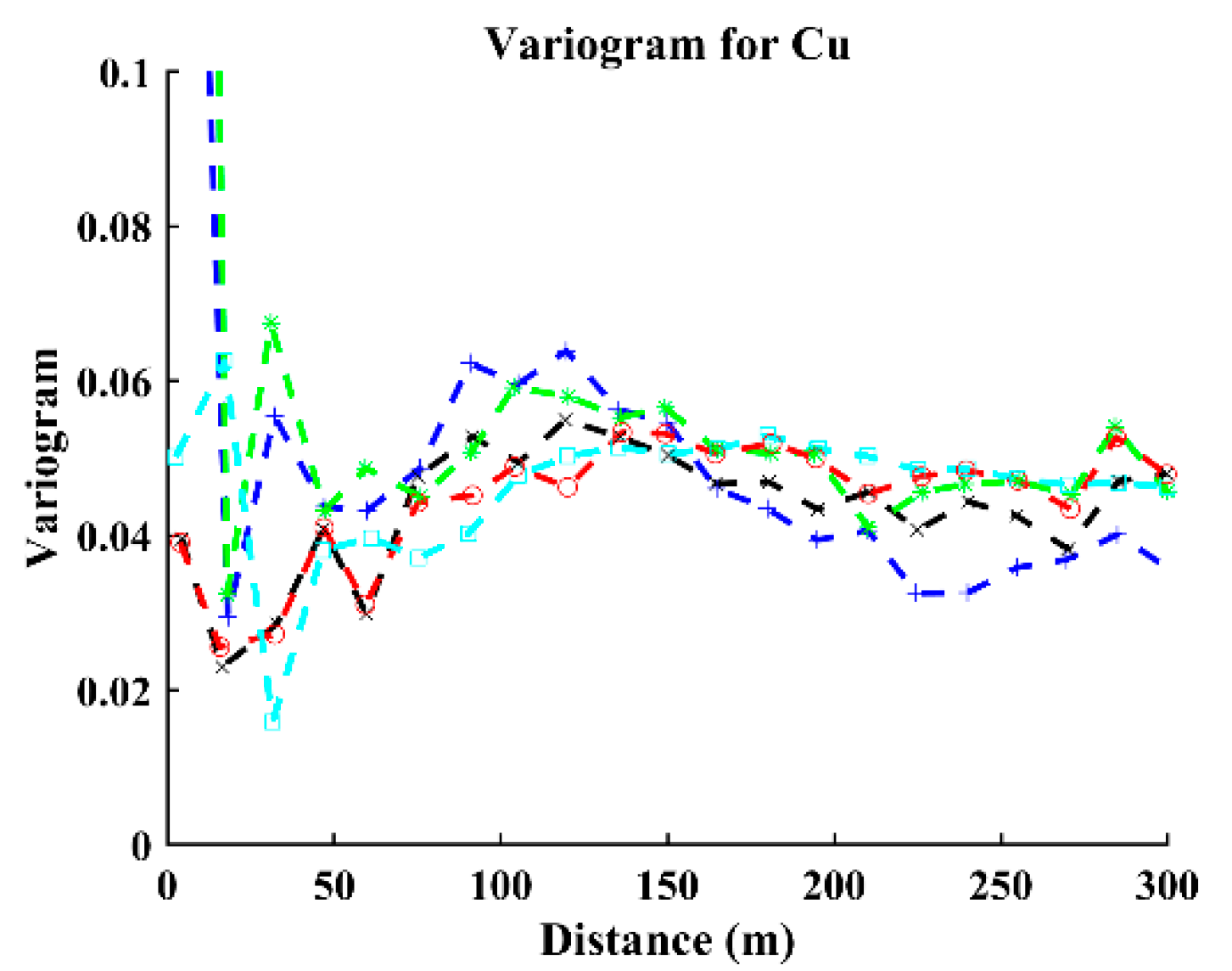
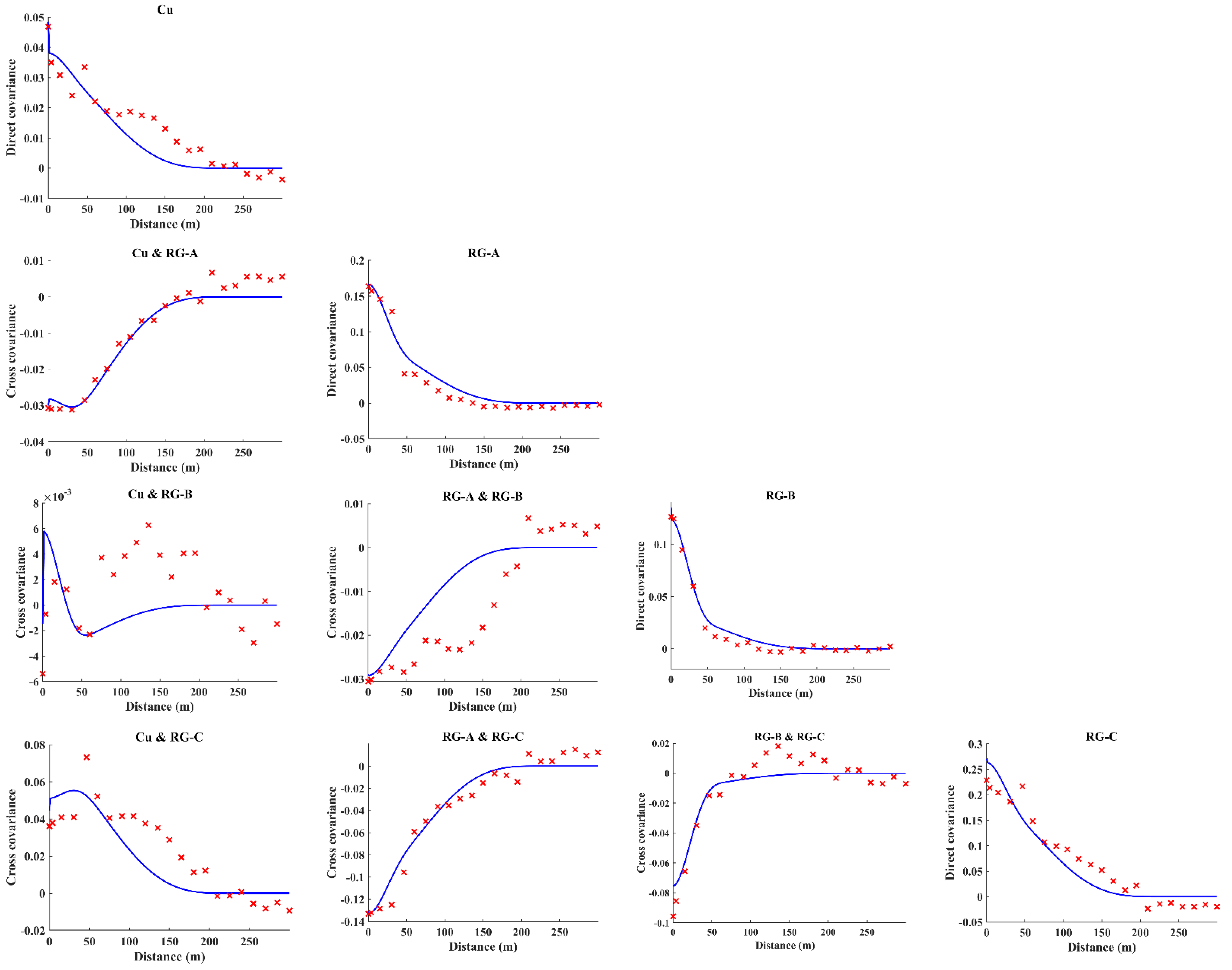
- Computation of experimental direct and cross-variograms or direct and cross-covariances among the continuous variables and indicators. A linear model of coregionalization can be used for fitting purposes [25]. In this step, modeling a coregionalization calls for inferring (n + 1) × (n + 2)/2 direct and cross-variograms or direct and cross-covariances. Assuming numerous indicator variables, a semiautomatic iterative algorithm [26] can be used for fitting purposes.
- Using a cokriging system to estimate the n + 1 variables. The “1” here refers to one continuous variable. If the mean of all n + 1 variables is known, then a simple cokriging is used, and if the mean is unknown, an ordinary cokriging can be considered. The neighborhood can also be moving or unique, depending on the size of conditioning data. The implementation of this cokriging system is provided in the following section.
2.2. The Cokriging System
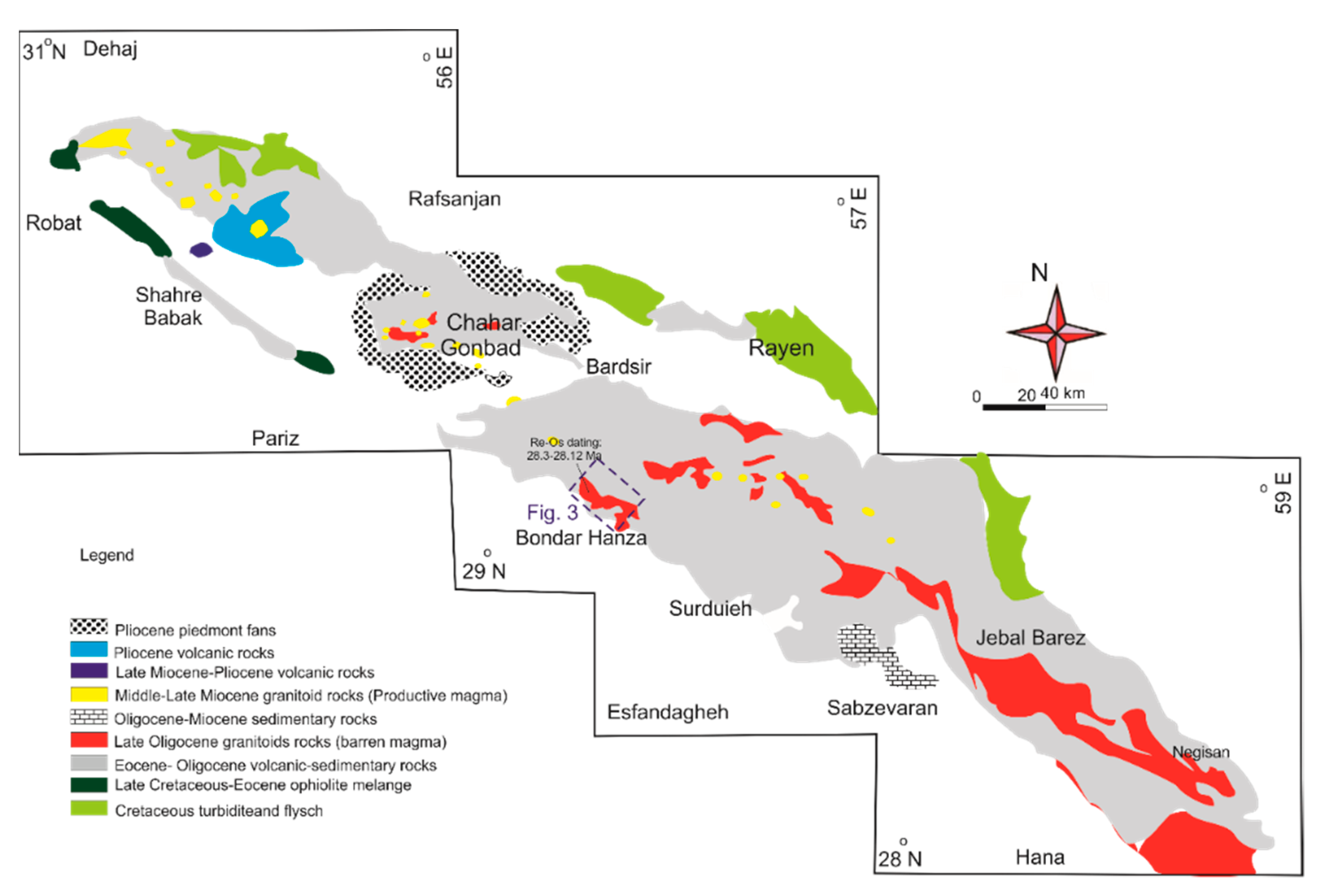
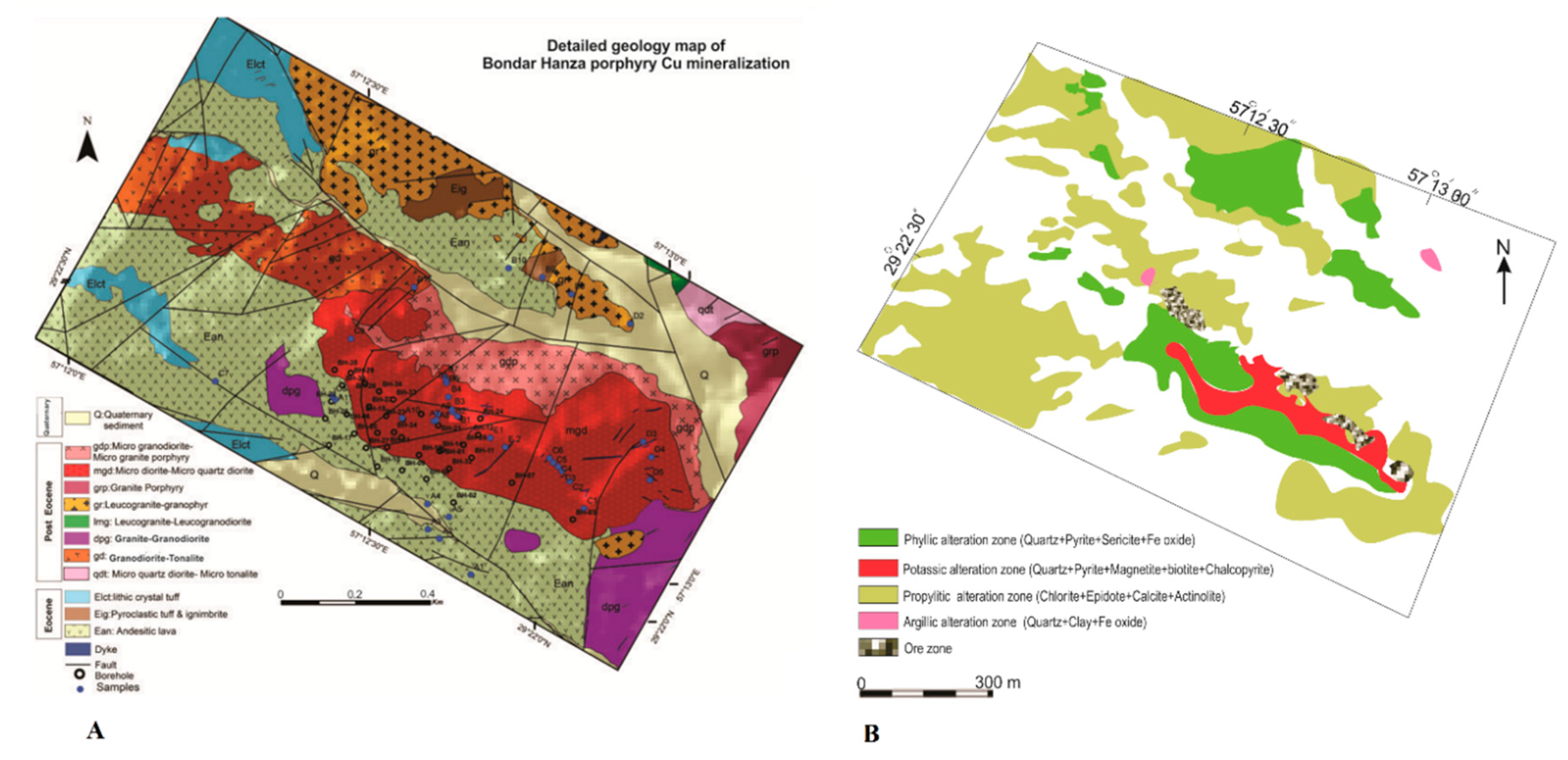
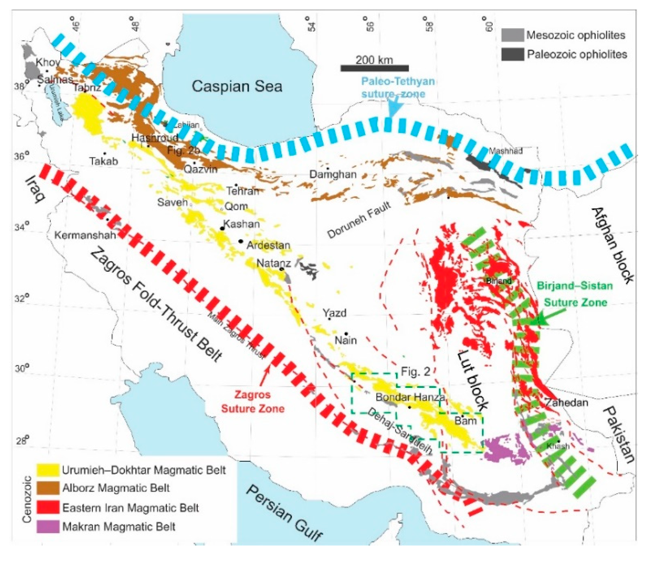
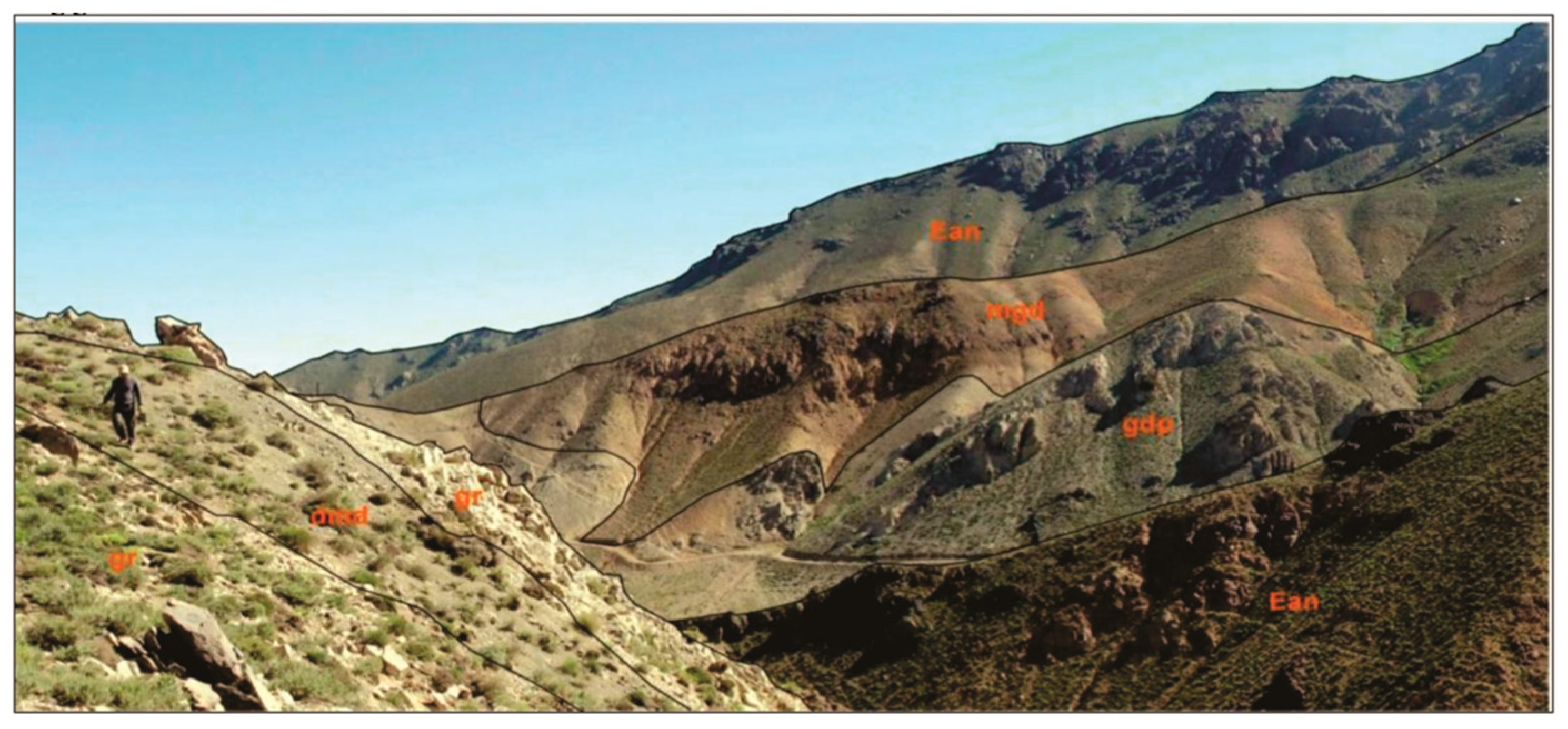
2.3. Geological Setting
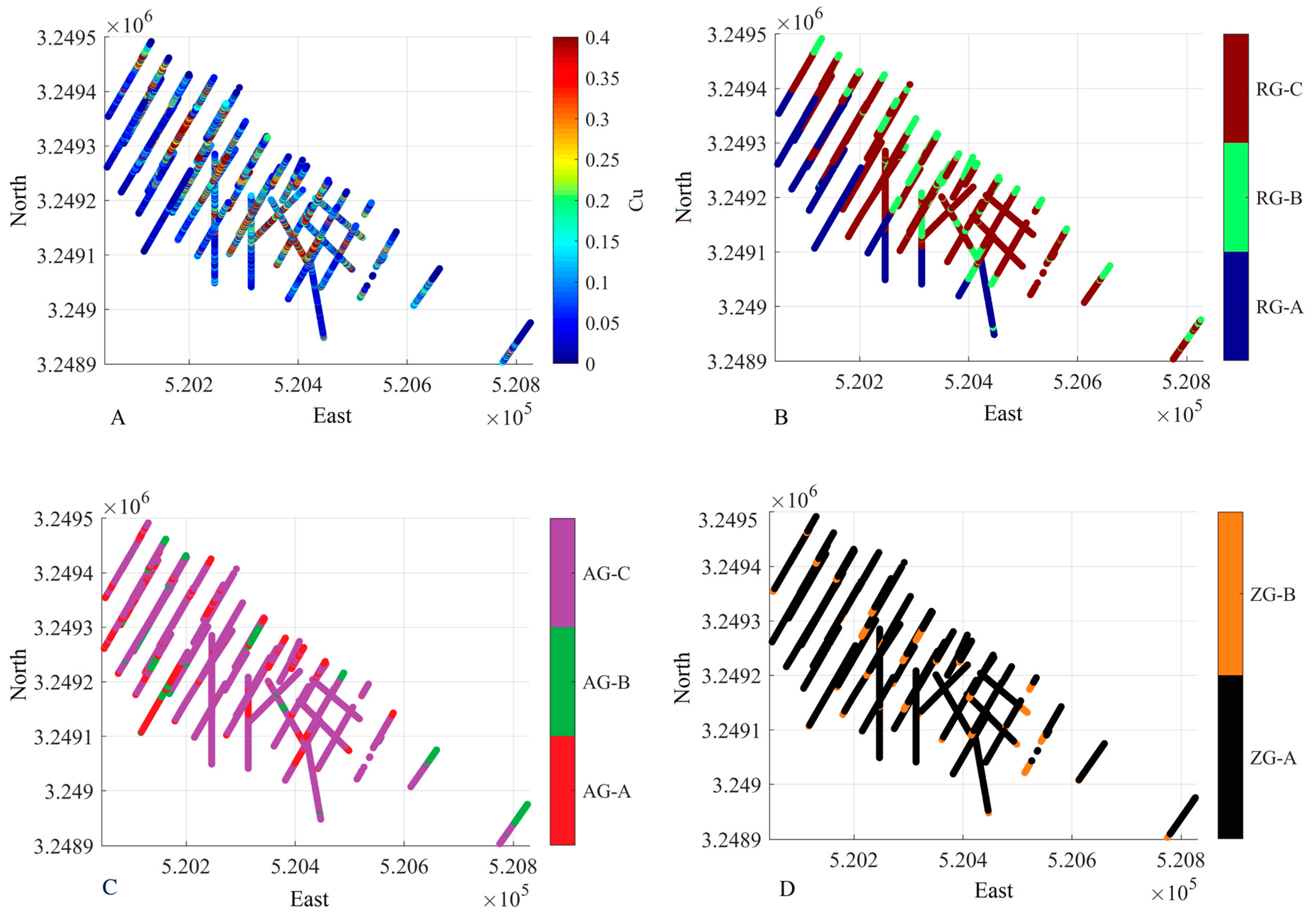
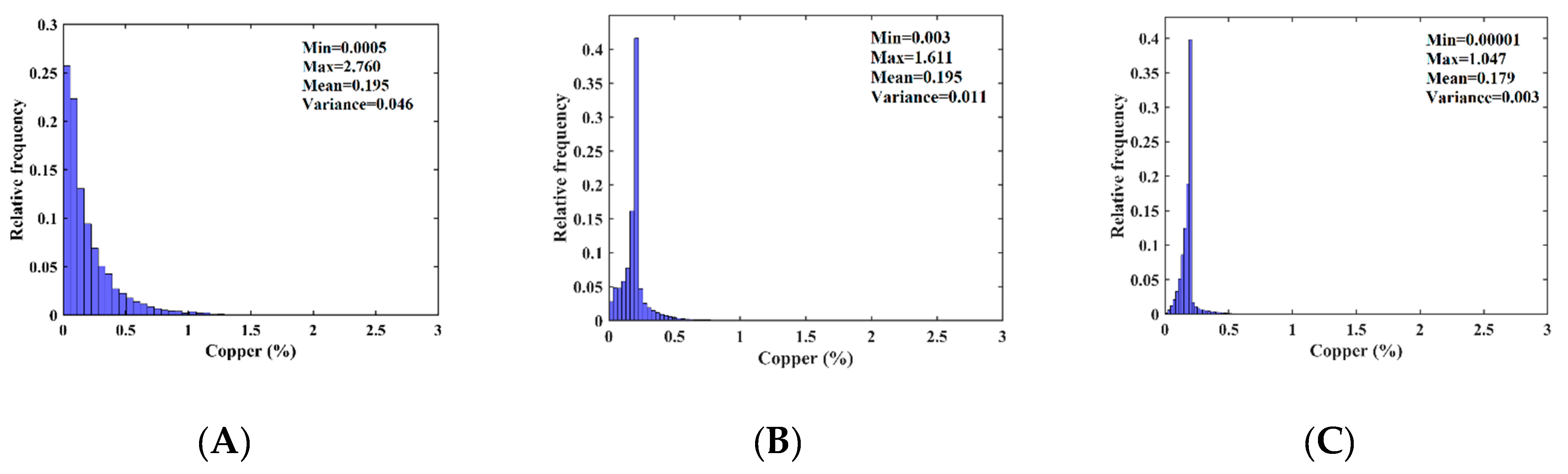
2.4. Presentation of the Dataset
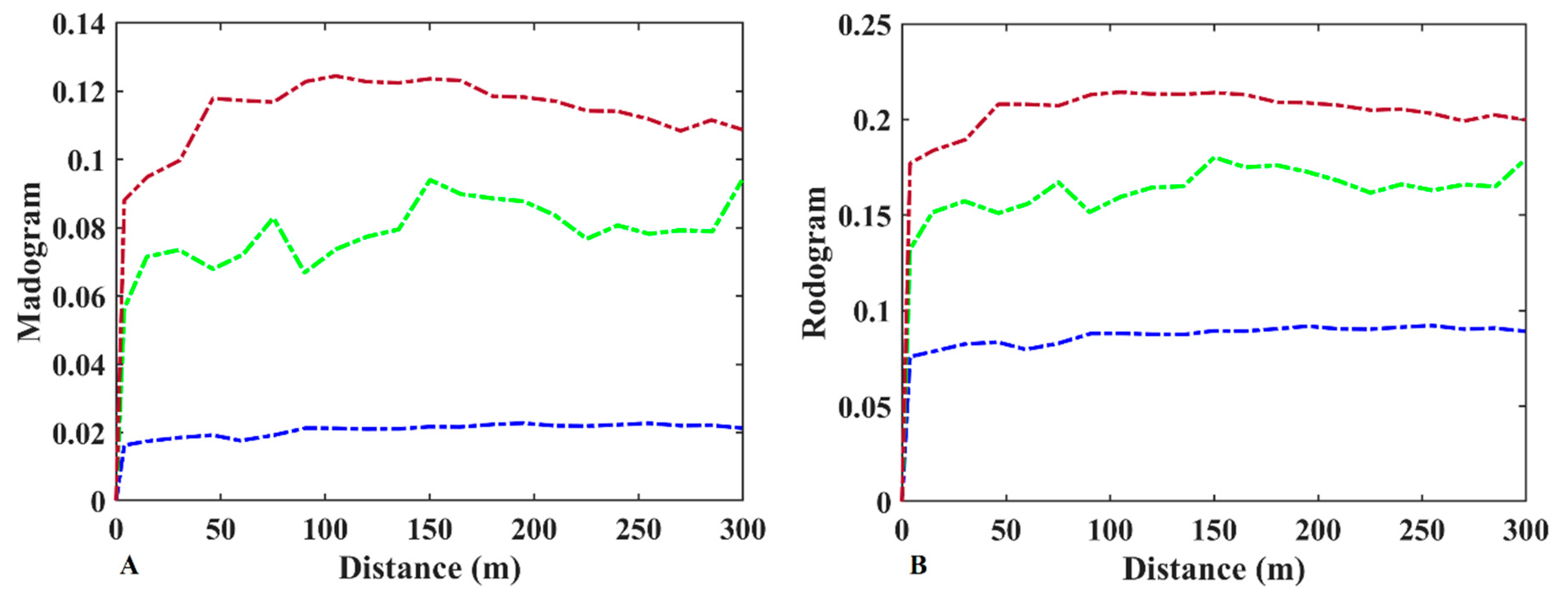
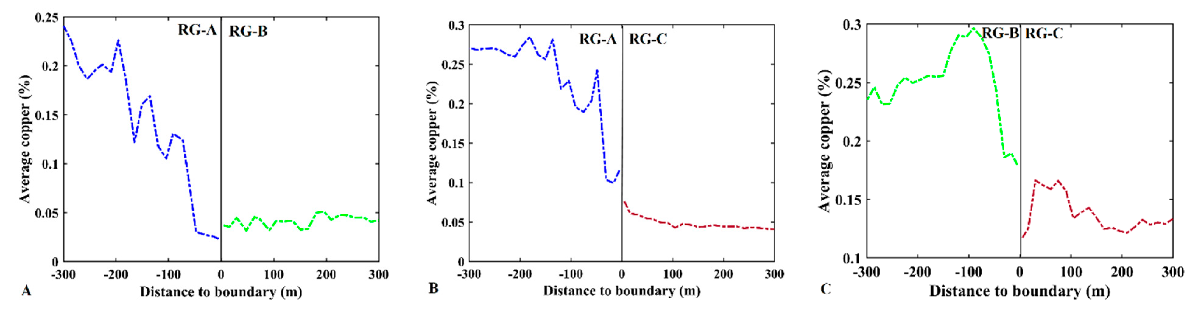
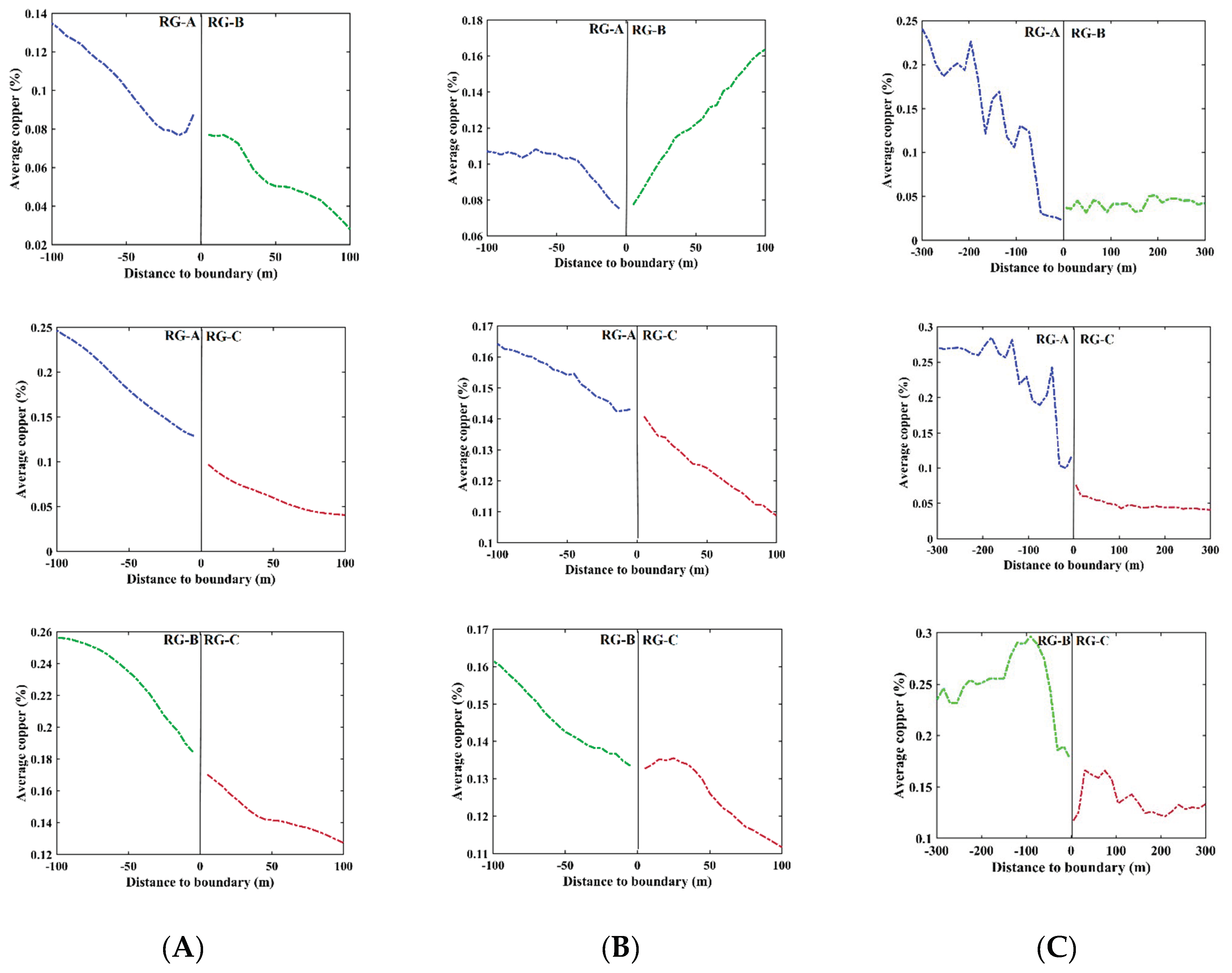
2.5. Contact Analysis
3. Results
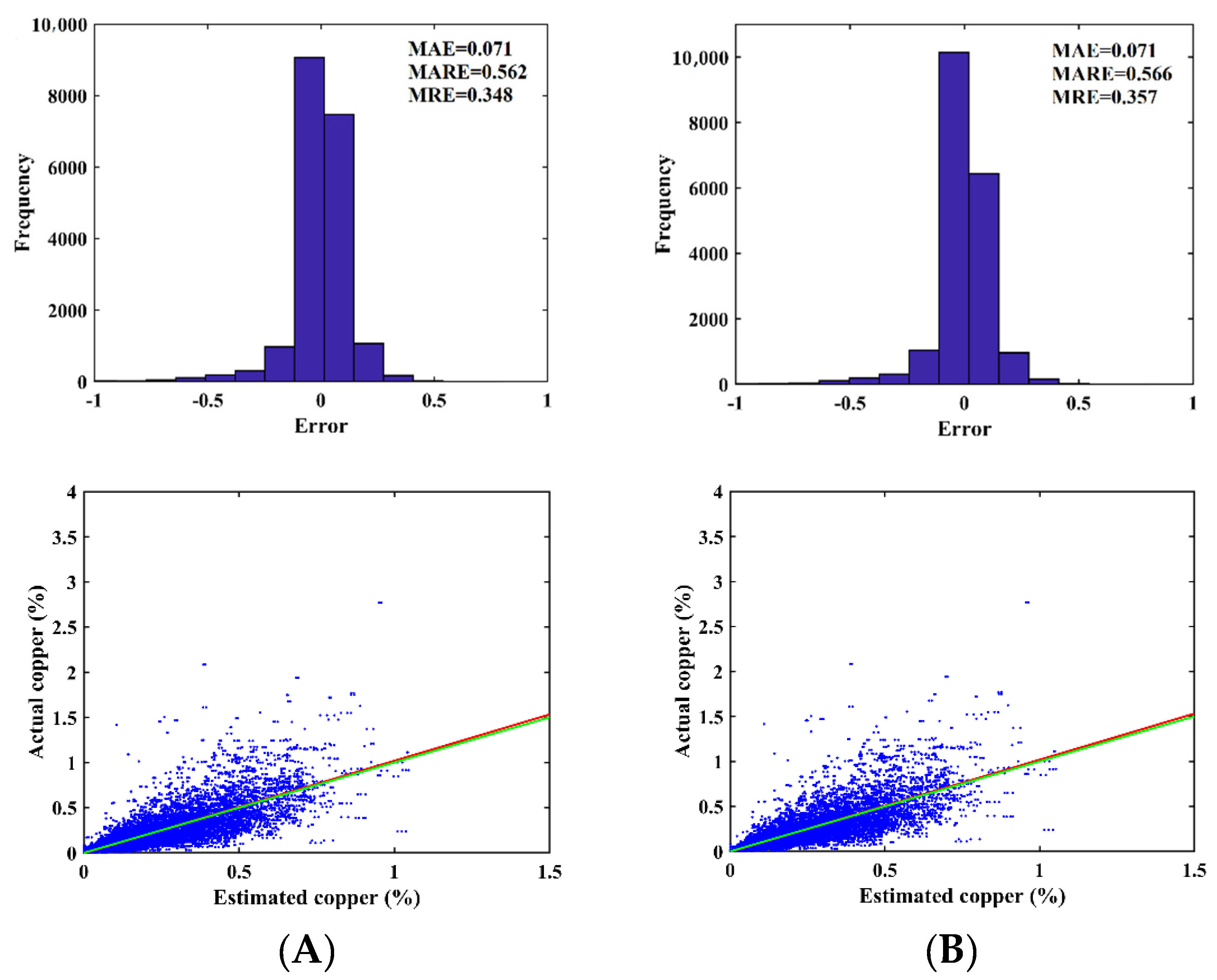
3.1. Validation
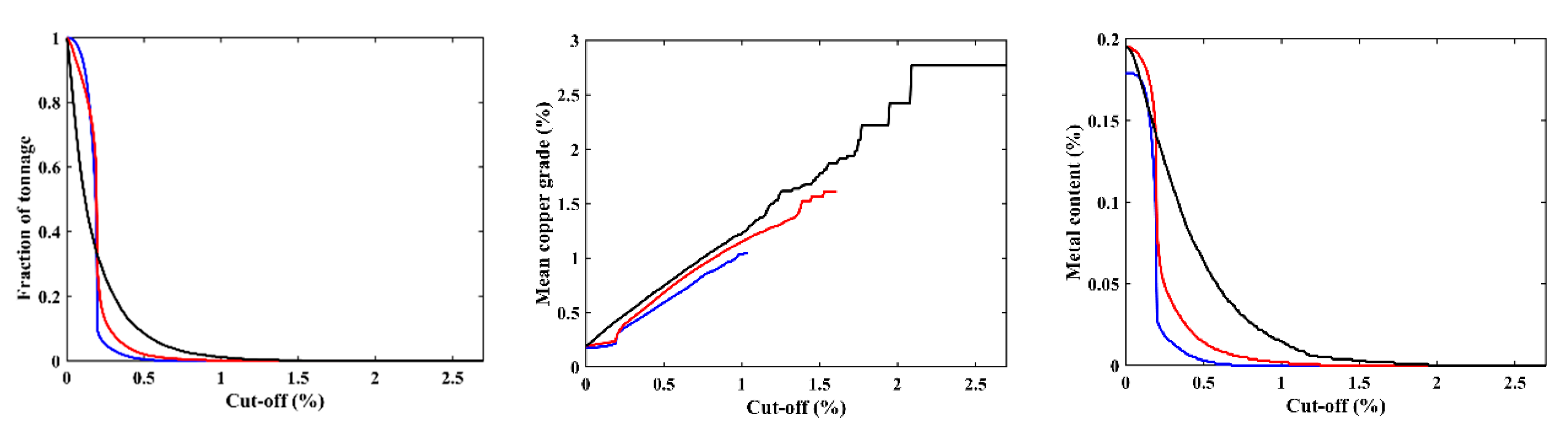
3.2. Recovery Functions
4. Conclusions
Author Contributions
Funding
Data Availability Statement
Acknowledgments
Conflicts of Interest
References
- Sinclair, A.J.; Blackwell, G.H. Applied Mineral Inventory Estimation; Cambridge University Press: Cambridge, UK, 2002. [Google Scholar]
- Emery, X.; Séguret, S.A. Geostatistics for the Mining Industry; CRC Press: Boca Raton, FL, USA, 2020; ISBN 0367505754. [Google Scholar]
- Rossi, M.E.; Deutsch, C.V. Mineral Resource Estimation; Springer: Dordrecht, The Netherlands, 2014; ISBN 9781402057175. [Google Scholar]
- Hustrulid, W.A.; Kuchta, M.; Martin, R.K. (Eds.) Open Pit Mine Planning and Design, Two Volume Set & CD-ROM Pack Hustrulid, 3rd ed.; CRC Press: Boca Raton, FL, USA, 2013; ISBN 1466575123. [Google Scholar]
- Osanloo, M.; Gholamnejad, J.; Karimi, B. Long-term open pit mine production planning: A review of models and algorithms. Int. J. Min. Reclam. Environ. 2008, 22, 3–35. [Google Scholar] [CrossRef]
- Alabert, F.G.; Massonnat, G.J. Heterogeneity in a Complex Turbiditic Reservoir: Stochastic Modelling of Facies and Petrophysical Variability. In Proceedings of the SPE Annual Technical Conference and Exhibition, New Orleans, LA, USA, 23–26 September 1990. [Google Scholar]
- Roldão, D.; Ribeiro, D.; Cunha, E.; Noronha, R.; Madsen, A.; Masetti, L. Combined Use of Lithological and Grade Simulations for Risk Analysis in Iron Ore, Brazil; Springer: Dordrecht, The Netherlands, 2012; pp. 423–434. [Google Scholar]
- Boucher, A.; Dimitrakopoulos, R. Multivariate Block-Support Simulation of the Yandi Iron Ore Deposit, Western Australia. Math. Geosci. 2012, 44, 449–468. [Google Scholar] [CrossRef] [Green Version]
- Jones, P.; Douglas, I.; Jewbali, A. Modeling Combined Geological and Grade Uncertainty: Application of Multiple-Point Simulation at the Apensu Gold Deposit, Ghana. Math. Geosci. 2013, 45, 949–965. [Google Scholar] [CrossRef]
- Carr, J.C.; Beatson, R.K.; Cherrie, J.B.; Mitchell, T.J.; Fright, W.R.; McCallum, B.C.; Evans, T.R. Reconstruction and representation of 3D objects with radial basis functions. In Proceedings of the 28th Annual Conference on Computer Graphics and Interactive Techniques, SIGGRAPH 2001, Los Angeles, CA, USA, 12–17 August 2001; Association for Computing Machinery: New York, NY, USA, 2001; pp. 67–76. [Google Scholar]
- Wang, J.; Zhao, H.; Bi, L.; Wang, L. Implicit 3D modeling of ore body from geological boreholes data using hermite radial basis functions. Minerals 2018, 8, 443. [Google Scholar] [CrossRef] [Green Version]
- Mallet, J.-L. Geomodeling; Oxford University Press: Oxford, UK, 2002. [Google Scholar]
- Mallet, J.L. Discrete Smooth Interpolation. ACM Trans. Graph. 1989, 8, 121–144. [Google Scholar] [CrossRef]
- Houlding, S.W. 3D Geoscience Modeling; Springer: Berlin/Heidelberg, Germany, 1994. [Google Scholar]
- Deutsch, C.V.; Journel, A.G. GSLIB: Geostatistical Software Library and User’s Guide, 2nd ed.; Applied Geostatistics Series; Oxford University Press: Oxford, UK, 1998; ISBN 0195100158. [Google Scholar]
- Krige, D.G. A practical analysis of the effects of spatial structure and of data available and accessed, on conditional biases in ordinary kriging. In Proceedings of the International Geostatistics Congress, Wollongong, Australia, 22–27 September 1996; Baafi, E., Schofield, N., Eds.; Kluwer Academic: Dordrecht, The Netherlands, 1996; pp. 799–810. [Google Scholar]
- Pereira, P.E.C.; Rabelo, M.N.; Ribeiro, C.C.; Diniz-Pinto, H.S. Geological modeling by an indicator kriging approach applied to a limestone deposit in indiara city-goiás. Rev. Esc. Minas 2017, 70, 331–337. [Google Scholar] [CrossRef] [Green Version]
- Wilde, B.J.; Deutsch, C.V. Kriging and Simulation in Presence of Stationary Domains: Developments in Boundary Modeling. In Geostatistics Oslo 2012; Quantitative Geology and Geostatistics; Abrahamsen, P., Hauge, R., Kolbjørnsen, O., Eds.; Springer: Berlin/Heidelberg, Germany, 2012; pp. 289–300. [Google Scholar]
- Larrondo, P.; Deutsch, C. V Methodology for Geostatistical Model of Gradational Geological Boundaries: Local Non-stationary LMC. Cent. Comput. Geostat. 2004, 6, 1–17. [Google Scholar]
- Emery, X.; Ortiz, J. Geostatistical estimation of mineral resources with soft geological boundaries: A comparative study. J. S. Afr. Inst. Min. Metall. 2006, 106, 577–584. [Google Scholar]
- Emery, X.; Ortiz, J. Estimation of mineral resources using grade domains: Critical analysis and a suggested methodology. J. S. Afr. Inst. Min. Metall. 2005, 105, 247–255. [Google Scholar]
- Séguret, S.A. Analysis and Estimation of Multi-unit Deposits: Application to a Porphyry Copper Deposit. Math. Geosci. 2013, 45, 927–947. [Google Scholar] [CrossRef] [Green Version]
- Kasmaee, S.; Raspa, G.; de Fouquet, C.; Tinti, F.; Bonduà, S.; Bruno, R. Geostatistical Estimation of Multi-Domain Deposits with Transitional Boundaries: A Sensitivity Study for the Sechahun Iron Mine. Minerals 2019, 9, 115. [Google Scholar] [CrossRef] [Green Version]
- Adeli, A.; Emery, X. Geostatistical simulation of rock physical and geochemical properties with spatial filtering and its application to predictive geological mapping. J. Geochem. Explor. 2021, 220, 106661. [Google Scholar] [CrossRef]
- Goovaerts, P. Geostatistics for Natural Resources Evaluation; Oxford University Press: Oxford, UK, 1997; ISBN 0195115384. [Google Scholar]
- Emery, X. Iterative algorithms for fitting a linear model of coregionalization. Comput. Geosci. 2010, 36, 1150–1160. [Google Scholar] [CrossRef]
- Goovaerts, P. Geostatistical modelling of uncertainty in soil science. Geoderma 2001, 103, 3–26. [Google Scholar] [CrossRef]
- Sepidbar, F.; Shafaii Moghadam, H.; Zhang, L.; Li, J.W.; Ma, J.; Stern, R.J.; Lin, C. Across-arc geochemical variations in the Paleogene magmatic belt of Iran. Lithos 2019, 344–345, 280–296. [Google Scholar] [CrossRef]
- Sepidbar, F.; Mirnejad, H.; Ma, C.; Moghadam, H.S. Identification of Eocene-Oligocene magmatic pulses associated with flare-up in east Iran: Timing and sources. Gondwana Res. 2018, 57, 141–156. [Google Scholar] [CrossRef]
- Shafaii Moghadam, H.; Li, Q.L.; Li, X.H.; Stern, R.J.; Levresse, G.; Santos, J.F.; Lopez Martinez, M.; Ducea, M.N.; Ghorbani, G.; Hassannezhad, A. Neotethyan Subduction Ignited the Iran Arc and Backarc Differently. J. Geophys. Res. Solid Earth 2020, 125, e2019JB018460. [Google Scholar] [CrossRef]
- Verdel, C.; Wernicke, B.P.; Hassanzadeh, J.; Guest, B. A Paleogene extensional arc flare-up in Iran. Tectonics 2011, 30, 3008. [Google Scholar] [CrossRef] [Green Version]
- Topuz, G.; Altherr, R.; Schwarz, W.H.; Siebel, W.; Satır, M.; Dokuz, A. Post-collisional plutonism with adakite-like signatures: The Eocene Saraycik granodiorite (Eastern Pontides, Turkey). Contrib. Mineral. Petrol. 2005, 150, 441–455. [Google Scholar] [CrossRef]
- Pang, K.N.; Chung, S.L.; Zarrinkoub, M.H.; Khatib, M.M.; Mohammadi, S.S.; Chiu, H.Y.; Chu, C.H.; Lee, H.Y.; Lo, C.H. Eocene-Oligocene post-collisional magmatism in the Lut-Sistan region, eastern Iran: Magma genesis and tectonic implications. Lithos 2013, 180–181, 234–251. [Google Scholar] [CrossRef]
- Berberian, M.; King, G.C.P. Towards a paleogeography and tectonic evolution of Iran. Can. J. Earth Sci. 1981, 18, 210–265. [Google Scholar] [CrossRef]
- Haschke, M.; Ahmadian, J.; Murata, M.; Mcdonald, I. Copper mineralization prevented by Arc-root delamination during Alpine-Himalayan collision in central Iran. Econ. Geol. 2010, 105, 855–865. [Google Scholar] [CrossRef]
- Asadi, S.; Moore, F.; Zarasvandi, A. Discriminating productive and barren porphyry copper deposits in the southeastern part of the central Iranian volcano-plutonic belt, Kerman region, Iran: A review. Earth-Sci. Rev. 2014, 138, 25–46. [Google Scholar] [CrossRef]
- Sepidbar, F.; Ao, S.; Palin, R.M.; Li, Q.L.; Zhang, Z. Origin, age and petrogenesis of barren (low-grade) granitoids from the Bezenjan-Bardsir magmatic complex, southeast of the Urumieh-Dokhtar magmatic belt, Iran. Ore Geol. Rev. 2019, 104, 132–147. [Google Scholar] [CrossRef]
- Mohebi, A.; Mirnejad, H.; Lentz, D.; Behzadi, M.; Dolati, A.; Kani, A.; Taghizadeh, H. Controls on porphyry Cu mineralization around Hanza Mountain, south-east of Iran: An analysis of structural evolution from remote sensing, geophysical, geochemical and geological data. Ore Geol. Rev. 2015, 69, 187–198. [Google Scholar] [CrossRef]
- Mohebi, A.; Sepidbar, F.; Mirnejad, H.; Behzadi, M. Molybdenite Re–Os dating, petrology, and geochemistry of granitoids in the Bondar Hanza porphyry Cu deposit (Urumieh-Dokhtar magmatic arc), Iran: Insight into petrogenesis, mineralization, and tectonic setting. Geol. J. 2020, 55, 7499–7516. [Google Scholar] [CrossRef]
- Shafiei, B.; Shahabpour, J. Gold Distribution in Porphyry Copper Deposits of Kerman Region, Southeastern Iran. J. Sci. Islam. Repub. Iran 2008, 19, 247–260. [Google Scholar]
- Shafiei, B.; Haschke, M.; Shahabpour, J. Recycling of orogenic arc crust triggers porphyry Cu mineralization in Kerman Cenozoic arc rocks, southeastern Iran. Miner. Depos. 2009, 44, 265–283. [Google Scholar] [CrossRef]
- Boomeri, M.; Nakashima, K.; Lentz, D.R. The Miduk porphyry Cu deposit, Kerman, Iran: A geochemical analysis of the potassic zone including halogen element systematics related to Cu mineralization processes. J. Geochem. Explor. 2009, 103, 17–29. [Google Scholar] [CrossRef]
- Boomeri, M.; Nakashima, K.; Lentz, D.R. The Sarcheshmeh porphyry copper deposit, Kerman, Iran: A mineralogical analysis of the igneous rocks and alteration zones including halogen element systematics related to Cu mineralization processes. Ore Geol. Rev. 2010, 38, 367–381. [Google Scholar] [CrossRef]
- Hezarkhani, A. Withdrawn: Mass changes during hydrothermal alteration/mineralization in a porphyry copper deposit, eastern Sungun, northwestern Iran. J. Asian Earth Sci. 2003. [Google Scholar] [CrossRef]
- Maleki, M.; Emery, X. Joint Simulation of Grade and Rock Type in a Stratabound Copper Deposit. Math. Geosci. 2015, 47, 471–495. [Google Scholar] [CrossRef]
- Maleki, M.; Madani, N.; Emery, X. Capping and kriging grades with long-tailed distributions. J. S. Afr. Inst. Min. Metall. 2014, 114, 255–263. [Google Scholar]
- Madani, N. Application of projection pursuit multivariate transform to alleviate the smoothing effect in cokriging approach for spatial estimation of cross-correlated variables. Boll. Geofis. Teor. Appl. 2019, 60, 583–598. [Google Scholar] [CrossRef]
- Walvoort, D.J.J.; De Gruijter, J.J. Compositional kriging: A spatial interpolation method for compositional data. Math. Geol. 2001, 33, 951–966. [Google Scholar] [CrossRef]
- Wackernagel, H. Multivariate Geostatistics: An Introduction with Applications; Springer: Berlin/Heidelberg, Germany, 2013. [Google Scholar]


| Alteration | Group A | ARG-PHY |
| Group B | PRP-SLC | |
| Group C | POT | |
| Rock type | Group A | AND-IGB-LTT-TUF |
| Group B | QDI- GRD | |
| Group C | MTV | |
| Zone | Group A | HYP |
| Group B | LEA-OXI-(OXI-HYP)-(OXI-SUP)-SUP-(SUP-HYP) |
| Continuous Variable | Mean | Variance | Median | COV |
|---|---|---|---|---|
| Cu (%) | 0.195 | 0.046 | 0.120 | 1.107 |
| Categorical variable | Proportion | |||
| Alternation group-A | 0.123 | |||
| Alternation group-B | 0.053 | |||
| Alternation group C | 0.823 | |||
| Rock group-A | 0.206 | |||
| Rock group-B | 0.146 | |||
| Rock group-C | 0.645 | |||
| Zone group-A | 0.926 | |||
| Zone group-B | 0.073 | |||
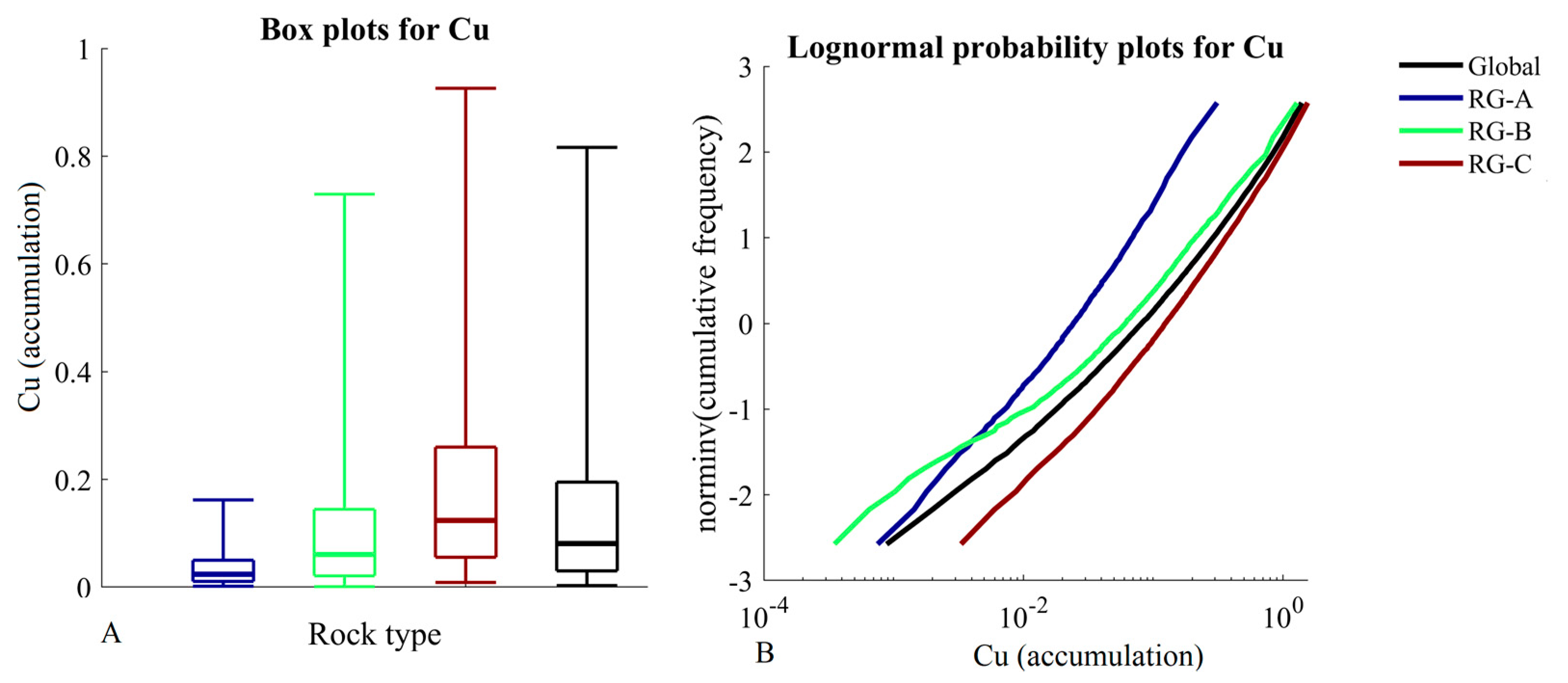
| Statistical Parameter | RG-A | RG-B | RG-C |
|---|---|---|---|
| Minimum | 0.00/0.00/0.00 | 0.00/0.00/0.00 | 0.00/0.00/0.00 |
| Maximum | 0.82/0.99/1.01 | 1.72/0.20/0.65 | 2.76/0.59/0.63 |
| Mean | 0.04/0.15/0.16 | 0.15/0.02/0.12 | 0.25/0.10/0.10 |
| Variance | 0.003/0.003/0.002 | 0.04/0.001/0.002 | 0.05/0.007/0.007 |
| Title | Case I | Case II |
|---|---|---|
| Accuracy | 0.992 | 0.955 |
| Precision for RG-A | 0.997 | 0.905 |
| Precision for RG-B | 0.985 | 0.933 |
| Precision for RG-C | 0.992 | 0.976 |
Publisher’s Note: MDPI stays neutral with regard to jurisdictional claims in published maps and institutional affiliations. |
© 2021 by the authors. Licensee MDPI, Basel, Switzerland. This article is an open access article distributed under the terms and conditions of the Creative Commons Attribution (CC BY) license (https://creativecommons.org/licenses/by/4.0/).
Share and Cite
Madani, N.; Maleki, M.; Sepidbar, F. Integration of Dual Border Effects in Resource Estimation: A Cokriging Practice on a Copper Porphyry Deposit. Minerals 2021, 11, 660. https://doi.org/10.3390/min11070660
Madani N, Maleki M, Sepidbar F. Integration of Dual Border Effects in Resource Estimation: A Cokriging Practice on a Copper Porphyry Deposit. Minerals. 2021; 11(7):660. https://doi.org/10.3390/min11070660
Chicago/Turabian StyleMadani, Nasser, Mohammad Maleki, and Fatemeh Sepidbar. 2021. "Integration of Dual Border Effects in Resource Estimation: A Cokriging Practice on a Copper Porphyry Deposit" Minerals 11, no. 7: 660. https://doi.org/10.3390/min11070660
APA StyleMadani, N., Maleki, M., & Sepidbar, F. (2021). Integration of Dual Border Effects in Resource Estimation: A Cokriging Practice on a Copper Porphyry Deposit. Minerals, 11(7), 660. https://doi.org/10.3390/min11070660