Article

Spectral Tomography for 3D Element Detection and Mineral Analysis

by
Jose R. A. Godinho
1,*,
Gabriel Westaway-Heaven
1,
Marijn A. Boone
2 and
Axel D. Renno
1
1
Helmholtz Institute Freiberg for Resource Technology, Helmholtz-Zentrum Dresden-Rossendorf, Chemnitzer Straße 40, 09599 Freiberg, Germany
2
TESCAN XRE, Bollebergen 2B Box 1, 9052 Ghent, Belgium
*
Author to whom correspondence should be addressed.
Minerals 2021, 11(6), 598; https://doi.org/10.3390/min11060598
Submission received: 8 April 2021 / Revised: 21 May 2021 / Accepted: 25 May 2021 / Published: 1 June 2021

Abstract

:
This paper demonstrates the potential of a new 3D imaging technique, Spectral Computed Tomography (sp-CT), to identify heavy elements inside materials, which can be used to classify mineral phases. The method combines the total X-ray transmission measured by a normal polychromatic X-ray detector, and the transmitted X-ray energy spectrum measured by a detector that discriminates between X-rays with energies of about 1.1 keV resolution. An analysis of the energy spectrum allows to identify sudden changes of transmission at K-edge energies that are specific of each element. The additional information about the elements in a phase improves the classification of mineral phases from grey-scale 3D images that would be otherwise difficult due to artefacts or the lack of contrast between phases. The ability to identify the elements inside the minerals that compose ore particles and rocks is crucial to broaden the application of 3D imaging in Earth sciences research and mineral process engineering, which will represent an important complement to traditional 2D imaging mineral characterization methods. In this paper, the first applications of sp-CT to classify mineral phases are showcased and the limitations and further developments are discussed.

Graphical Abstract

1. Introduction

Benchtop X-ray computed micro-tomography (CT) is the prime technique for non-invasive 3D imaging used across the different fields of research and industry [1,2]. Using CT, the 3D microstructure of a sample can be represented by voxelized images where the intensity of a voxel (grey-scale value) is a function of the electron density of the elements in the microstructure. Thereafter, phases with similar grey-scale values, e.g., minerals and mineral aggregates, may be segmented for individual analyses and quantification [3]. From this analysis, 3D parameters, such as volumes, grain sizes and surface areas can be measured, and also the spatial distribution and associations of individual particles or phases can be determined [4,5,6,7,8,9]. Other advantages of CT include the minimum requirements of sample preparation and its non-destructive nature permit time-lapse and in situ studies where changes in a sample’s microstructure during a process can be imaged [10].
Despite the many advantages of CT, interpreting 3D grey-scale images can be challenging, especially for complex polyphase samples. For example, classifying a voxel as a specific phase based only on the voxel intensity may not be possible since minerals with different chemical compositions can have similar electron densities, i.e., a similar X-ray attenuation coefficient [11]. Therefore, direct classification of a phase, similar to how it is done with 2D surface imaging techniques that use chemical information, such as mineral liberation analysis, MLA [12] and Hyperspectral [13], is not possible. Additionally, imaging artefacts and partial volume effects broadens the intensity range attributed to a phase [7,14]; thus, frequently causing an overlap between the ranges of grey-scale that could be attributed to different phases.
Many of these challenges arise from the polychromatic nature of X-rays emitted by commercial scanners for which the intensity of X-rays with some energy depends on the scanner acquisition parameters chosen by the operator [15]. Additionally, the amount X-rays become attenuated by a material depends on the X-ray energy and on the sample thickness and overall density. Therefore, it is difficult to predict the energy spectrum transmitted through samples with complex matrixes. Nevertheless, normal X-ray detectors only measure the total amount of X-rays (all energies) hitting a pixel. That means, the energy-specific attenuation spectrum of the sample that carries the chemical information is lost at the detector [14]. Alternative methods can be used to retrieve chemical information into the final grey-scale of the 3D image [16]. For example, using monochromatic synchrotron X-rays, dual or multi energy scanning [17,18,19], or the use of photon counting detectors that can resolve the energy of single photons [20,21,22]. Nevertheless, it is difficult to obtain time at synchrotrons, dual energy scanning requires preliminary knowledge about the element of interest and requires a time-consuming optimization for each new material, and photon counting detectors are less efficient, thus requiring scanning times often longer than a day. In summary, there is no practical solution to obtain direct chemical information in 3D images obtained from CT.
Here, we propose a new method that adds elemental information to 3D images, by combining information from a traditional X-ray detector (detects the total number of counts in a pixel) with an energy selective line detector (detects the number of counts of X-rays with specific energies). Spectral radiography (sp-radiography) of monomineralic particles show that it is possible to distinguish between minerals/particles composed of different heavy elements by identifying the K-edge energies. Two examples of how minerals that could not be distinguished using traditional CT alone are demonstrated to be distinguishable using the new spectral tomography (sp-CT) method.

2. Materials and Methods

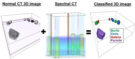
2.1. Principle of Sp-CT
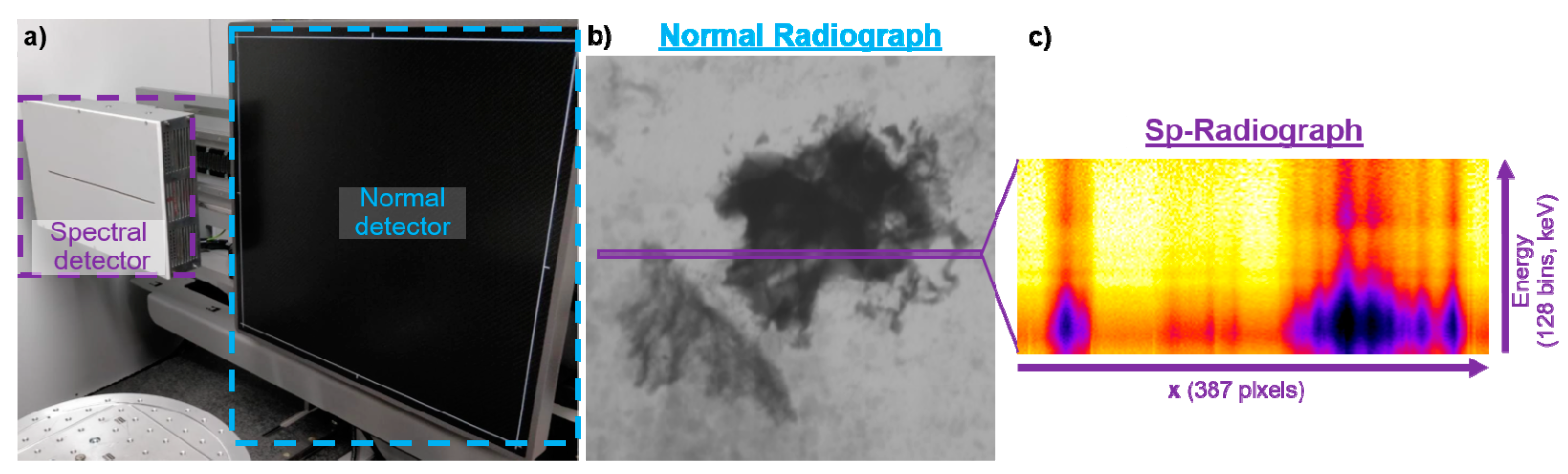
The X-rays of most commercial CT scanners are generated by a tungsten target that emits polychromatic X-rays with energy spectra similar to Figure 1a. Typically, the amount of X-rays generated decreases exponentially as a function of energy, except around the main emission energy of tungsten (59 keV). Commercial scanners allow control over the maximum energy of emitted X-rays, and by using filters (typically metallic plates) the lower energy X-rays can be removed to some extent. Nevertheless, these options offer the users little control over how many X-rays are emitted at specific energies, which makes the final X-ray energy spectra emitted by the source difficult to predict [11,14]. Furthermore, these X-rays are attenuated as they pass through a sample (Figure 1c,d) and the extent of the attenuation depends on the sample’s composition (µ, attenuation coefficient, which is a property of each material for each X-ray energy) and the cross-section along the X-ray path (l) is given by the Lambert–Beer’s law (Equation (1), where T is the transmission through the sample). To complicate the interpretation of the attenuation spectra, every element has a specific K-edge energy at which the attenuation increases suddenly (for gold, note the sudden increase of attenuation in Figure 1d and the decrease of transmission in Figure 1b at around 81 keV [22]). X-rays whose energy is matching a K-edge are absorbed by electrons from the inner electronic sphere of an atom causing its ejection from the atom. In conclusion, deriving mineral compositions from the total X-ray transmission that reaches the detector is difficult and may be misleading, especially in the case of heterogeneous samples with complex texture.
ln T = −µ.l,
Typical X-ray detectors used in CT scanners measure the total number of X-rays hitting a pixel, independently from their energy, i.e., the area under the curve of the transmitted energy spectrum (Figure 1b, top). The spectral detector used in this study allows resolving the amount of X-rays within 128 bins of energy between 20 and 160 keV [15]. For illustrative purposes, only 15 out of 128 bins of energy are exemplified in Figure 1b. In the given example, the energy spectrum of the transmitted X-rays allows distinguishing radiation that passed through gold or quartz. Even without preliminary knowledge about the sample, it would be possible to be sure about the presence of gold since the measured K-edge at 80.7 keV is specific to gold. Nevertheless, since silicon and oxygen have K-edges < 20 keV, one would not be able to classify a phase as quartz from the spectrum alone. Note that, since the relation between transmission and energy is exponential, X-rays with energies smaller than 20 keV are not transmitted through thicker samples; thus, the detection of elements with K-edges bellow 20 keV would not be practical using transmission X-ray techniques. Details about the signal measured by this detector can be consulted in [15].

2.2. Equipment

All scans presented in this study were performed with the TESCAN CoreTOM (TESCAN - XRE, Ghent, Belgium). The system is equipped with an X-ray source with a tungsten target capable of generating polychromatic X-rays up to 180 keV. The standard imaging detector is an amorphous Si flat panel with an active area of 428.4 by 428.4 mm² and containing a matrix of 2856 by 2856 pixels. Apart from the standard imaging detector, the CoreTOM is also equipped with a photon-counting line sensor, the TESCAN PolyDet (TESCAN-XRE, Ghent, Belgium), which can automatically slide in front of the standard detector. The PolyDet is a CdTe X-ray line detector with a sensor width of 307 mm composed of one row of square pixels 0.8 × 0.8 mm [15]. The direct detection sensor has an energy range from 20 up to 160 keV and can discriminate up to 128 energy bins for each of the 387 pixels that represent the horizontal field of view.
Acquila reconstruction 1.0.0.70 was used to reconstruct radiographs from the normal detector into 3D images using a cone beam filter back projection algorithm. The data from the PolyDet detector were reconstructed using the spectral fan beam reconstruction module in the Acquila reconstruction (TESCAN - XRE, Ghent, Belgium).

2.3. How It Works in Practise

The sample is initially scanned with a traditional X-ray detector without any particular difference from traditional CT. From the reconstructed 3D image or from the radiographs, slices of interest can be chosen, for example, slices crossing multiple dense phases that cannot be distinguished using normal CT. The plane to be scanned using the sp-detector is aligned with the centre of the source, Figure 2. If the elements to be detected are known, the maximum energy input and the filter used could be chosen in order to optimize the emitted spectrum, i.e., to maximize the detection of specific K-edge energies. The power, exposure time and number of averages are adjusted relative to the count rate and to minimize noise. Due to the lesser number of pixels in the sp-detector, for the same field of view, the pixel size of the reconstructed spectral images is 7.3 times higher (worse resolution) than the voxel size of the same slice reconstructed from the normal detector available in the CoreTOM and as measured on the cross-section of samples with known diameter.
If the material to be identified is large enough, and its spectrum can be isolated from the remaining sample, then a single radiograph may be sufficient to identify the material. This will be demonstrated in this work in experiment 1. However, this is usually not the case in rocks, where grains are dispersed in complex matrixes and can be too small to be localized in a radiograph. In this case, a 360 degrees scan is necessary, where spectrum radiographs are collected at regular angular intervals and later reconstructed as a 2D slice. In practise, the same slice is reconstructed 128 times, one per energy bin. This will be demonstrated in this work in experiment 2. The result is that the grey-value of each voxel in a slice corresponds to the attenuation coefficient of the material. Since the attenuation coefficient at specific energies is material-specific, the classification of the voxel is easier than using only grey-scale information that is proportional to the total X-ray attenuation (X-rays of all energies as measured by traditional CT) that is not only dependent on the material.

2.4. Experimental Conditions

The experiments presented in this study intend to demonstrate the potential use of sp-CT in two scenarios where classification using chemical information from the new spectral detector adds value to traditional total X-ray attenuation-based CT. The experiments were designed to provide the framework from where specific applications can be developed, rather than to provide an exhaustive study of the individual applications. Two experiments were conducted to test sp-radiographs, to classify mineral particles (Experiment 1), and to distinguish mineral phases containing gold, lead and/or antimony within a mineralised drill core (Experiment 2).
Experiment 1: The sample consists of 7 grains, two of galena (PbS), two of micro-porous ceria (CeO2), two of barite (BaSO4) and one of parisite (Ca1.1(Ce.9,La.5,Nd.3,Pr.1,Y.1,Sm.1)(CO3)3F1.7), embedded in epoxy resin within a cylindrical plastic tube with 15 mm diameter. The grains of galena, barite and parasite are from natural sources and may contain trace amounts of other elements. The chemical formula of parasite was obtained using microprobe. CeO2 was obtained by sintering of CeO2 powder at 1600 °C [23]. These samples were chosen in order to exemplify minerals containing elements with a K-edge covering the energy range detectable by the sp-detector, similar K-edge values (Ba and Ce), porous samples that have an artificial lower overall attenuation that makes them difficult to identify (ceria), and two materials containing the same main element (ceria and parasite). The sample was first scanned using traditional CT; second, each grain was radiographed using sp-radiography; third, the radiographies of each grain were matched with their 3D images for comparison of the spectra and gray-values. The following scanning conditions were used for the traditional CT scan: 180 keV, 16 W, 0.9 s, voxel size 16.6 μm, 1 mm Cu filter, and for the sp-radiographs: 120 keV, 30 W, 0.1 s, voxel size 18 μm, 0.1 mm Cu filter. Sp-radiographs were measured by the average of 10 spectra to reduce noise, and each spectrum was normalized to the flat field spectra that was measured at the beginning of the scan using 30 averages.
Experiment 2: The sample consisted of a half HQ core with 63.5 mm diameter from a West African orogenic Au deposit. The core is intersected by a 10–20 mm wide quartz-carbonate vein containing minor sulphosalts and gold grains. The host rock comprises silica-sericite-Fe carbonate and altered greywacke with pervasive auriferous pyrite (FeS2)-arsenopyrite (FeAs2) mineralisation. The core was first scanned using traditional CT; second, five height positions were scanned with sp-CT; third, the core was cut and polished into thin sections, which were analysed by quantitative mineral liberation analysis (MLA); fourth, the images were correlated for the purpose of identifying the same grains in the different imaging techniques as marked in Figure A2, i.e., normal CT identifies the grey-values, the sp-CT identifies possible heavy elements and the MLA determines which mineral corresponds to specific spectra and grey-values.
In the first step, the traditional CT scanning conditions were 180 keV, 18 W, 3.2 s, voxel size 18.7 μm, 1 mm Cu and 0.8 mm stainless steel filters. The resolution was sufficient to visualise the vein morphology and to determine the volumes containing the majority of gold-sulphosalt mineralisation. In the second step, the scanning conditions with sp-CT were 180 keV, 80 W, 0.1 s, voxel size 82 μm and 0.2 mm stainless steel filter. Each sp-radiograph (at each angle) was measured by the average of 10 spectra to reduce noise, and each spectrum was normalized to the flat field spectra that was measured at the beginning of the scan using 30 averages. Sp-CT scans with these conditions are under 7 min.
In the third step, the mineralogy of the sample is analysed to identify the minerals that contain elements detectable by sp-CT. For this purpose, three thin sections parallel to the long axis of the half core were prepared with a polishing fineness of 10 nm with colloidal silica. The thin sections were analysed using standard MLA procedures [24] that combine X-ray spectra mapping and backscatter image analysis (GXMAP mode). The analysis was complemented by higher spatial resolution analysis within grains of interest using sparse liberation analysis (SPL-LT mode). Scanning electron microscopy (SEM) X-ray conditions for the analysis were 25 kV, acceleration voltage, 10 nA probe current, 5.6 μm spot size. The settings for GXMAP were pixel size 2 μm and resolution (pixels) 500 × 500 μm for the backscatter image, which was combined with a spectra map that has a step size of 6 μm and an acquisition time of 7 ms. The settings for SPL-LT were pixel size 0.25 μm and resolution (pixels) 2000 × 2000 μm for the backscatter image, which was combined with a spectra map with the same resolution of the GXMAP. Datasets were processed with the FEI MLA suite software. GXMAP analysis of the vein composition identified the minor phases as the sulphosalts boulangerite (Pb5Sb4S11) and tetrahedrite ((Cu,Fe)12Sb4S13) plus agglomerations of large arcuate gold grains (250–500 μm). Numerous smaller gold grains (<50 μm) are composed of gold with high fineness (<10% Ag). The morphology of gold grains is typical of fluid un-mixing due to depressurisation during vein formation [25,26].

3. Results

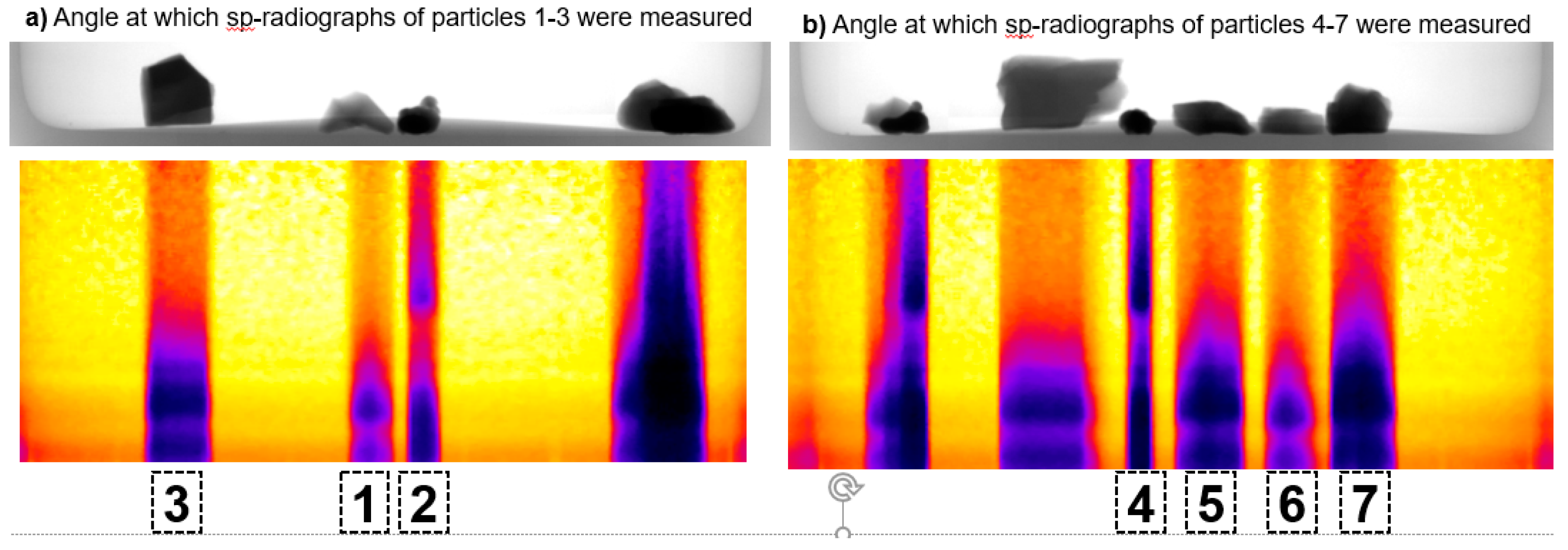
3.1. Spectral Radiographs

The grey-value of voxels in 3D images obtained using CT is often not only a function of the material chemistry, but also depends on artefacts, porosity, uneven shape and position within the field of view [27]. These effects can hinder the accurate classification of particles based only on the grey-scale. Experiment 1 exemplifies a scenario where particles could not have been classified correctly, even though we know how many particles of each mineral are present, without the additional chemical information from spectrum radiographs. For example, despite the fact that 4 phases are present, only 3 classes of particles can be distinguished from the grey-scale in Figure 3a (high attenuation, class 1: particles 2, 4 and 7; medium attenuation, class 2: particles 1, 3 and 5; low attenuation, class 3: particle 6). Due to the distinctive grey-scale, one would instinctively classify particle 6 as parisite because it is the only mineral with a single particle in the sample (other minerals are represented by two particles in the sample). This would have been a wrong classification since that particle is barite. The reason that the barite particle is less attenuating than the other barite particle is its position. Since the particle is shielded between other dense particles the X-rays going through the barite are harder (X-rays with higher energies are less attenuated than lower energy X-rays) than those going through the other barite particle 1. The porosity within CeO2 particles also makes them less attenuating than what would be expected from their high density. Therefore, the grey-scale of porous CeO2 (density without pores = 7.22 g.cm−3) particles cannot be distinguished from the grey-scale of barite and parisite (densities in the range 4.3 to 4.5 g.cm−3).
Spectral radiographs at two angles were measured to determine the spectra of individual particles (Figure A1). The radiograph from the first angle is shown in Figure 3b, which was used to measure the spectra of particles that are not aligned between the source and the detector. The second angle was necessary to measure the spectra of particles 1 and 2 that are aligned at the first angle (Figure 1b); thus, the spectra would contain information from both particles. In Figure 3c, it is noticeable that the drop of transmission at the K-edge of any element is spread over about 10 energy bins (~11 keV), which makes it difficult to attribute a specific K-edge energy directly from transmission plots. Nevertheless, the derivative of the transmission was shown to provide a better perspective over the variation of transmission nearby the K-edge energy. The minimum values correspond to the most accentuated decrease in transmission, which is expected to occur at the K-edge. This is observed valid within the energy interval of one energy bin, 1.1 keV. The two galena particles are clearly the most attenuating and show a distinctive drop in transmission at the K-edge energy of lead, 89 keV (red lines and red particles in Figure 3d). The K-edge of barium (38 keV) and cerium (40.4 keV) can be clearly distinguished, e.g., the blue and green lines. Consequently, barite can be clearly distinguished from cerium containing minerals. Less distinctive are the differences between ceria and parisite. It can be argued that the increase of attenuation at energies just above the K-edge of cerium increases slower than at energies just below the K-edge (purple line), which is unexpected and contrary to the progression observed for the other minerals. This could indicate the presence of other rare earth elements with K-edges similar to cerium known to be present in small but detectable amounts in the parasite mineral structure, e.g., La, Nd, Pr, Y, Sm as mineral lattice substitutes of Ce. The weak signal from these elements is further shielded by the variabilities of transmission around 59 keV, which corresponds to the emission edge of tungsten. It is possible that small variations at the source (whereby the target is made of tungsten) can reduce the sensitivity of the technique around the emission edge energies of tungsten, especially to detect trace elements.
To conclude, the X-ray transmission spectrum through individual particles can be directly measured in a quick spectrum radiograph. A measurement time of 1 s (exposure time of 100 ms per radiograph multiplied by 10 radiographs that are used to calculate one average radiograph) is sufficient to obtain a spectrum with a reasonable high signal to noise ratio (Figure 3b,c). Note that sp-radiographs can only be used to classify particles that are not enclosed by a matrix that contains elements with K-edges above 20 keV. For example, if two particles are aligned between source and the detector (e.g., particles 1 and 2 in Figure 3b) the mixed spectra would be difficult to interpret, thus a full scan would be necessary, as performed in experiment 2.

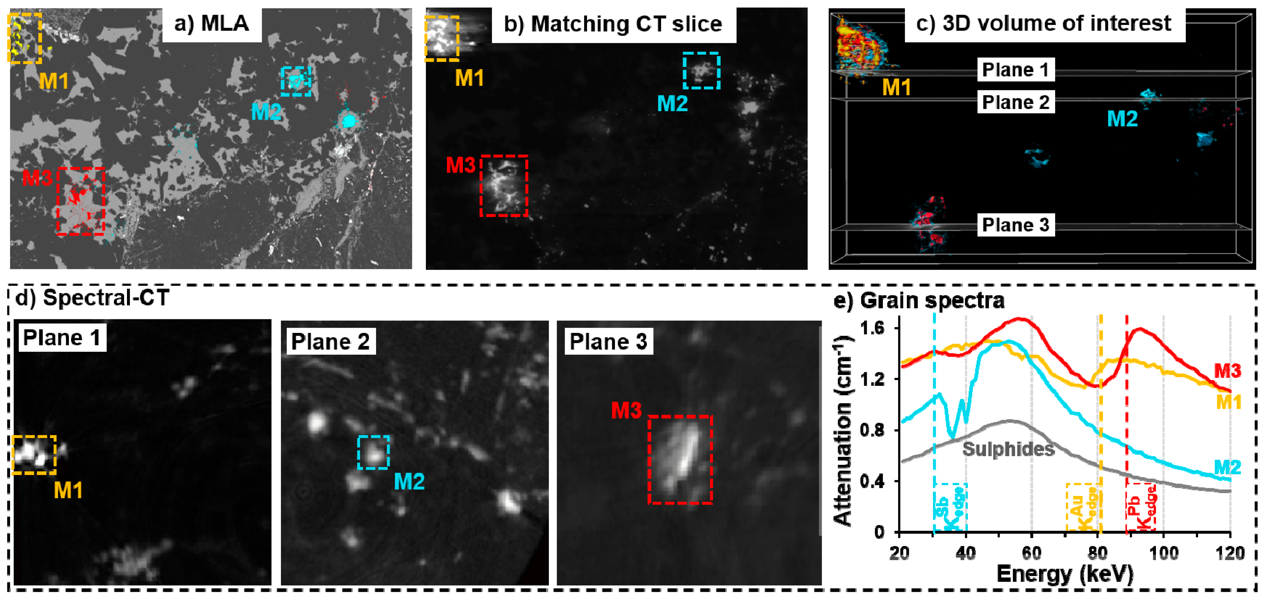
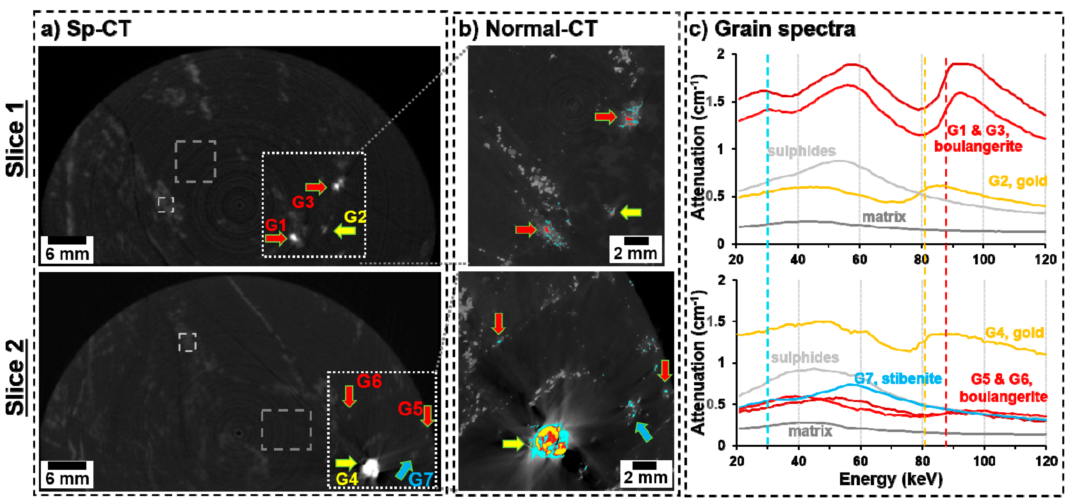
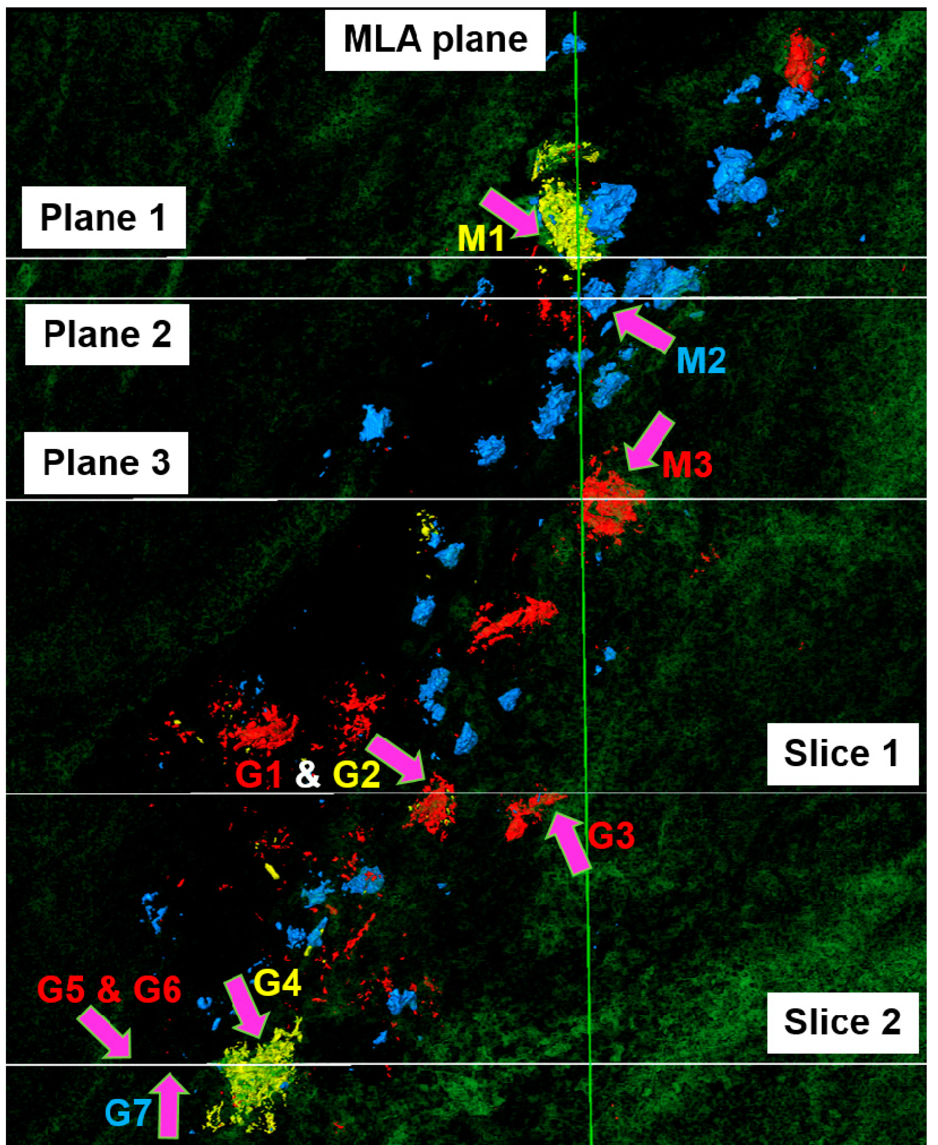
3.2. Spectral Tomography

Experiment 2 demonstrates the potential of using the reconstructed spectrum of voxels to classify mineral phases in specific slices of a 3D image (Figure 4). MLA analysis showed that the main minerals containing elements with K-edges within the measurable energy range 20–160 keV present in the deposit are: gold, Au (yellow, grain M1); tetrahedrite, (Cu,Fe)12Sb4S13 (blue, grain M2); and boulangerite Pb5Sb4S11 (red, grain M3). Other heavy sulphides such as arsenopyrite (white in MLA image), light sulphides such as pyrite (light grey), and the rock matrix of silicates, carbonates and phosphates (dark grey) were also identified. Most of these phases could not be distinguished using normal CT as they have overlapping ranges of grey-values for different minerals. The overlap is mostly due to the variable grain size and associated partial volume effects, in addition to imaging artefacts such as beam hardening. To distinguish the three denser phases using the K-edge signal from Sb, Pb and Au, the three grains M1-M3 were analysed by MLA, CT and Sp-CT (Figure 4). The representation of the grains intercepted by the different techniques shown in Figure 4a,b,d is represented in Figure 4c (see positions relative to the entire sample in Figure A2). The typical spectra from tetrahedrite, boulangerite and gold measured for the grains M1-M3 are shown in Figure 4e. Note that the classification given by MLA validated the minerals of M1-M3 (Figure 4).
Information from the spectra of the grains M1-M3 was used to classify other grains (e.g., G1–G7) where MLA information is not available (Figure 5). Several interesting observations can be drawn from the spectra of the grains G1–G7. The K-edge of Pb is detected in G1, G3, G5 and G6 (red arrows). From the MLA analysis, the main mineral that contains Pb is boulangerite which also contains Sb. However, only G1 and G3 show the K-edge of Sb, and G5 and G6 show a continuous spectrum below 40 keV, thus without evidence of the Sb K-edge. One could speculate that G5 and G6 are lead phases that do not contain Sb and that were not identified by MLA. Nevertheless, G5 and G6 could indeed be boulangerite but the grains are too small to detect the Sb signal. This is supported by the lower total attenuation of G5 and G6. Since the drop of attenuation at the K-edge of Sb is about 4 times smaller than at the K-edge of Pb and the signal from the K-edge of Pb is small, the signal of Sb in G5 and G6 would be at the level of noise. Nevertheless, normal CT shows that the grey-scale of G5 and G6 matches the grey-scale expected for tetrahedrite (blue), e.g., G5-G7 have a similar grey-scale, Figure 5b. However, the spectrum signal is clearly different (Figure 5c). G7 shows a depression after 30 KeV indicating the presence of Sb, and a continuous signal around 88 KeV, which indicates that Pb is not present.
Distinguishing gold grains from grains containing lead phases is a primordial challenge in ore characterization by CT. Even though gold has a significantly higher attenuation than lead sulphides, such as boulangerite and galena, the grey-scale range representing these minerals are usually overlapping. That is mostly due to the partial volume effect due to the typically smaller size of gold grains. For example, G2 has an attenuation lower than G1 and G3, thus classifying G2 only based on the grey-scale would incorrectly label the grain as a phase less attenuating than boulangerite, Figure 5b. In fact, G2 shows the presence of a K-edge at 81 keV, which corresponds to gold, similar to G4 that has a much higher total attenuation, Figure 5c. Thereafter, it can be concluded that even though G2 and G4 have similar compositions, since the size of G2 is close to the voxel size, its total attenuation is affected by partial volume effects, and thus it could not be correctly classified using traditional CT. We highlight that the position of the K-edge remains the same in the different spectra, which allows identifying the main elements, despite the overall attenuation being different because of the size and shape of the grains.

3.3. Applications and Limitations

The spectral techniques presented here follow an approach similar to that used for automated mineralogical classification of surfaces using SEM-based methods [28], i.e., combining grey-scale images and chemical information from spectra. The main difference is that in tomographic techniques the chemical signal has to pass through the sample (transmitted X-rays) before it is measured. A direct benefit is that bulk information can be acquired without the need of sample preparation. Although, the energy and the spatial resolutions are worse than those possible using SEM-based surface techniques. Furthermore, only harder X-rays (e.g., energies above 20 keV) can escape the sample, thus only heavier elements can be identified from the detection of their K-edge signal. Nevertheless, sp-CT and sp-radiography can offer a quick chemical evaluation of which heavy elements are present inside a sample, which is an important complement to a fundamental limitation of traditional CT, especially on its application to study complex Earth materials.
Despite the possibility of a quick chemical evaluation, the result of an sp-CT scan corresponds only to a 1-voxel thick section of a sample. It is possible to scan consecutive sections of a sample that can then be stacked into larger volumes as a multidimensional image where each voxel contains not only a grey-value but a full energy spectrum. The combination of a higher resolution 3D image from traditional CT with a 3D image from sp-CT, results in a high-resolution multidimensional image (3D + grey-value + energy spectrum). While the high-resolution image can be used to define the grains with better accuracy, the energy spectrum can be used to improve the classification of the grain, i.e., better classification than if using only the grey-scale. The ultimate goal of using this strategy is to achieve automatic classification of phases using the grey-scale, the element information from K-edge positions and the overall energy spectrum, similar to how it is done when using SEM-based automated mineralogy on surfaces without requiring sample preparation and without the 2D stereological bias [29].
The key limitation of using the 3D sp-CT method described in the previous paragraph is the time necessary to measure large samples. For example, it is estimated that over 600 sp-CT scans would be necessary to scan the 5.1 cm length of the sample core used in experiment 2, which would require over 2 days to scan the entire sample. This is unacceptably long to implement 3D sp-CT as a common tool for research and more so for industry. While future developments of detector technology may enable faster scans, with the available technology, alternative protocols and software development for automation and integration of data from sp-CT and traditional CT could reduce the time necessary to classify 3D images. Three possible developments are envisaged. First, many grains are sufficiently large so that some slices could be scanned with larger voxel size, i.e., broader vertical sections can be analysed in single scans. Second, many slices of the core do not cross minerals containing elements with a K-edge in the detectable range, >20 KeV. Such minerals typically have an attenuation higher than the rock matrix in the normal CT image. Therefore, a pre-selection of the slices of interest and resolution of the scan could be done using a preliminary analysis of the high-resolution CT image. Third, if grains are sufficiently large, e.g., diameter > 1 mm, classification of a grain within the core could be achieved using sp-radiographs, similar to experiment 1 shown in this work. This would, however, be limited to individual grains for which the x-rays can cross the sample without intercepting other minerals containing elements with a detectable K-edge. In conclusion, chemical information should only be measured in specific positions where the information is necessary and the measuring parameters should be adjusted to the material to be characterized, e.g., according to chemistry and grain size.
It is estimated that the full characterization of the same core sample could be achieved with as few as 52 sp-CT scans at predefined positions. This would reduce the scanning time to under 6 h, which would be a competitive time when compared to, for example, SEM-based surface characterization that requires extensive thin section preparation and ultimately may only measure an unrepresentative section of the sample. Nevertheless, currently the decision about which slices should be scanned must be done manually by an operator, which is even more time consuming than scanning the 600 sections necessary to analyse the entire core. Therefore, a selective slice analysis would require a software capable of easing the selection of the positions and resolutions of scans based on the presence and size of the grains within a slice as measured in a traditional 3D CT image. Active learning could be a potential method to automate the decision of pre-selecting the optimal slices to scan [30].
A simpler application of spectral information consists of determining the grey-scale ranges representing mineral phases in traditional 3D CT images by using information from sp-CT. The grey-scale range representing a mineral or a group of minerals containing a specific element could be identified on just some slices, and then extrapolated to the rest of the sample. This is exemplified in Figure 6 where gold (yellow), boulangerite (red) and tetrahedrite (blue) grains are found mostly within the following ranges of grey-values gold, [15,311; 65,535], boulangerite [7503; 15,310] and tetrahedrite [5243; 7502]. A similar classification method where the specific grey-scale of mineral groups was calibrated using SEM-based analysis was shown possible [7,31,32], although the method was very time consuming. This method can give wrong classification in regions where the grey-values are affected by imaging artefacts, e.g., around denser grains, and partial volume effects, e.g., small grains.
To avoid defining grey-value ranges for specific phases, spectral information could also be used to classify a small number of slices of a traditional 3D CT image, which can then be used to train deep learning segmentation models. Such models can then be applied to all slices of the sample’s 3D image and to other similar samples, to automatically recognize and segment the phases of interest. The training slices must include microstructures that are representative of the whole sample, thus the amount of scans necessary to train a reliable and predictive deep learning model depends on the complexity of the sample. Therefore, for simple microstructures, sp-CT-based 3D mineralogical classification could be faster than 2D surface characterization methods that require sample preparation, especially if a large number of samples with similar mineralogical composition is to be analysed.
The ability to classify mineral phases in 3D images by combining grey-scale and energy spectra information would bolster the applicability of 3D imaging for materials characterization in the Earth sciences. This would, of course, be limited to the classification of grains with appropriate size and phases with a composition that can be identified using X-ray transmitted spectra. For example, the characterization of ore minerals for which the grains are often sufficiently large and contain heavy elements. It is anticipated that the technique can be extensively applied to research in economic geology, such as ore formation, where the mineral distribution in veins can be quantified, and in minerals processing engineering, where the 3D properties of ore particulates can be measured at different stages of comminution, separation and leaching.

4. Conclusions

Spectral CT and spectral radiographies help classify mineral phases in 3D images by combining the high spatial resolution and grey-scale of normal CT images with the attenuated energy spectra that gives information about the elements in a phase. Adding chemical information to the overall attenuation of a phase is expected to improve mineral classification, which can bolster the applicability of 3D imaging for materials characterization in the Earth sciences. This would, of course, be limited to the classification of grains with appropriate size and elemental composition, i.e., with a K-edge that can be identified using X-ray transmitted spectra. For example, the characterization of ore minerals for which the grains are often sufficiently large and contain heavy elements (heavier than silver). This can be particularly interesting for research in economic geology, such as ore formation, where the mineral distribution in veins can be analysed, and in minerals processing engineering, where the 3D properties of ore particulates can be measured at different stages of comminution, separation and leaching.

Author Contributions

Conceptualization, J.R.A.G., M.A.B. and A.D.R.; methodology, J.R.A.G. and G.W.-H.; software, J.R.A.G. and M.A.B.; formal analysis, J.R.A.G. and G.W.-H.; writing—original draft preparation, J.R.A.G.; writing—review and editing, J.R.A.G., G.W.-H., M.A.B. and A.D.R.; visualization, J.R.A.G. and G.W.-H.; funding acquisition, A.D.R. All authors have read and agreed to the published version of the manuscript.

Funding

This research has received funding from the European Institute of Innovation and Technology (EIT). This body of the European Union receives support from the European Union’s Horizon 2020 research and innovation programme.

Data Availability Statement

The data presented in this study is stored in RODARE, the data repository of HZDR. Access to the data will be open access once the article is published.

Acknowledgments

The authors would like to thank Sabine Gilbricht for assistance with the MLA analyses at TUBAF. In addition, we would like to acknowledge Barrick Gold Corporation for their support and provision of the drill core sample.

Conflicts of Interest

The authors declare no conflict of interest.

Appendix A

Figure A1. Radiographs at angles where the marked particles are not aligned between source and detector (a) particles 1–3 and (b) particles 4–7. At these positions, the attenuation spectra of the marked particles are independent from the other particles. These positions were used to derive the spectra in Figure 3c.
Minerals 11 00598 g0a1
Figure A2. 3D volume of interest from the scanned field of view of experiment 2. The planes and slices scanned with the spectrum detector (white, horizontal) as analysed in Figure 4 and Figure 5, the vertical cut that was analysed by MLA (green line), as well as the grains of interest indicated by pink arrows (M, identifies grains studied by MLA and Sp-CT, and G, identifies grains studied only by Sp-CT). Light phases (e.g., silicates) are set transparent, green are light sulphides (e.g., pyrite), yellow are very bright voxels (mostly gold), red voxels have the second brightest intensity range (mostly Pb sulphides), blue voxels have the third brightest intensity range (mostly Sb and As sulphides).
Minerals 11 00598 g0a2

References

  1. Withers, P.J.; Bouman, C.; Carmignato, S.; Cnudde, V.; Grimaldi, D.; Hagen, C.K.; Maire, E.; Manley, M.; Du Plessis, A.; Stock, S.R. X-ray computed tomography. Nat. Rev. Methods Primers 2021, 1, 18. [Google Scholar] [CrossRef]
  2. Cnudde, V.; Boone, M.N. High-resolution X-ray computed tomography in geosciences: A review of the current technology and applications. Earth Sci. Rev. 2013, 123, 1–17. [Google Scholar] [CrossRef] [Green Version]
  3. Guntoro, P.I.; Ghorbani, Y.; Koch, P.-H.; Rosenkranz, J. X-ray Microcomputed Tomography (µCT) for Mineral Characterization: A Review of Data Analysis Methods. Minerals 2019, 9, 183. [Google Scholar] [CrossRef] [Green Version]
  4. Wang, Y.; Lin, C.L.; Miller, J.D. Quantitative analysis of exposed grain surface area for multiphase particles using X-ray microtomography. Powder Technol. 2017, 308, 368–377. [Google Scholar] [CrossRef]
  5. Reyes, F.; Lin, Q.; Cilliers, J.J.; Neethling, S.J. Quantifying mineral liberation by particle grade and surface exposure using X-ray microCT. Miner. Eng. 2018, 125, 75–82. [Google Scholar] [CrossRef]
  6. Reyes, F.; Lin, Q.; Udoudo, O.; Dodds, C.; Lee, P.D.; Neethling, S.J. Calibrated X-ray micro-tomography for mineral ore quantification. Miner. Eng. 2017, 110, 122–130. [Google Scholar] [CrossRef] [Green Version]
  7. Godinho, J.; Kern, M.; Renno, A.D.; Gutzmer, J. Volume quantification in interphase voxels of ore minerals using 3D imaging. Miner. Eng. 2019, 144, 106016. [Google Scholar] [CrossRef]
  8. Miller, J.D.; Lin, C.L. X-ray tomography for mineral processing technology—3D particle characterization from mine to mill. Miner. Metall. Process. 2018, 35, 1–12. [Google Scholar] [CrossRef]
  9. Miller, J.D.; Lin, C.-L.; Hupka, L.; Al-Wakeel, M.I. Liberation-limited grade/recovery curves from X-ray micro CT analysis of feed material for the evaluation of separation efficiency. Int. J. Miner. Process. 2009, 93, 48–53. [Google Scholar] [CrossRef]
  10. Gajjar, P.; Jørgensen, J.S.; Godinho, J.R.A.; Johnson, C.G.; Ramsey, A.; Withers, P.J. New software protocols for enabling laboratory based temporal CT. Rev. Sci. Instrum. 2018, 89, 93702. [Google Scholar] [CrossRef] [Green Version]
  11. Bam, L.; Miller, J.; Becker, M. A Mineral X-ray Linear Attenuation Coefficient Tool (MXLAC) to Assess Mineralogical Differentiation for X-ray Computed Tomography Scanning. Minerals 2020, 10, 441. [Google Scholar] [CrossRef]
  12. Fandrich, R.; Gu, Y.; Burrows, D.; Moeller, K. Modern SEM-based mineral liberation analysis. Int. J. Miner. Process. 2007, 84, 310–320. [Google Scholar] [CrossRef]
  13. Tuşa, L.; Kern, M.; Khodadadzadeh, M.; Blannin, R.; Gloaguen, R.; Gutzmer, J. Evaluating the performance of hyperspectral short-wave infrared sensors for the pre-sorting of complex ores using machine learning methods. Miner. Eng. 2020, 146, 106150. [Google Scholar] [CrossRef]
  14. Pankhurst, M.J.; Fowler, R.; Courtois, L.; Nonni, S.; Zuddas, F.; Atwood, R.C.; Davis, G.R.; Lee, P.D. Enabling three-dimensional densitometric measurements using laboratory source X-ray micro-computed tomography. SoftwareX 2018, 7, 115–121. [Google Scholar] [CrossRef]
  15. Sittner, J.; Godinho, J.R.A.; Renno, A.D.; Cnudde, V.; Boone, M.; de Schryver, T.; van Loo, D.; Merkulova, M.; Roine, A.; Liipo, J. Spectral X-ray computed micro tomography: 3-dimensional chemical imaging. X-Ray Spectrom 2021, 50, 92–105. [Google Scholar] [CrossRef]
  16. Rebuffel, V.; Tartare, M.; Brambilla, A.; Moulin, V.; Verger, L. Multi-energy X-ray Techniques for NDT: A New Challenge. In Proceedings of the 11th European Conference on Non-Destructive Testing, Prague, Czech Republic, 6–10 October 2014. [Google Scholar]
  17. Roessl, E.; Cormode, D.; Brendel, B.; Jürgen Engel, K.; Martens, G.; Thran, A.; Fayad, Z.; Proksa, R. Preclinical spectral computed tomography of gold nano-particles. Nucl. Instrum. Methods Phys. Res. Sect. A Accel. Spectrom. Detect. Assoc. Equip. 2011, 648, S259–S264. [Google Scholar] [CrossRef]
  18. Cuadros, A.; Ma, X.; Arce, G.R. Compressive spectral X-ray tomography based on spatial and spectral coded illumination. Opt. Express 2019, 27, 10745–10764. [Google Scholar] [CrossRef] [PubMed]
  19. Alves, H.; Lima, I.; Lopes, R.T. Methodology for attainment of density and effective atomic number through dual energy technique using microtomographic images. Appl. Radiat. Isot. 2014, 89, 6–12. [Google Scholar] [CrossRef]
  20. Egan, C.K.; Jacques, S.D.M.; Wilson, M.D.; Veale, M.C.; Seller, P.; Beale, A.M.; Pattrick, R.A.D.; Withers, P.J.; Cernik, R.J. 3D chemical imaging in the laboratory by hyperspectral X-ray computed tomography. Sci. Rep. 2015, 5, 15979. [Google Scholar] [CrossRef] [PubMed] [Green Version]
  21. Roessl, E.; Proksa, R. K-edge imaging in x-ray computed tomography using multi-bin photon counting detectors. Phys. Med. Biol. 2007, 52, 4679–4696. [Google Scholar] [CrossRef] [PubMed]
  22. Warr, R.; Ametova, E.; Cernik, R.J.; Fardell, G.; Handschuh, S.; Jørgensen, J.S.; Papoutsellis, E.; Pasca, E.; Withers, P.J. Enhanced Hyperspectral Tomography for Bioimaging by Spatiospectral Reconstruction. 2021. Available online: http://arxiv.org/pdf/2103.04796v1 (accessed on 10 March 2021).
  23. Godinho, J.R.; Piazolo, S.; Stennett, M.C.; Hyatt, N.C. Sintering of CaF2 pellets as nuclear fuel analog for surface stability experiments. J. Nucl. Mater. 2011, 419, 46–51. [Google Scholar] [CrossRef]
  24. Schulz, B.; Sandmann, D.; Gilbricht, S. SEM-Based Automated Mineralogy and Its Application in Geo- and Material Sciences. Minerals 2020, 10, 1004. [Google Scholar] [CrossRef]
  25. Groves, D.; Phillips, G.N.; Ho, S.; Houstoun, S.M.; Standing, C.A. Craton-scale distribution of Archean greenstone gold deposits; predictive capacity of the metamorphic model. Econ. Geol. 1987, 82, 2045–2058. [Google Scholar] [CrossRef]
  26. Sibson, R.H.; Robert, F.; Poulsen, K.H. High-angle reverse faults, fluid-pressure cycling, and mesothermal gold-quartz deposits. Geology 1988, 16, 551. [Google Scholar] [CrossRef]
  27. Lin, Q.; Neethling, S.J.; Dobson, K.J.; Courtois, L.; Lee, P.D. Quantifying and minimising systematic and random errors in X-ray micro-tomography based volume measurements. Comput. Geosci. 2015, 77, 1–7. [Google Scholar] [CrossRef] [Green Version]
  28. Hoal, K.O.; Stammer, J.G.; Appleby, S.K.; Botha, J.; Ross, J.K.; Botha, P.W. Research in quantitative mineralogy: Examples from diverse applications. Miner. Eng. 2009, 22, 402–408. [Google Scholar] [CrossRef]
  29. Ueda, T.; Oki, T.; Koyanaka, S. Experimental analysis of mineral liberation and stereological bias based on X-ray computed tomography and artificial binary particles. Adv. Powder Technol. 2018, 29, 462–470. [Google Scholar] [CrossRef]
  30. Kusne, A.G.; Yu, H.; Wu, C.; Zhang, H.; Hattrick-Simpers, J.; DeCost, B.; Sarker, S.; Oses, C.; Toher, C.; Curtarolo, S.; et al. On-the-fly closed-loop materials discovery via Bayesian active learning. Nat. Commun. 2020, 11, 5966. [Google Scholar] [CrossRef]
  31. Furat, O.; Leißner, T.; Ditscherlein, R.; Šedivý, O.; Weber, M.; Bachmann, K.; Gutzmer, J.; Peuker, U.; Schmidt, V. Description of Ore Particles from X-Ray Microtomography (XMT) Images, Supported by Scanning Electron Microscope (SEM)-Based Image Analysis. Microsc. Microanal. 2018, 24, 461–470. [Google Scholar] [CrossRef]
  32. Voigt, M.; Miller, J.A.; Mainza, A.N.; Bam, L.C.; Becker, M. The Robustness of the Gray Level Co-Occurrence Matrices and X-Ray Computed Tomography Method for the Quantification of 3D Mineral Texture. Minerals 2020, 10, 334. [Google Scholar] [CrossRef] [Green Version]
Figure 1. Example of the polychromatic nature of the X-ray spectrum emitted by the tungsten source of the CoreTOM scanner (a), and the spectrum transmitted through a sample of quartz (dark grey) or gold (light grey) (b). As schematized in (c), changes between emitted and transmitted X-rays take place in the sample. The simulated relation between X-ray attenuation and energy taking place across a gold or quartz sample is shown in (d). Note that the spectral detector measures the X-rays within discretized bins of energy while a normal detector only measures the total amount of X-rays at all energies (area under the curves).
Minerals 11 00598 g001
Figure 2. Schematics of the experimental setup (a), with an example of a typical normal radiograph (b) and an sp-radiograph (c). Note that the spectral detector can be moved in and out of the front of the normal detector and is aligned to measure precisely at the centreline.
Minerals 11 00598 g002
Figure 3. Classification of particles in a grey-scale 3D image (a) using spectral radiographs of individual particles (b). Note the correlation between the normal radiograph (grey) and the spectral radiograph (colour). The transmission spectrum and its derivate corresponding to individual particles are shown (c). Numbers and colours identify specific mineral phases that are correlated to classify the particles in the 3D images (d). The grey-scale in (a) is based on the total attenuation after a normal CT scan. Spectral plots are averaged values from all pixels representing each particle. Note that the spectra of some particles overlap in the example sp-radiograph shown; however, the data for the plots were taken from positions where the particles are not aligned (see Figure A1).
Minerals 11 00598 g003
Figure 4. Three grains (M1-M3) classified by (a) MLA with the same grains represented in the (b) CT image (2D plane matching the MLA image) and (c) 3D view of the volume of interest. (d) The same grains imaged using Sp-CT on planes 1–3 that are perpendicular to the MLA image as marked in (c). (e) The measured spectra of grains M1-M3 and the sulphides matrix. Grain M1 (yellow) is identified by MLA and sp-CT as gold. Grain M2 (blue) is identified as tetrahedrite by MLA and the K-edge of Sb is identified. Grain M3 (red) is identified by MLA as boulangerite and the K-edge of both Sb and Pb are identified.
Minerals 11 00598 g004
Figure 5. Classification of individual grains (G1–G7) in sp-CT images (a), using the grey-scale from traditional CT (b), and using the spectra from individual grains obtained with sp-CT (c) on two different slices (experiment 2). The colour scale is based on the total attenuation. The slice of normal CT shown corresponds to the region of interest shown as a dotted box.
Minerals 11 00598 g005
Figure 6. 3D image of a subvolume of a vein rich in heavy elements classified using a combination of traditional CT and sp-CT. Light phases (e.g., silicates and carbonates) are set transparent, green denotes light sulphides (e.g., pyrite), yellow denotes gold grains, red denotes boulangerite grains, blue denotes tetrahedrite grains.
Minerals 11 00598 g006
Publisher’s Note: MDPI stays neutral with regard to jurisdictional claims in published maps and institutional affiliations.

