
Empirical Application of Generalized Rayleigh Distribution for Mineral Resource Estimation of Seabed Polymetallic Nodules


Abstract
1. Introduction
2. Three Hypotheses for an Idealized Model of Seabed Polymetallic Nodules
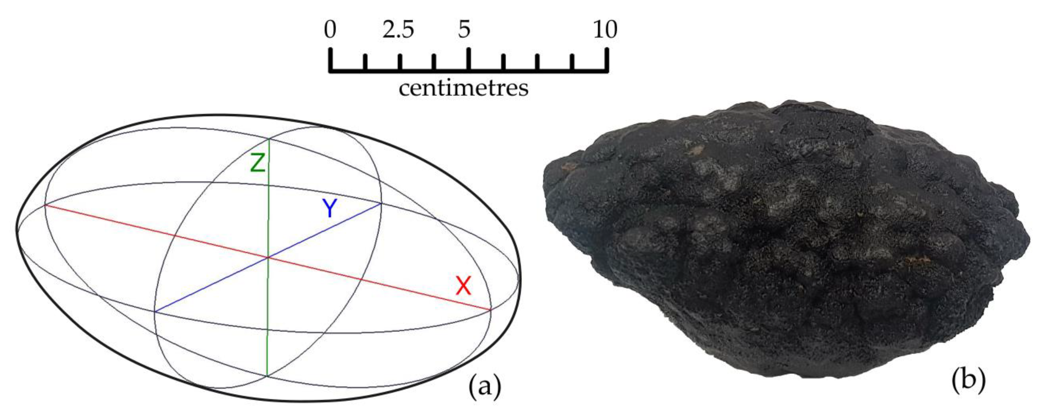
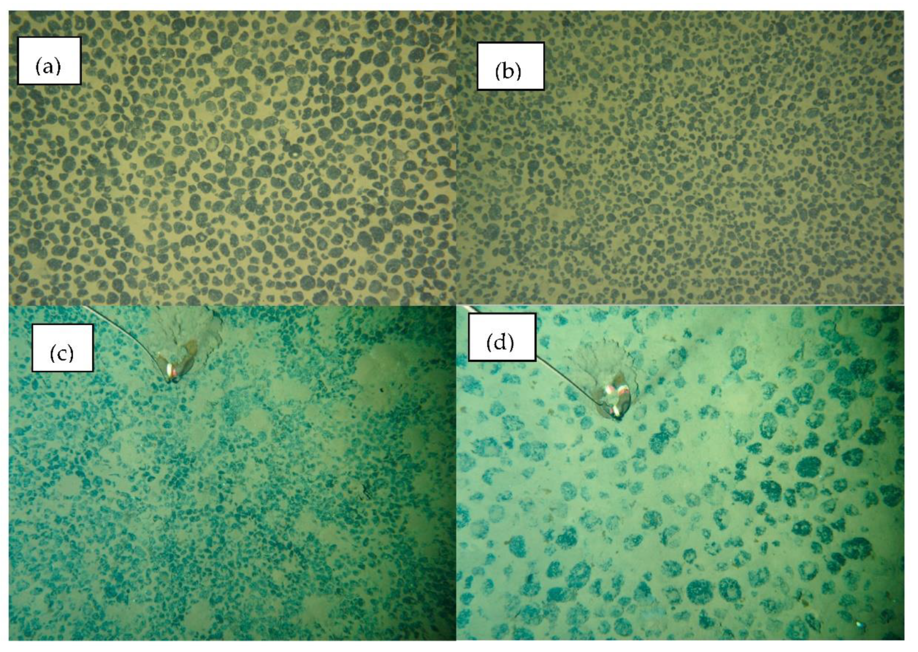
- Each nodules piece is of ellipsoidal shape (e.g., in Figure 2a,b), which is defined by its three axes , and , where , with being the number of nodules. Here is the long or major axis, which is usually in the horizontal plane while and are the two typically shorter minor axes in the horizontal and vertical planes.
- Within a certain boundary (domain) on the seabed, the ellipsoidal nodules are similar in shape, i.e., the ratio between two minor axes and the major axis, and are constant.
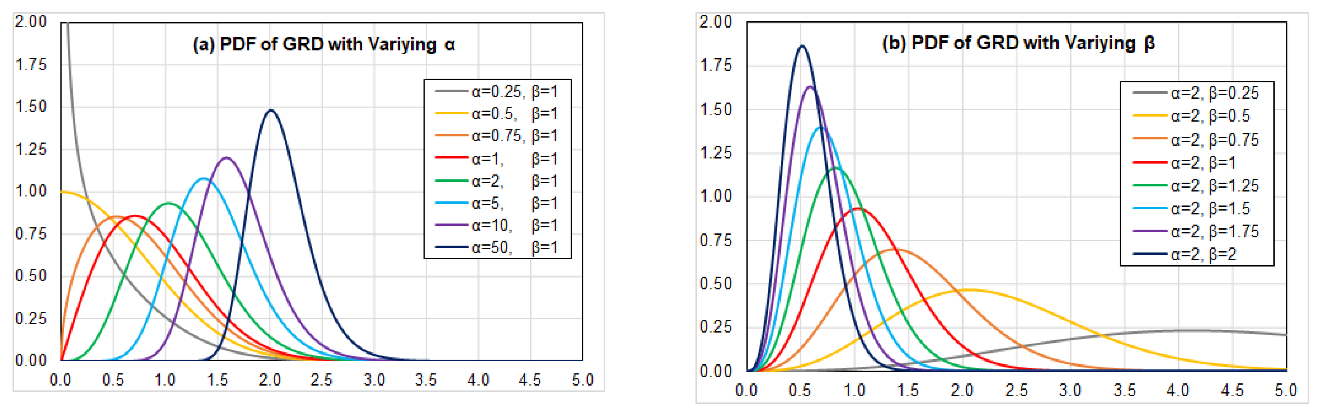
- Within a certain boundary (domain) on the seabed, the long axis of nodule follows a Generalized Rayleigh Distribution (GRD), which is defined by a pair of parameters α and β (See Section 3).
3. Generalized Rayleigh Distribution (GRD) and the Traditional Method
3.1. Mean and Standard Deviation of the Generalized Rayleigh Distribution (GRD)
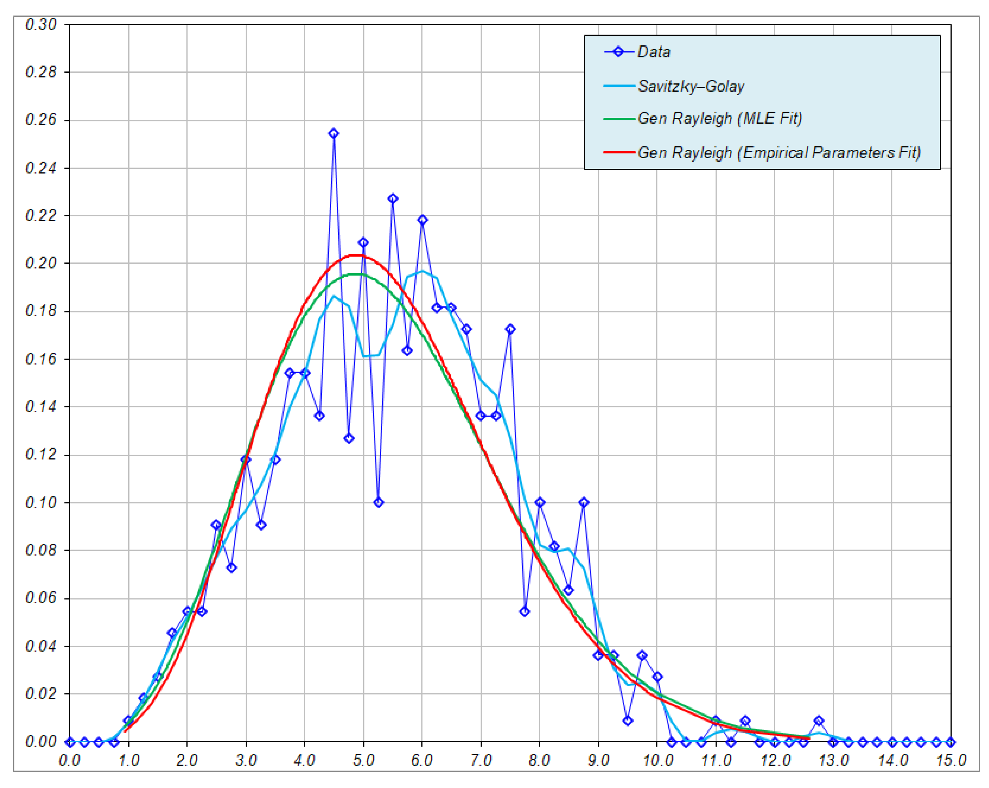
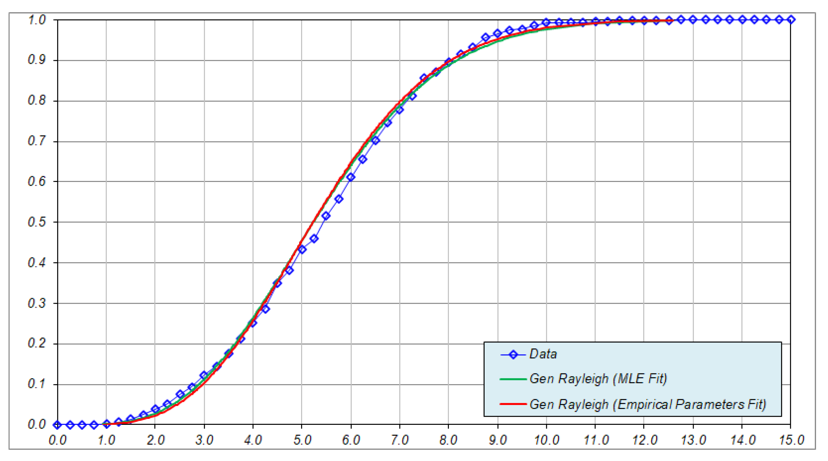
3.2. Test of Goodness-of-Fit of Generalized Rayleigh Distribution
3.2.1. Parameter Estimation by Maximum Likelihood Estimation (MLE)
3.2.2. The Anderson–Darling Test Statistics
3.2.3. The Test Criteria for Hypothesis
4. A New Empirical Method and Its Application to Nodule Resources
4.1. Empirical Estimation of Parameters of the Generalized Rayleigh Distribution
4.2. Resource Estimation for Seabed Polymetallic Nodules Using Coverage and Abundance
- The nodule is assumed to be in an idealized ellipsoid shape.
- Nodules within a certain boundary are assumed to be “similar” in shape, the ratios between the lengths of the two minor axes and the major axis (denoted by and ) are constant.
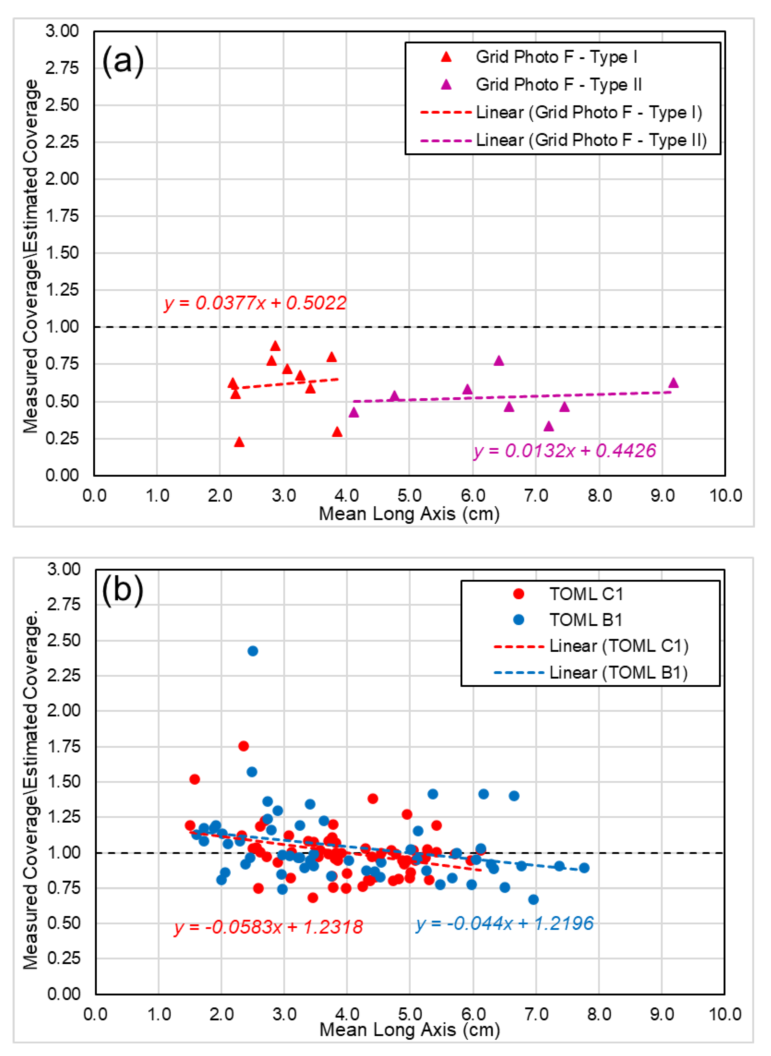
4.2.1. Prediction of Nodule Coverage: Idealized Nodules
4.2.2. Prediction Nodule Abundance I: Based on “Idealized Nodule” Model
4.2.3. Prediction Nodule Abundance II: With Empirical Long-Axis-Weight Relationship
4.2.4. Relation between Nodule Percentage Coverage and Abundance
- Equations (15) and (19) can be used independently to calculate the nodule percentage coverage and the abundance , respectively.
- If an estimation of the is already estimated (e.g., using digitization technique from seabed imagery), then Equation (28) or Equation (29) can be used to compute .
5. Test of Hypotheses of the Idealized Nodule Model
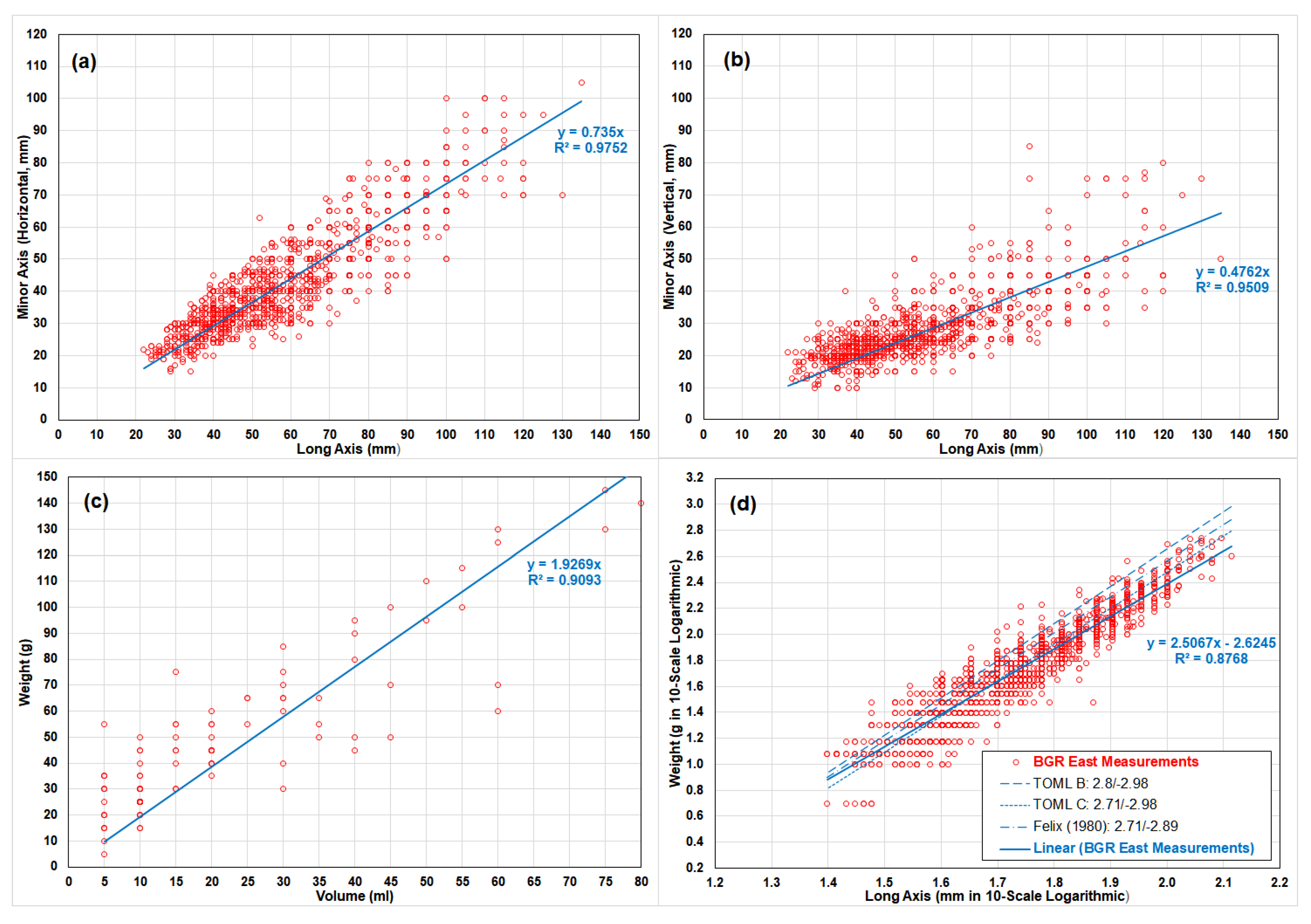
5.1. Test of Hypothese 1 and 2: Linear Regression Analyses on Nodule Dimensions and Weights
- Case 1: Nodule long axis and its horizontal minor axis;
- Case 2: Nodule long axis and its vertical minor axis;
- Case 3: Nodule weight and its volume; and
- Case 4: Nodule long axis and its weight.
5.2. Test of Hypothses 3: Goodness-of-Fit Test of Generalized Rayleigh Distribution for Nodule Long Axes
5.3. Comments on the Level of Support
6. Numerical Results of Nodule Resource Prediction Using the New Empirical Method
6.1. Sample Datasets
- 1.
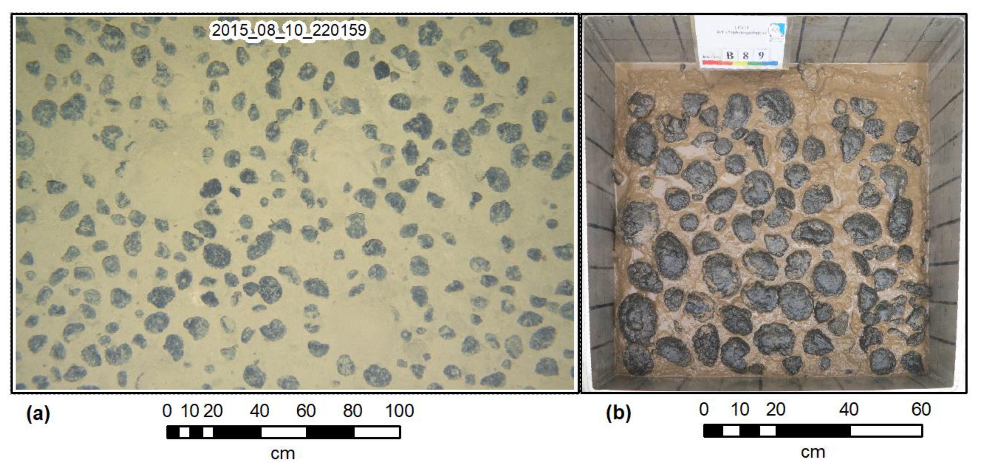
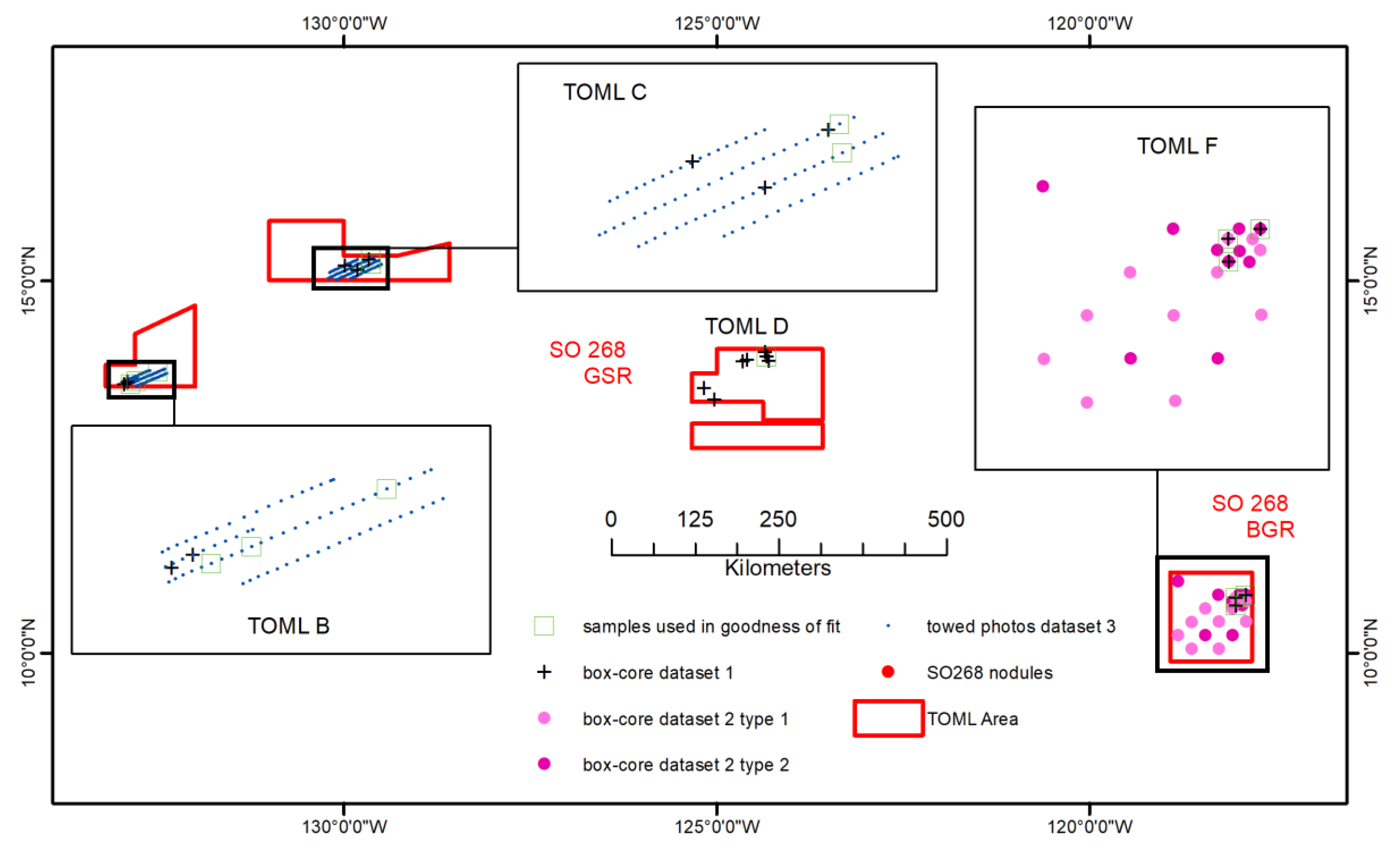
- Dataset 1: regional scale box-core sample dataset (physical weights). This involves four TOML exploration contract areas (TOML B, C, D, F; Figure 9) spanning some 2000 km of longitude and 700 km of latitude. The dataset thus allows for examination of a general relationship.
- 2.
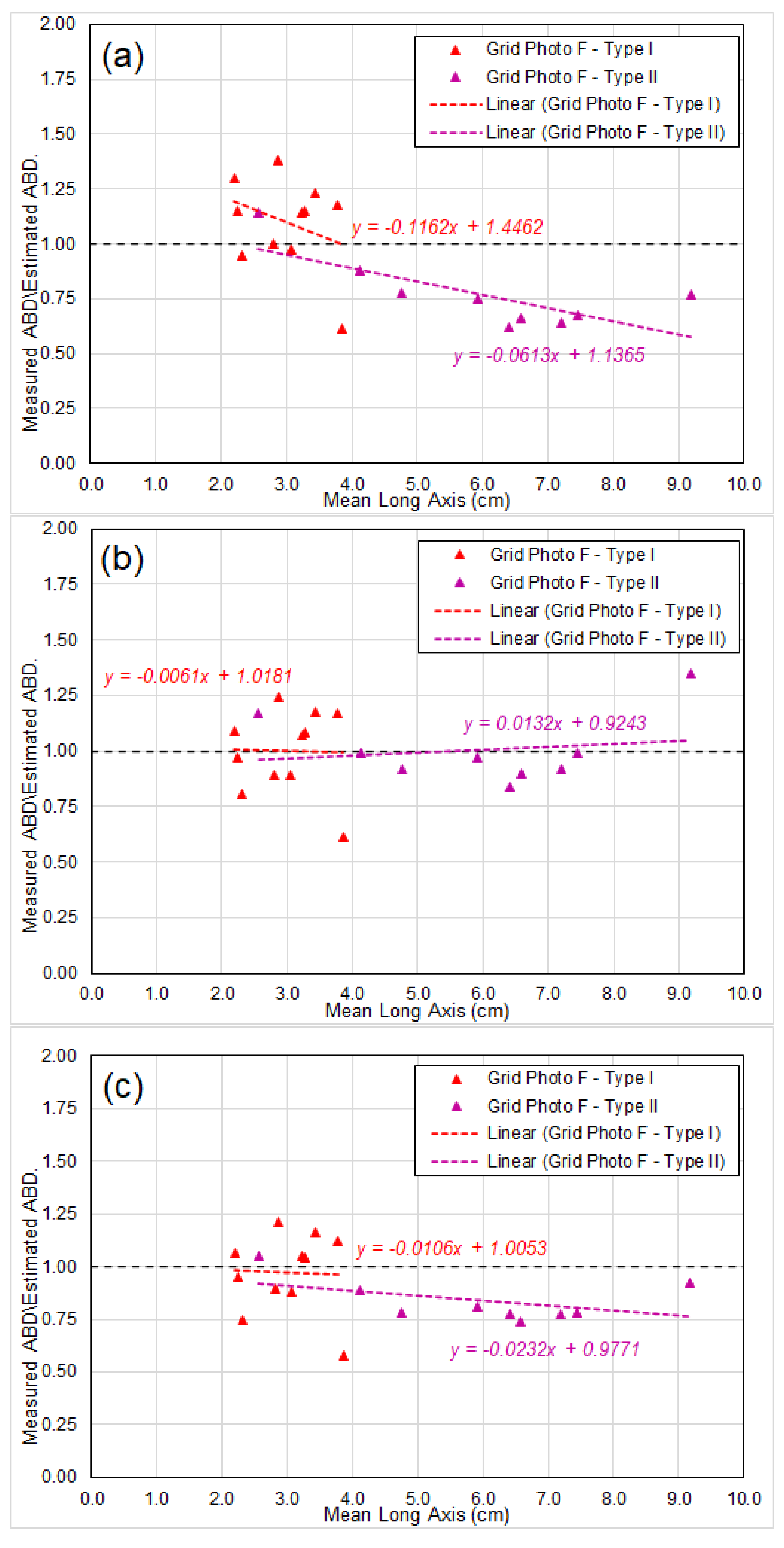
- Dataset 2: local scale box-core sample dataset (physical weight) of two distinct facies types but only within the TOML F area (~200 × 200 km). Type 1 nodules are smaller and often densely packed, type 2 nodules are significantly larger and more variable (cf. [5]). The dataset thus allows for differences in nodule types from an area where the distinction between type is simple and straightforward.
- 3.
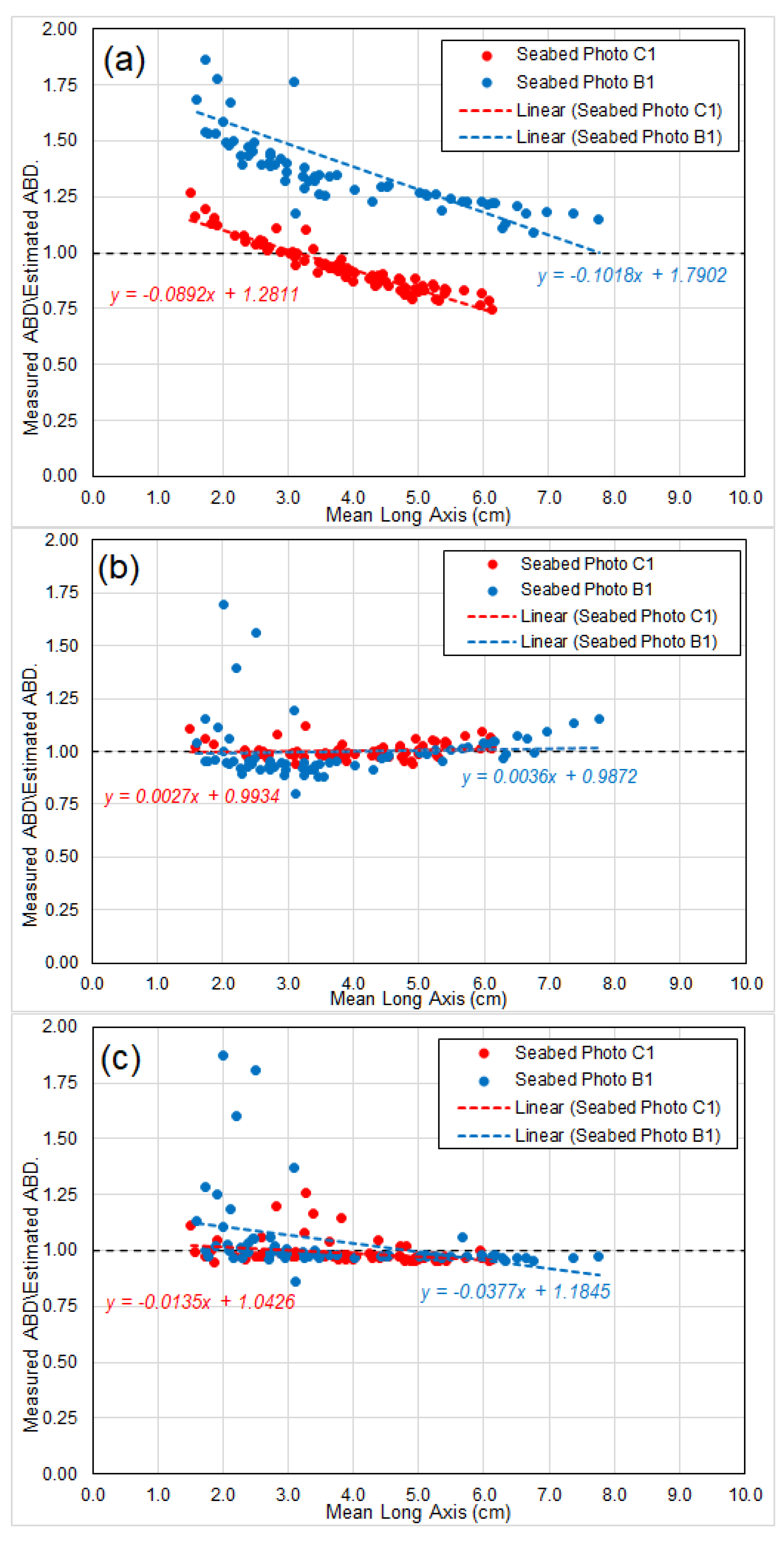
- Dataset 3: two local scale towed photo sample datasets (long-axis abundance estimate) between the TOML B and C areas (~300 km apart). The dataset is limited in that actual nodule weights cannot be compared, but it allows for larger datasets from two distinctly different areas to be compared.
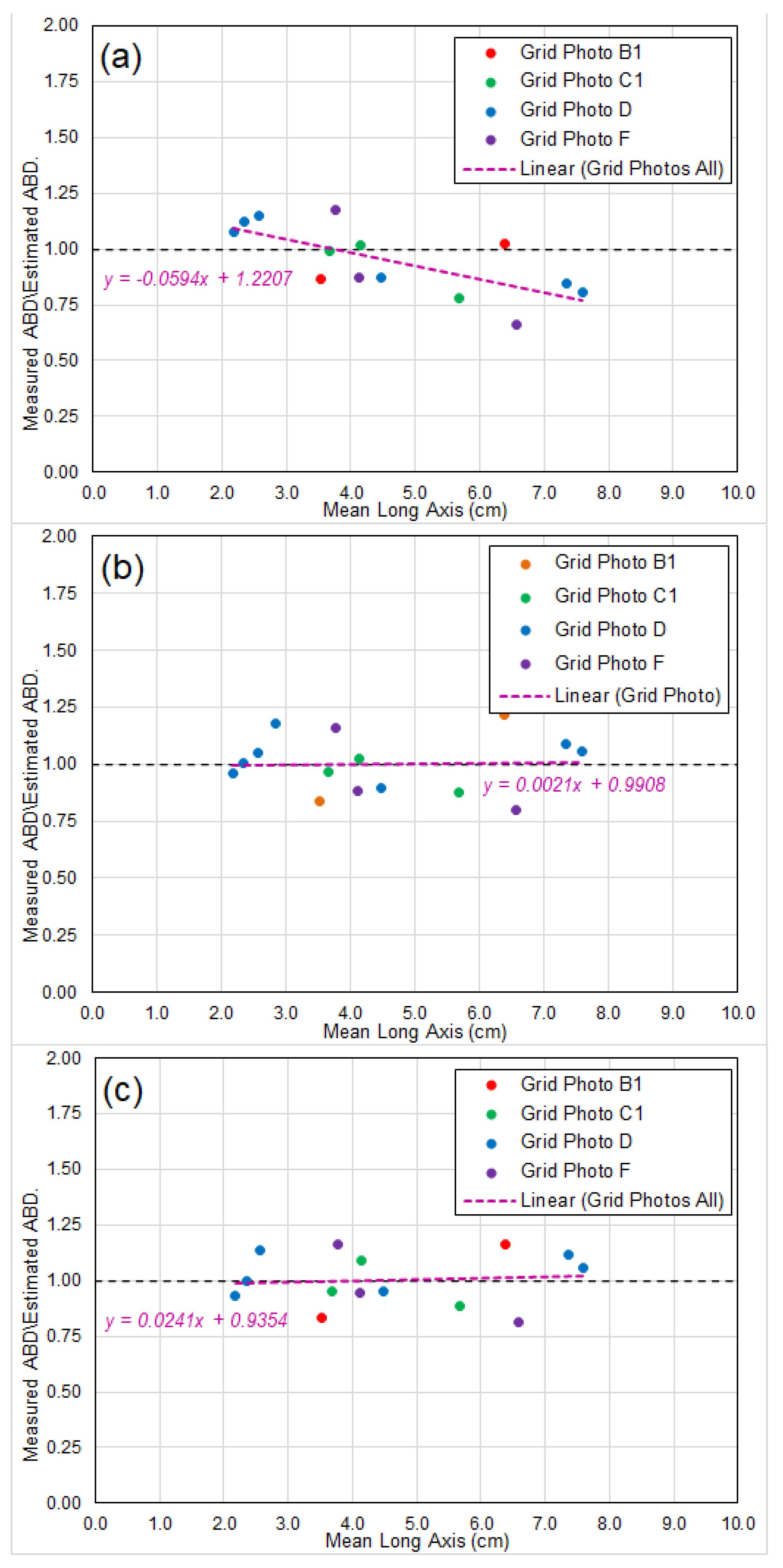
6.2. Prediction of Abundance of Seabed Nodules
- Chart (a) showing ratios based on abundance calculated directly by the empirical formula Equation (19), which is strictly based on the three hypotheses for idealized nodule model in Section 2. The axis ratios and used in the formula are extracted from the analyses of BGR East and GSR Central data (Table 1 in Section 5.1);
- Chart (b) showing the ratios in Chart (a) corrected by a “linear adjustment”. Each individual ratio in Chart (a) is factored/divided by the result of linear regression of the ratios, and the corrected results are shown in Chart (b); and
- Chart (c) showing ratios based on abundance calculated by the empirical formula Equation (19), incorporating the long-axis-weight relationship observed by several researchers (e.g., Felix [13]), which indicates the nodule weight is coorelated to the 2.7–2.8th power of its long-axis (noting for “idealized nodule”, it is the 3rd power).
7. Conclusions
- There is statistically significant evidence that the forms of CCZ polymetallic nodules resemble an “idealized nodule” model based on three hypotheses: (1) broadly ellipsoidal shape, (2) similar forms between nodules in a given area and (3) the nodule long axes follow a two-parameter Generalized Rayleigh Distribution (GRD). These three hypotheses were tested using field measurements from available nodule samples collected from CCZ. Numerical evidence supports the three hypotheses, possibly due to the relatively stable seabed environment and the long growth period of the nodules removing short-term transient effects.
- The distribution of nodules sizes and associated parameters can be estimated using empirical formulae. Specifically, explicit empirical formulae have been derived for direct calculation of GRD parameter α and β (Equation (11)), for percentage coverage CN (Equation (15)), and for abundance AN (Equation (19) or Equation (25)). These formulas are found to be sufficiently accurate for mineral resource estimation and are much easier to use than the traditional analytical methods for GRD.
- The direct application of the formula for AN does display a slight bias of over-estimating the abundance for larger nodules. However, unbiased accurate prediction of nodule abundance can be achieved by applying either a “linear adjustment” or a long-axis-weight relationship.
- For two of the TOML areas the new empirical method provides close agreement but from the third area there is a consistent offset. This may be related to the degree of clay-ooze sediment cover in that third area. Analyses of samples from other regions will be needed to better understand the generality of the empirical model and its derived formulae. Such analysis is needed in any event to calibrate the model in other areas.
- The new empirical method with derived explicit formulae has shown the potential of achieving more accurate mineral resource estimation with reduced sample numbers and sizes. The new understanding of the nodule size distribution can likely also improve the efficiency of design and configuration of mining equipment with limitations regarding particle size.
Author Contributions
Funding
Institutional Review Board Statement
Informed Consent Statement
Data Availability Statement
Acknowledgments
Conflicts of Interest
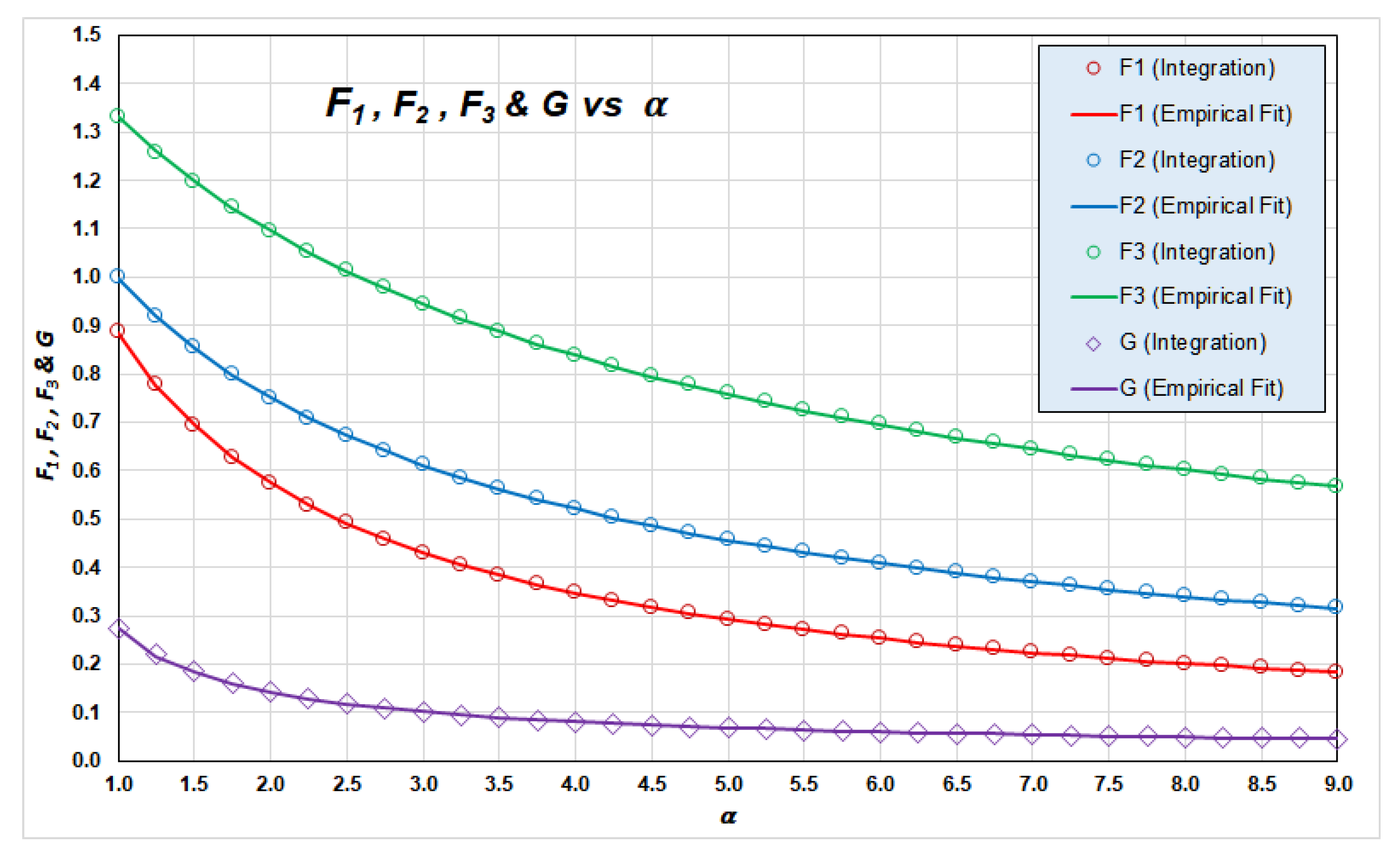
Appendix A. Functions , and
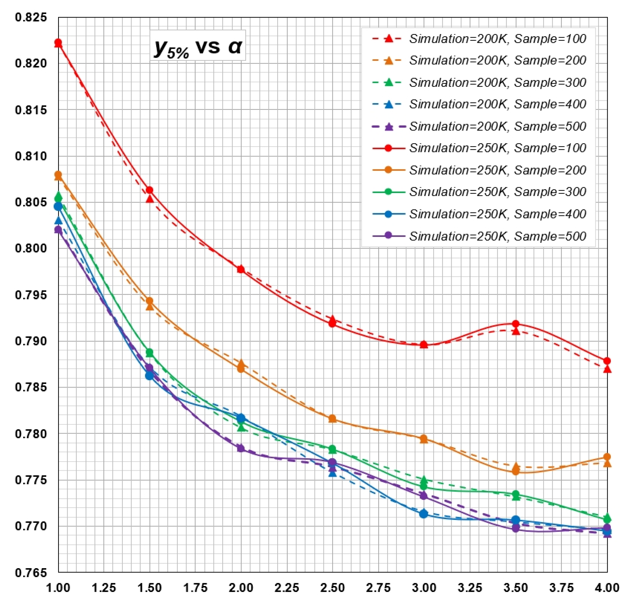
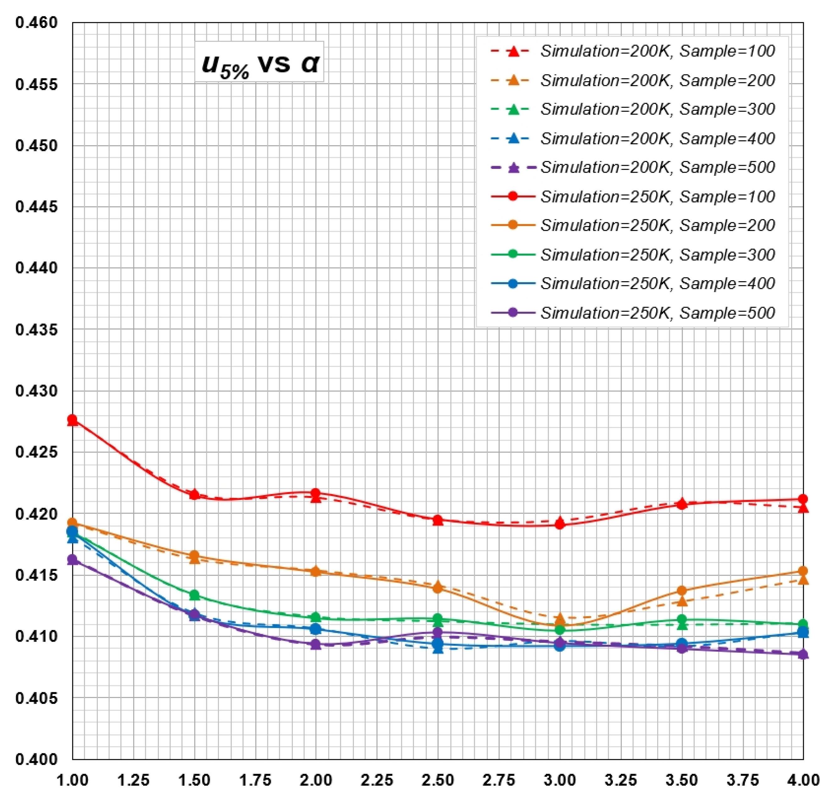
Appendix B. Computation of Critical Values for Goodness-of-Fit Test of Generalized Rayleigh Distribution by Monte Carlo Simulations
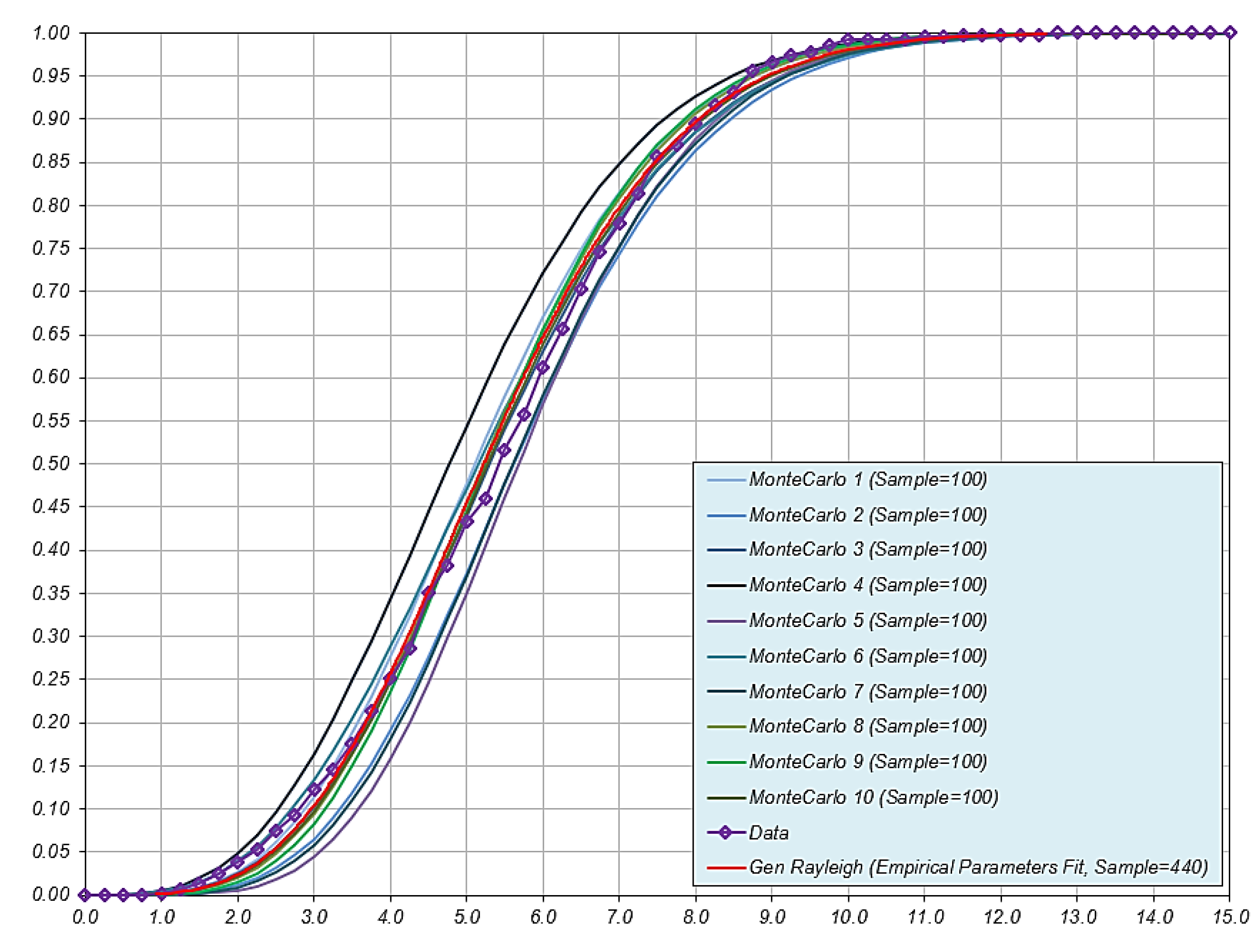
- A set of random numbers of size n is generated in the interval as values of cumulative distribution function (CDF). Equation (2) is used to back-calculate a sample of size n for given and .
- For a sample , Equations (5) and (6), based on MLE method, are solved iteratively to estimate parameters and .
- Parameters and are used in Equation (2) to calculate , with values in ascending order.
- Equation (7) is used to calculate test statistics and , using values of calculated in step 3.
- Steps 1. to 4. above are repeated to generate a sample for and .
- The percentiles of and are calculated as critical values. The th percentile is taken as the critical value for the level of significance of γ.

| Shape Parameter α | 1.0 | 1.5 | 2.0 | 2.5 | 3.0 | 3.5 | 4.0 | ||||||||||||||||
|---|---|---|---|---|---|---|---|---|---|---|---|---|---|---|---|---|---|---|---|---|---|---|---|
| Significance Level γ | 10% | 5% | 1% | 10% | 5% | 1% | 10% | 5% | 1% | 10% | 5% | 1% | 10% | 5% | 1% | 10% | 5% | 1% | 10% | 5% | 1% | ||
| Sample Size n | 100 | 0.66 | 0.79 | 1.10 | 0.65 | 0.78 | 1.08 | 0.64 | 0.77 | 1.07 | 0.64 | 0.76 | 1.06 | 0.64 | 0.76 | 1.05 | 0.64 | 0.76 | 1.05 | 0.64 | 0.76 | 1.05 | |
| 0.34 | 0.41 | 0.58 | 0.34 | 0.41 | 0.57 | 0.33 | 0.41 | 0.57 | 0.33 | 0.40 | 0.57 | 0.33 | 0.40 | 0.57 | 0.33 | 0.41 | 0.57 | 0.34 | 0.41 | 0.57 | |||
| 200 | 0.66 | 0.79 | 1.11 | 0.65 | 0.78 | 1.08 | 0.65 | 0.77 | 1.07 | 0.64 | 0.77 | 1.05 | 0.64 | 0.76 | 1.05 | 0.64 | 0.76 | 1.06 | 0.64 | 0.76 | 1.05 | ||
| 0.34 | 0.41 | 0.58 | 0.34 | 0.41 | 0.58 | 0.34 | 0.41 | 0.57 | 0.34 | 0.41 | 0.57 | 0.34 | 0.40 | 0.57 | 0.34 | 0.41 | 0.57 | 0.34 | 0.41 | 0.57 | |||
| 300 | 0.66 | 0.79 | 1.10 | 0.65 | 0.78 | 1.08 | 0.65 | 0.77 | 1.08 | 0.64 | 0.77 | 1.06 | 0.64 | 0.76 | 1.05 | 0.64 | 0.76 | 1.05 | 0.64 | 0.76 | 1.06 | ||
| 0.34 | 0.41 | 0.58 | 0.34 | 0.41 | 0.58 | 0.34 | 0.41 | 0.57 | 0.34 | 0.41 | 0.57 | 0.34 | 0.41 | 0.57 | 0.34 | 0.41 | 0.57 | 0.34 | 0.41 | 0.57 | |||
| 400 | 0.66 | 0.80 | 1.11 | 0.65 | 0.78 | 1.08 | 0.65 | 0.77 | 1.07 | 0.64 | 0.77 | 1.06 | 0.64 | 0.76 | 1.06 | 0.64 | 0.76 | 1.06 | 0.64 | 0.76 | 1.05 | ||
| 0.34 | 0.41 | 0.59 | 0.34 | 0.41 | 0.58 | 0.34 | 0.41 | 0.58 | 0.34 | 0.41 | 0.57 | 0.34 | 0.41 | 0.57 | 0.34 | 0.41 | 0.57 | 0.34 | 0.41 | 0.57 | |||
| 500 | 0.66 | 0.80 | 1.11 | 0.65 | 0.78 | 1.09 | 0.64 | 0.77 | 1.07 | 0.64 | 0.77 | 1.06 | 0.64 | 0.77 | 1.06 | 0.64 | 0.76 | 1.06 | 0.64 | 0.76 | 1.05 | ||
| 0.34 | 0.41 | 0.59 | 0.34 | 0.41 | 0.58 | 0.34 | 0.41 | 0.57 | 0.34 | 0.41 | 0.57 | 0.34 | 0.41 | 0.57 | 0.34 | 0.41 | 0.57 | 0.34 | 0.41 | 0.57 | |||


Appendix C. Determination of Minimal Sample Size for Estimation of Statistical Distribution Using Monte Carlo Simulations


References
- Haynes, B.W.; Law, S.L.; Barron, D.C.; Kramer, G.W.; Maeda, R.; Magyar, M. Pacific manganese nodules: Characterisation and processing. U.S. Geol. Surv. Bull 1985, 679, 44. [Google Scholar]
- International Seabed Authority. A Geological Model of Polymetallic Nodule Deposits in the Clarion-Clipperton Fracture Zone; International Seabed Authority: Kingston, Jamaica, 2010. [Google Scholar]
- Fouquet, Y.; Depauw, G. GEMONOD Polymetallic Nodules Resource Classification. In Proceedings of the Workshop on Polymetallic Nodule Resources Classification, Goa, India, 13–17 October 2014; International Seabed Authority: Kingston, Jamaica, 2014. [Google Scholar]
- Lipton, I.; Nimmo, M.; Parianos, J. TOML Clarion Clipperton Zone Project, Pacific Ocean; AMC Consultants Pty Ltd.: Brisbane, Australia, 2016. [Google Scholar]
- Lipton, I.; Nimmo, M.; Stevenson, I. NORI Area D Clarion Clipperton Zone Mineral Resource Estimate-Update; AMC Consultants Pty Ltd.: Brisbane, Australia, 2021. [Google Scholar]
- Ruhlemann, C.; Kuhn, T.; Wiedicke, M.; Kasten, S.; Mewes, K.; Picard, A. Current Status of Manganese Nodule Exploration in the German Licence Area. In Proceedings of the Ninth (2011) ISOPE Ocean Mining Symposium, Maui, HI, USA, 19–24 June 2011; International Society of Offshore and Polar Engineers, Ed.; International Society of Offshore and Polar Engineers: Mountain View, CA, USA, 2011; pp. 19–24. [Google Scholar]
- Yuzhmorgeologia. The concept of the Russian exploration area polymetallic nodules resource and reserve categorization. In Proceedings of the Workshop on Polymetallic Nodule Resources Classification, Goa, India, 13–17 October 2014; International Seabed Authority: Kingston, Jamaica, 2014. [Google Scholar]
- Korea Institute of Ocean Science; Technology Status of Korea. Activities in Resource Assessment and Mining Technologies. In Proceedings of the Workshop on Polymetallic Nodule Resources Classification, Goa, India, 13–17 October 2014; International Seabed Authority: Kingston, Jamaica, 2014. [Google Scholar]
- Deep Ocean Resources Development Co Ltd. Polymetallic Nodule Resources Evaluation—How we are doing. In Proceedings of the Workshop on Polymetallic Nodule Resources Classification, Goa, India, 13–17 October 2014; International Seabed Authority: Kingston, Jamaica, 2014. [Google Scholar]
- Interoceanmetal Joint Organization. Activities of the IOM within the scope of geological exploration for polymetallic nodule resources. In Proceedings of the Workshop on Polymetallic Nodule Resources Classification, Goa, Indi, 13–17 October 2014; International Seabed Authority: Kingston, Jamaica, 2014. [Google Scholar]
- International Seabed Authority. Secretary General Annual Report; International Seabed Authority: Kingston, Jamaica, 2020. [Google Scholar]
- Kaufman, R. The Selection and Sizing of Tracts Comprisinq a Manganese Nodule Ore Body. In Proceedings of the All Days, Houston, TX, USA, 5–7 May 1974. [Google Scholar]
- Felix, D. Some problems in making nodule abundance estimates from sea floor photographs. Mar. Min. 1980, 2, 293–302. [Google Scholar]
- Schoening, T.; Gazis, I.-Z. Sizes, Weights and Volumes of poly-Metallic Nodules from Box Cores Taken during SONNE Cruises SO268/1 and SO268/2. Available online: https://doi.pangaea.de/10.1594/PANGAEA.904962 (accessed on 9 February 2021).
- Ellefmo, S.L.; Kuhn, T. Application of Soft Data in Nodule Resource Estimation. Nat. Resour. Res. 2020, 30, 1069–1091. [Google Scholar] [CrossRef]
- Mucha, J.; Wasilewska-Błaszczyk, M. Estimation Accuracy and Classification of Polymetallic Nodule Resources Based on Classical Sampling Supported by Seafloor Photography (Pacific Ocean, Clarion-Clipperton Fracture Zone, IOM Area). Minerals 2020, 10, 263. [Google Scholar] [CrossRef]
- Parianos, J.; Lipton, I.; Nimmo, M. Aspects of Estimation and Reporting of Mineral Resources of Seabed Polymetallic Nodules: A Contemporaneous Case Study. Minerals 2021, 11, 200. [Google Scholar] [CrossRef]
- Sharma, R. Computation of Nodule Abundance from Seabed Photos. In Proceedings of the Offshore Technology Conference, Houston, TX, USA, 1–4 May 1989; Offshore Technology Conference: Houston, TX, USA, 1989. [Google Scholar]
- Park, S.-H.; Park, C.-W.; Kim, C.-W.; Kang, J.K.; Kim, K.-H. An Image Analysis Technique for Exploration of Manganese Nodules. Mar. Georesour. Geotechnol. 1999, 17, 371–386. [Google Scholar] [CrossRef]
- Longuet-Higgins, M.S. On the statistical distribution of the heights of sea waves. J. Mar. Res. 1952, 11, 245–266. [Google Scholar]
- Abd-Elfattah, A.M. Goodness of fit test for the generalized Rayleigh distribution with unknown parameters. J. Stat. Comput. Simul. 2011, 81, 357–366. [Google Scholar] [CrossRef]
- Savitzky, A.; Golay, M.J.E. Smoothing and Differentiation of Data by Simplified Least Squares Procedures. Anal. Chem. 1964, 36, 1627–1639. [Google Scholar] [CrossRef]


| Case | Regression Parameters | Regions | Sample Size | Estimated Slope | Estimated Intercept | Coefficient of Determination (R2) | |
|---|---|---|---|---|---|---|---|
| 1 | Minor Axis Y (Horizontal, mm) | Long Axis X (mm) | BGR East | 1376 | 0.7350 | 0 (Forced) | 97.52% |
| GSR Central | 259 | 0.7618 | 97.63% | ||||
| 2 | Minor Axis Z (Vertical, mm) | Long Axis X (mm) | BGR East | 1376 | 0.4762 | 0 (Forced) | 95.09% |
| GSR Central | 259 | 0.5389 | 96.83% | ||||
| 3 | Weight (g) | Volume (cm3) | BGR East | 99 | 1.9269 | 0 (Forced) | 90.93% |
| GSR Central | No Data | / | / | / | |||
| 4 | Weight (Logarithmic, g) | Long Axis X (Logarithmic, mm) | BGR East | 1376 | 2.5067 | −2.6245 | 87.68% |
| GSR Central | 259 | 2.7210 | −2.9439 | 93.13% | |||
| No | Sample ID | TOML Area | Type | Sample Size | Mean | Standard Deviation |
|---|---|---|---|---|---|---|
| 1 | 2015_08_10_172643 | B | Towed Photo | 336 | 3.091 | 2.512 |
| 2 | 2015_08_10_220159 | B | Towed Photo | 153 | 7.767 | 2.387 |
| 3 | 2015_08_11_121357 | B | Towed Photo | 403 | 5.978 | 1.732 |
| 4 | 2015_08_29_131349 | C | Towed Photo | 440 | 5.425 | 1.995 |
| 5 | 2015_09_02_185307 | C | Towed Photo | 113 | 3.827 | 1.270 |
| 6 | CCZ15-B51 | D | Washed Sample | 67 | 7.486 | 2.404 |
| 7 | CCZ15-B102 | F | Washed Sample | 278 | 4.318 | 1.705 |
| 8 | CCZ15-B106 | F | Washed Sample | 559 | 3.681 | 1.298 |
| 9 | CCZ15-B110 | F | Washed Sample | 135 | 6.910 | 2.602 |
| No | Sample ID | α | β | Conclusions | ||||
|---|---|---|---|---|---|---|---|---|
| 1 | 2015_08_10_172643 | 0.623 | 0.211 | 9.957 | 0.833 | 5.436 | 0.43 | Not Generalized Rayleigh |
| 2 | 2015_08_10_220159 | 2.714 | 0.162 | 0.66 | 0.784 | 0.257 | 0.414 | Generalized Rayleigh Dist. at 5% Level of Significance |
| 3 | 2015_08_11_121357 | 3.598 | 0.226 | 0.69 | 0.770 | 0.226 | 0.410 | |
| 4 | 2015_08_29_131349 | 1.965 | 0.210 | 0.541 | 0.777 | 0.305 | 0.408 | |
| 5 | 2015_09_02_185307 | 2.690 | 0.327 | 0.159 | 0.789 | 0.076 | 0.419 | |
| 6 | CCZ15-B51 | 1.701 | 0.144 | 0.376 | 0.804 | 0.200 | 0.423 | |
| 7 | CCZ15-B102 | 1.396 | 0.243 | 1.435 | 0.790 | 0.605 | 0.412 | Not Generalized Rayleigh |
| 8 | CCZ15-B106 | 2.410 | 0.321 | 0.738 | 0.778 | 0.314 | 0.410 | Generalized Rayleigh Dist. at 5% Level of Significance |
| 9 | CCZ15-B110 | 1.890 | 0.171 | 0.361 | 0.791 | 0.192 | 0.418 |
| Data-Set | TOML Areas | Number of Samples | Comparative Data Type | Range of Measured Abundances | Range of Mean Long Axes * | Range of Coefficient of Variation * |
|---|---|---|---|---|---|---|
| 1 | B, C, D, F | 2, 3, 7, 3 | Washed sample weights | 3.2 to 25.7 kg/m2 | 2.2 to 7.6 cm | 0.23 to 0.86 |
| 2 | F | 11 for Type 1 9 for Type 2 | Washed sample weights | 1.2 to 21.3 3.3 to 29.1 | 2.2 to 3.9 2.6 to 9.2 | 0.28 to 0.45 0.28 to 0.72 |
| 3 | B C | 68 85 | Long axis estimates on individual nodule images | 0.03 to 31 0.01 to 18 | 1.6 to 7.8 1.5 to 6.1 | 0.24 to 0.96 0.25 to 0.83 |
Publisher’s Note: MDPI stays neutral with regard to jurisdictional claims in published maps and institutional affiliations. |
© 2021 by the authors. Licensee MDPI, Basel, Switzerland. This article is an open access article distributed under the terms and conditions of the Creative Commons Attribution (CC BY) license (https://creativecommons.org/licenses/by/4.0/).
Share and Cite
Yu, G.; Parianos, J. Empirical Application of Generalized Rayleigh Distribution for Mineral Resource Estimation of Seabed Polymetallic Nodules. Minerals 2021, 11, 449. https://doi.org/10.3390/min11050449
Yu G, Parianos J. Empirical Application of Generalized Rayleigh Distribution for Mineral Resource Estimation of Seabed Polymetallic Nodules. Minerals. 2021; 11(5):449. https://doi.org/10.3390/min11050449
Chicago/Turabian StyleYu, Gordon, and John Parianos. 2021. "Empirical Application of Generalized Rayleigh Distribution for Mineral Resource Estimation of Seabed Polymetallic Nodules" Minerals 11, no. 5: 449. https://doi.org/10.3390/min11050449
APA StyleYu, G., & Parianos, J. (2021). Empirical Application of Generalized Rayleigh Distribution for Mineral Resource Estimation of Seabed Polymetallic Nodules. Minerals, 11(5), 449. https://doi.org/10.3390/min11050449