Author Contributions
A.S.C.: methodology, validation, formal analysis, investigation, writing—original draft preparation, and visualization; W.M.C.: conceptualization, methodology, validation, investigation, writing—review and editing, and resources; S.W.M.: conceptualization, project administrator, resources, writing—review and editing, supervision, and funding acquisition; R.J.B.: conceptualization, project administrator, writing—review and editing, investigation, and funding acquisition; M.H.: investigation, validation, writing—review and editing; C.K.: investigation, validation, writing—review and editing. All authors have read and agreed to the published version of the manuscript.
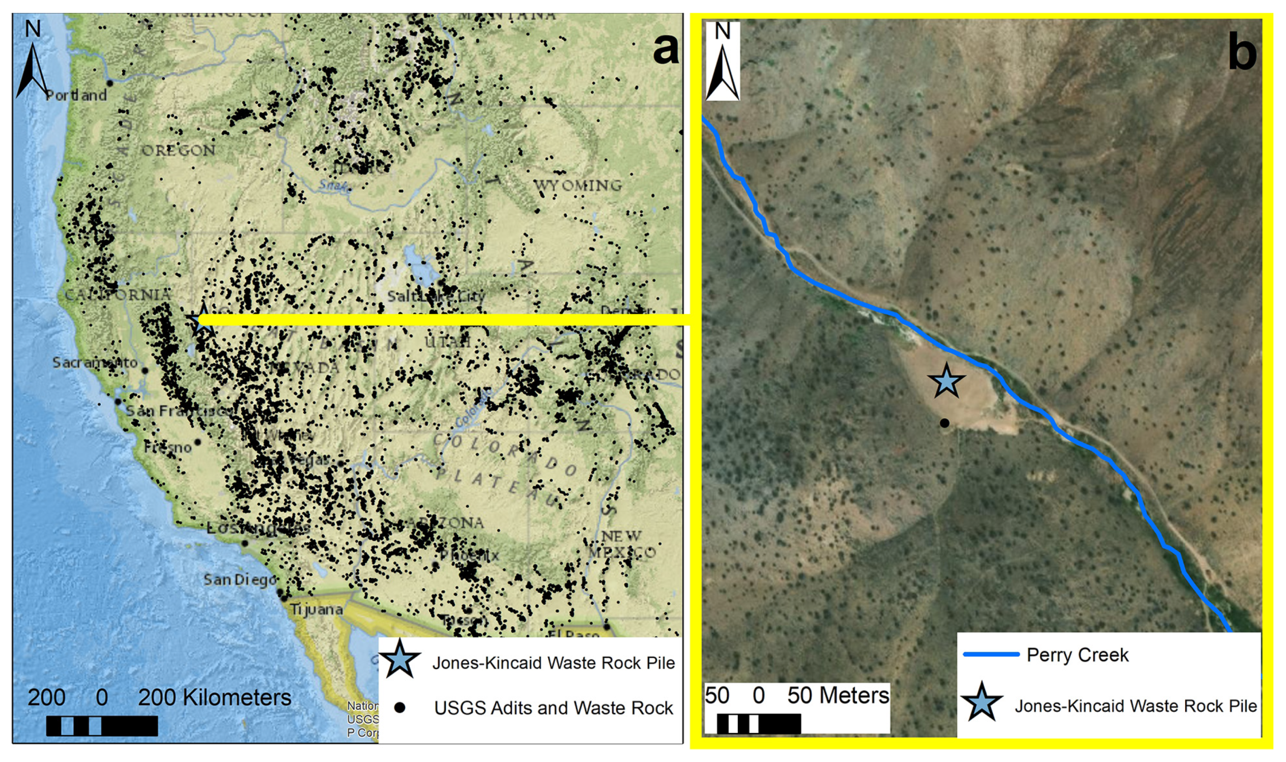
Figure 1.
(
a) Map of abandoned adits and waste rock piles, highlighitng the extent of inactive and active mine inventory in the Western U.S. [
19]; The Jones-Kincaid Waste Rock Pile in Perry Canyon, NV is indicated using a blue star. (
b) Jones-Kincaid Waste Rock study area and adjacent Perry Creek.
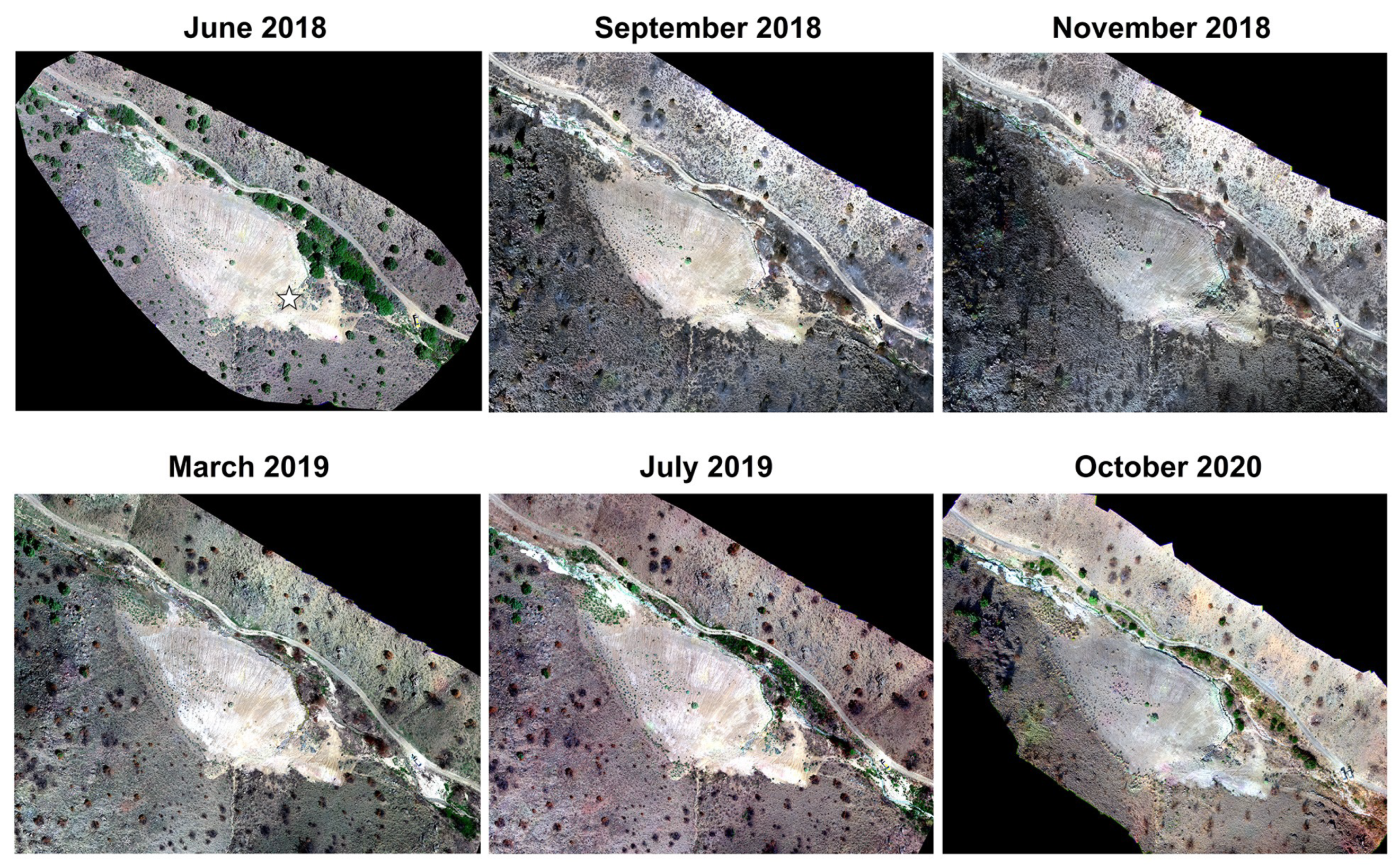
Figure 2.
Approximate true color reflectance maps using MicaSense channels centered on 668, 560, and 475 nm. North is up in each image. The scene is 240 m wide and 184 m tall. The adit drain is near the southeast corner of the waste rock pile, indicated with a star on the June 18 image.
Figure 2.
Approximate true color reflectance maps using MicaSense channels centered on 668, 560, and 475 nm. North is up in each image. The scene is 240 m wide and 184 m tall. The adit drain is near the southeast corner of the waste rock pile, indicated with a star on the June 18 image.
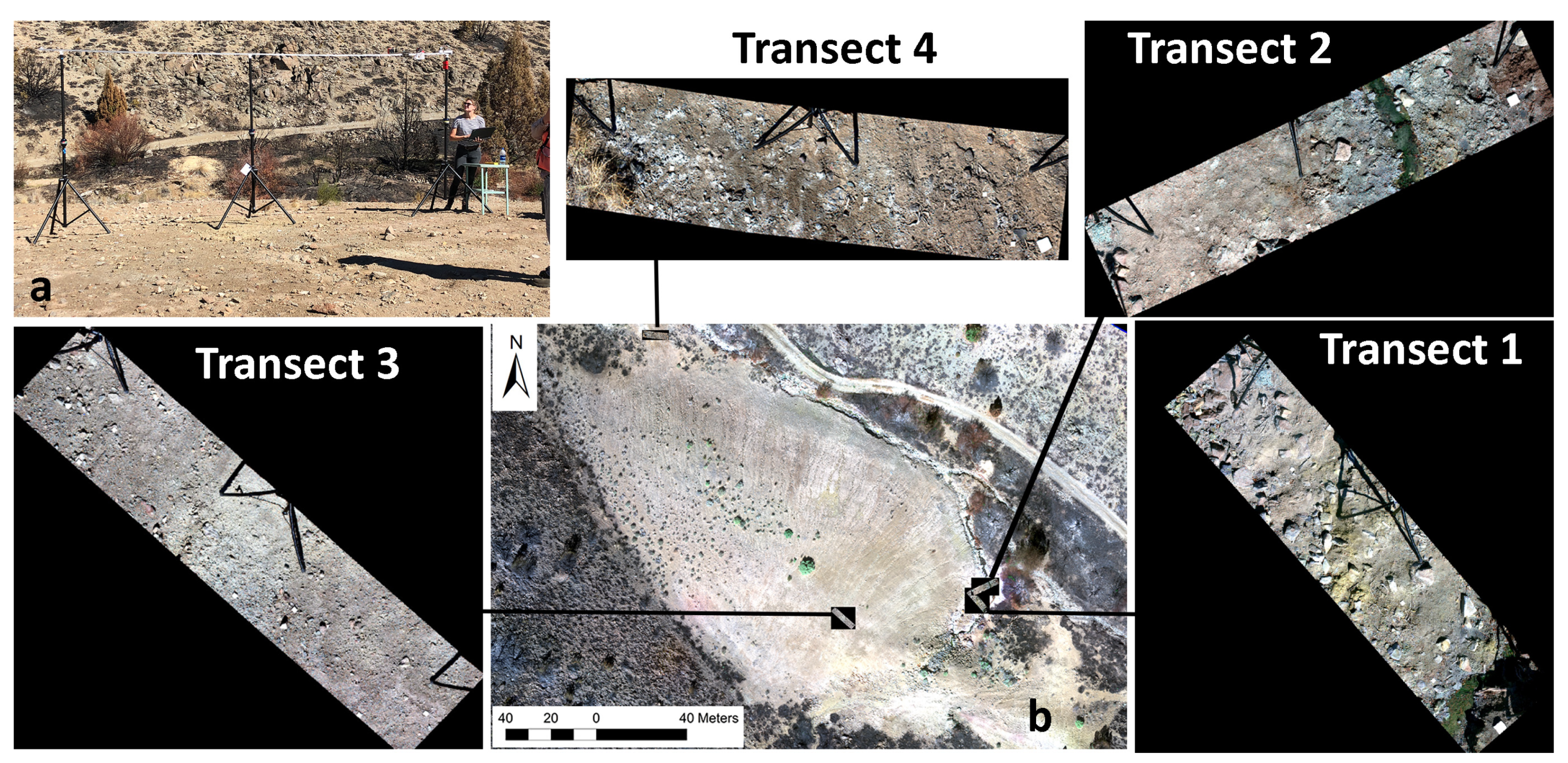
Figure 3.
(a) Custom-built motion-control system used for the Hyperspectral Surveys. (b) September 2018 UAS survey displaying locations for Transects 1–4 on the Jones-Kincaid waste cover, with zoomed images of Transects 1–4 using approximate true color RGB wavelengths (668 nm, 560 nm, 475 nm). Each Transect is 1.3 m wide, 5.5 m long.
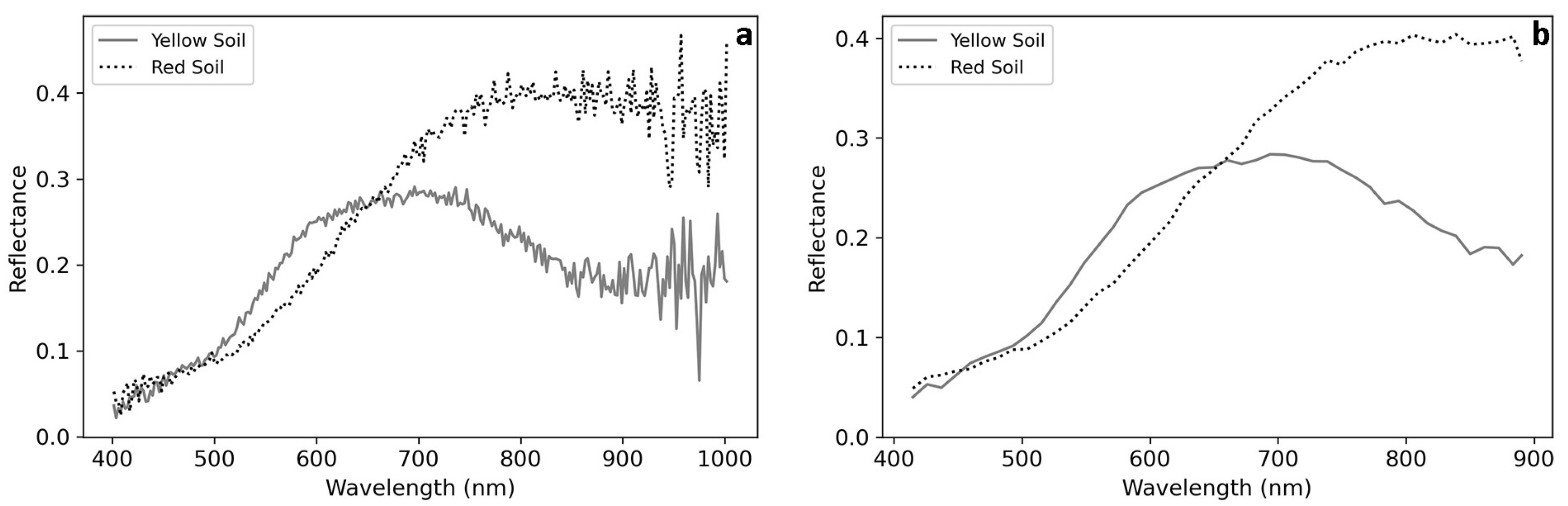
Figure 4.
(a) Raw spectral profiles of yellow and red soils on Transect 2 from the 271 band Nano VNIR Hyperspec camera. (b) Spectral profiles of the same yellow and red soils on Transect 2 post spectral averaging to 45 bands.
Figure 4.
(a) Raw spectral profiles of yellow and red soils on Transect 2 from the 271 band Nano VNIR Hyperspec camera. (b) Spectral profiles of the same yellow and red soils on Transect 2 post spectral averaging to 45 bands.
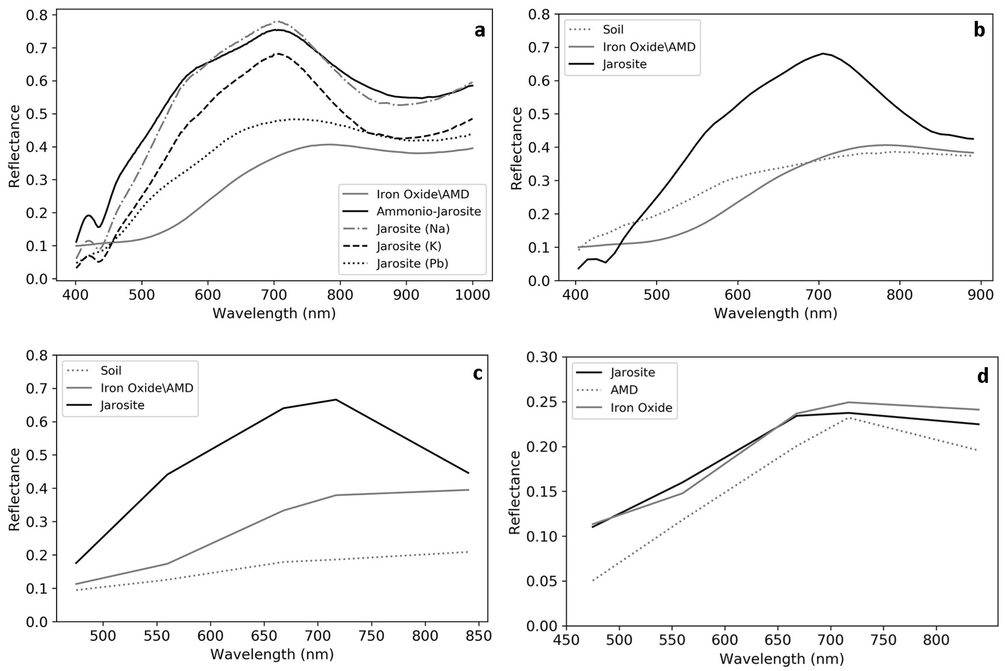
Figure 5.
(a) USGS Spectral Library Database (400–1000 nm), including 4 jarosite species and the iron oxide acid mine drainage assemblage, which is a mixture of secondary iron mineral precipitates coating a rock surface. (b) USGS Database re-sampled 45 bands from 450 to 850 nm. We combined the 4 jarosite species in to one class. (c) USGS Database re-sampled to 5 bands from 450 to 850 nm, with the 4 jarosite species combined in to one class. (d) Spectral profiles for iron oxide, AMD, and jarosite derived from ML classification polygons. These scene-derived endmembers show less pronounced shapes than the library minerals, but exhibit similar trends to the re-sampled USGS data in (c). Iron oxide has an upturn and steep slope from 550 to 650 nm, while jarosite has a downturn from 700 to 850 nm. The shape of the AMD profile exhibits both trends.
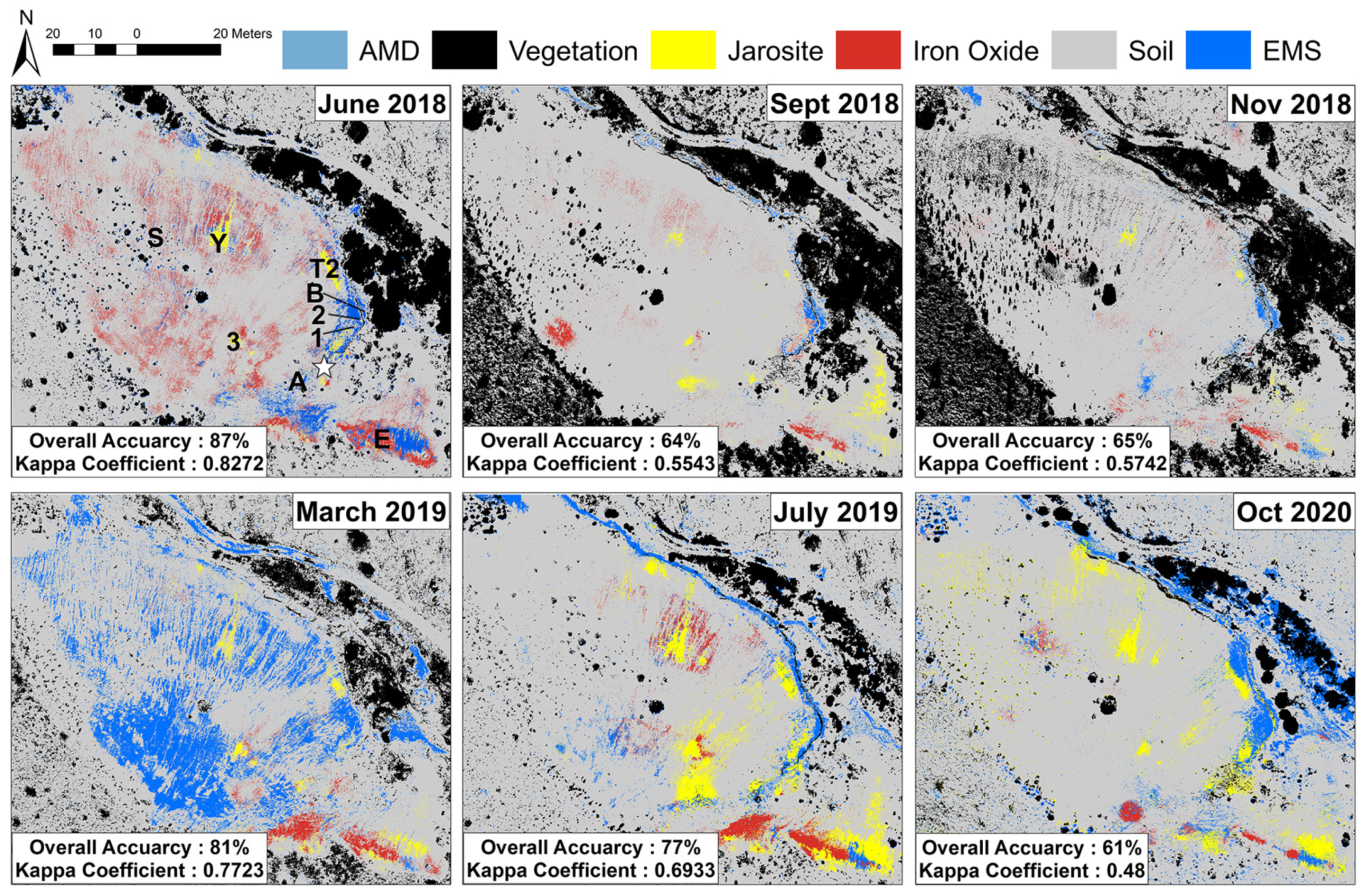
Figure 6.
Results of Maximum Likelihood Classification for each remotely piloted aerial system survey. Overall Accuracy for all six surveys is 72.5%, with a Kappa Coefficient of 0.6502. Locations for ground surveys are indicated on the June 2018 map for Y, T2, B, A, E, S, and Transects 1–3 (1,2,3), and the adit drain is indicated with a star. Each scene is 240 m wide and 184 m tall.
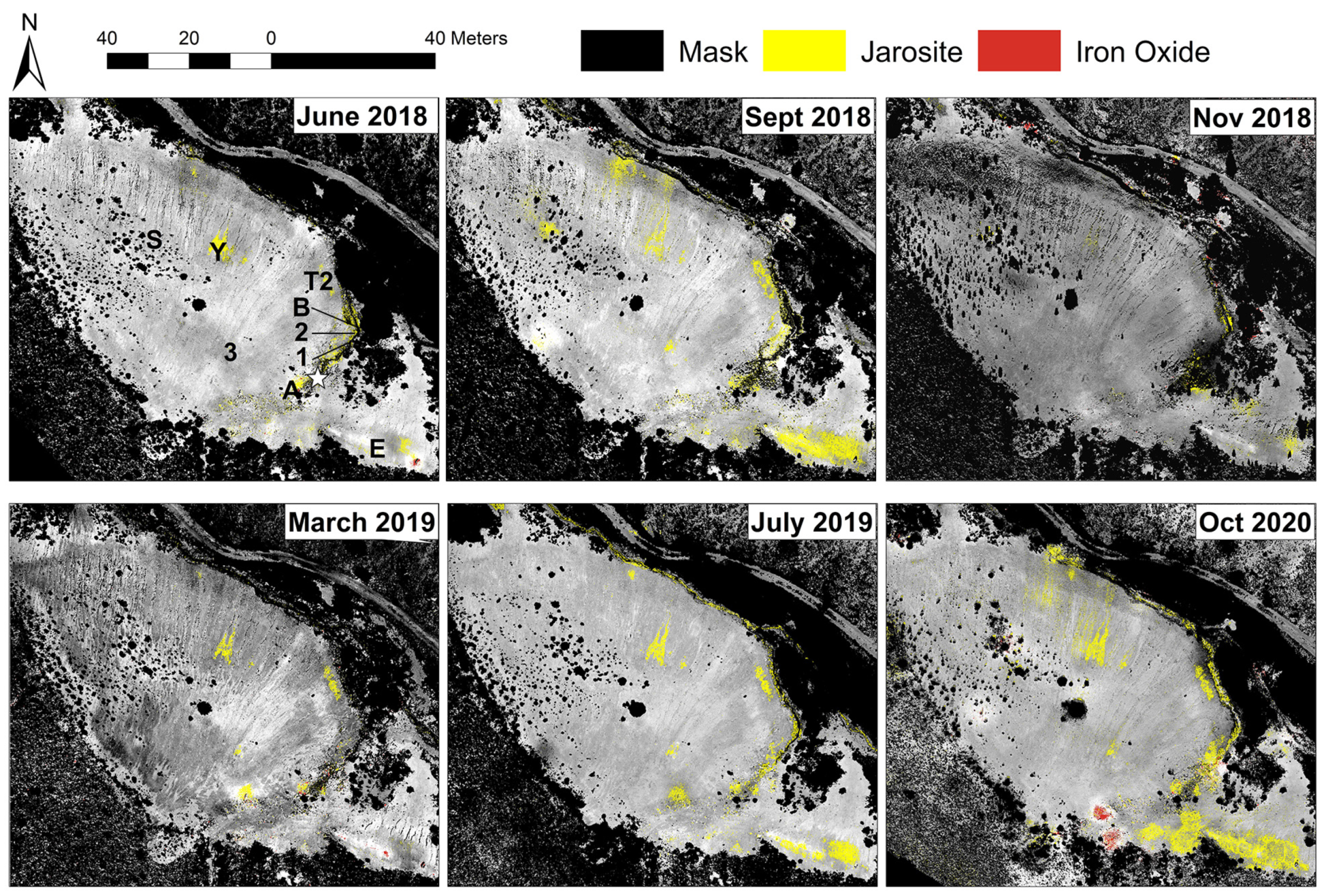
Figure 7.
Results of Spectral Angle Mapper Classification for each remotely piloted aerial system survey. Overall Accuracy for all six surveys is 80%, with a Kappa Coefficient of 0.7104. Locations for ground surveys are indicated on the June 2018 map for Y, T2, B, A, E, S, and Transects 1–3 (1,2,3), and the adit drain is indicated with a star. Each scene is 134 m wide and 118 m tall.
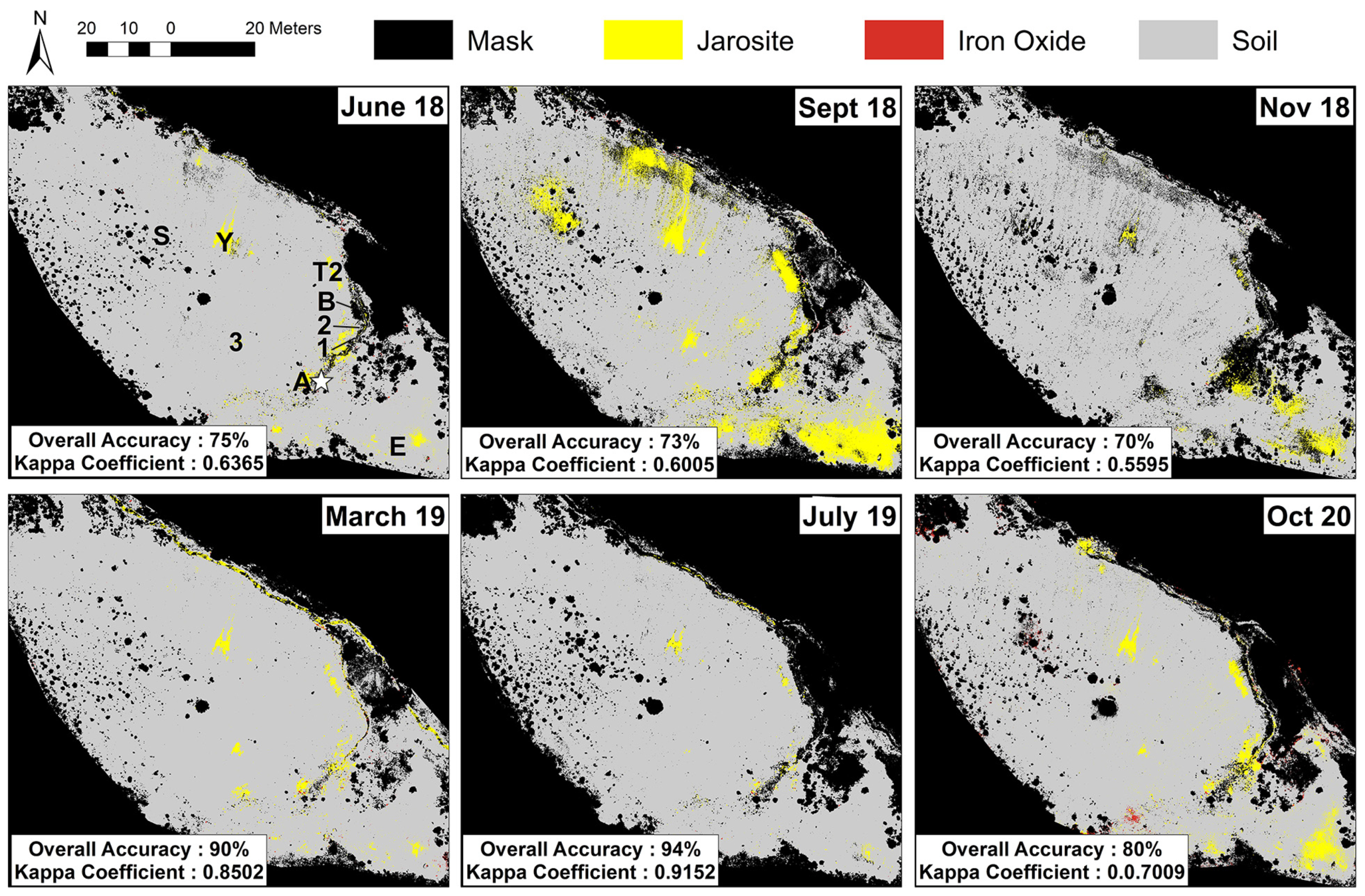
Figure 8.
Results of Band Math Ratios for each remotely piloted aerial system survey. Locations for ground surveys are indicated on the June 2018 map for Y, T2, B, A, E, S, and Transects 1–3 (1,2,3), and the adit drain is indicated with a star. Each scene is 134 m wide and 118 m tall.
Figure 8.
Results of Band Math Ratios for each remotely piloted aerial system survey. Locations for ground surveys are indicated on the June 2018 map for Y, T2, B, A, E, S, and Transects 1–3 (1,2,3), and the adit drain is indicated with a star. Each scene is 134 m wide and 118 m tall.
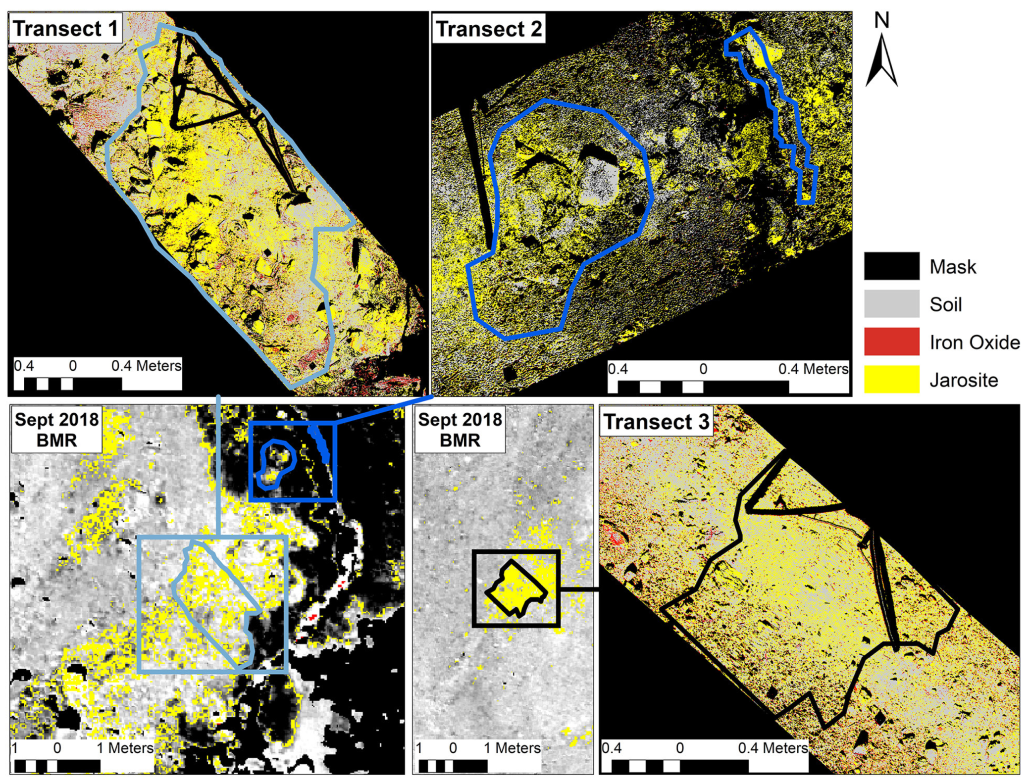
Figure 9.
Validation of jarosite in the September 2018 Band Math Ratio classification in Transects 1–3. Jarosite is outlined in black on Transect 3, in dark blue on Transect 2, and in light blue on Transect 1. Each transect location and mapped jarosite area is highlighted on the corresponding September 2018 band math ratio map as called out by color bars linking the band math ratio image to the hyperspectral data.
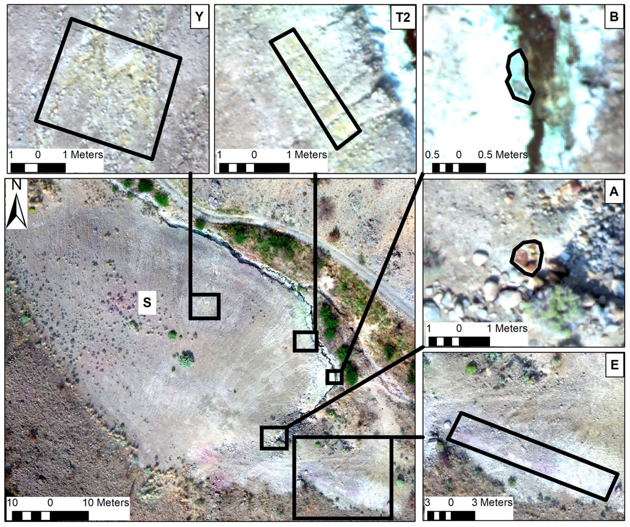
Figure 10.
Locations for the field spectral measurements in October 2020. Y, T2, B, A, E, locations are represented by boxes on the October 2020 reflectance map, and the zoomed in images indicate the exact locations for spectra shown in
Figure 11. S is the location of the second trench site.
Figure 10.
Locations for the field spectral measurements in October 2020. Y, T2, B, A, E, locations are represented by boxes on the October 2020 reflectance map, and the zoomed in images indicate the exact locations for spectra shown in
Figure 11. S is the location of the second trench site.
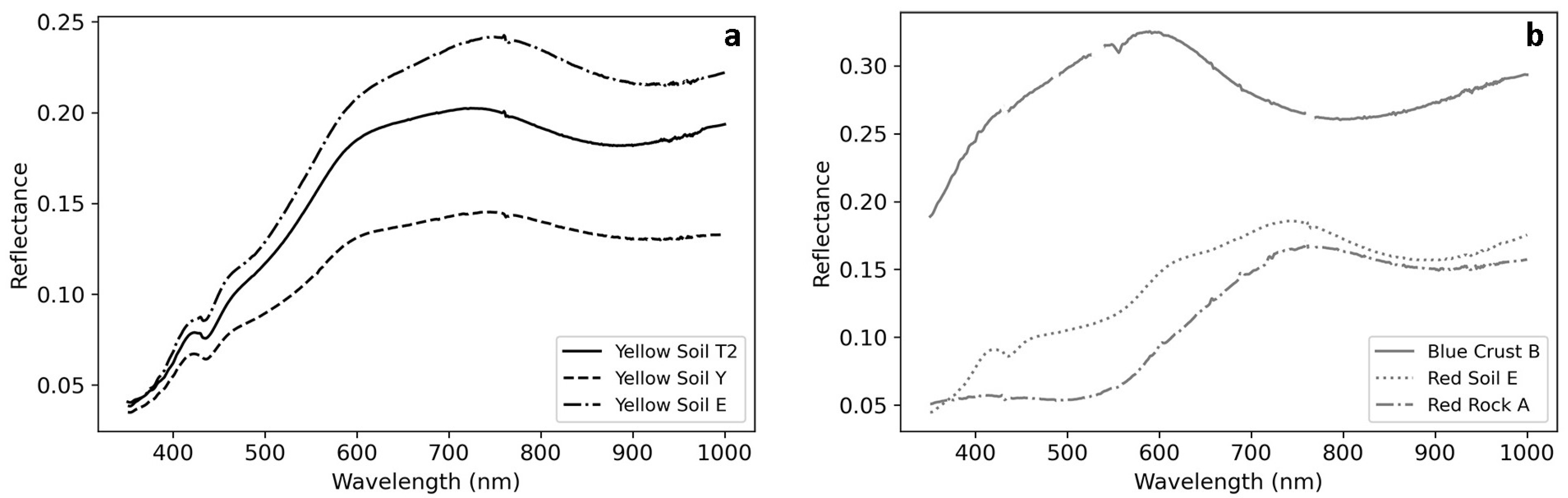
Figure 11.
Spectral profile results of the October 2020 ground survey. (
a) Yellow soil spectral profiles at Y, T2, and E. (
b) Spectral profiles for EMS at B, and red soils at E and A. Each field spectroscopy sample was taken with the field portable remote sensing spectroradiometer. See
Figure 10 for locations.
Table 1.
Micasense 5-band multispectral sensor wavelengths.
Table 1.
Micasense 5-band multispectral sensor wavelengths.
| Spectral Bands | Wavelength (nm) | Bandwidth (nm) |
|---|
| Blue | 475 | 20 |
| Green | 560 | 20 |
| Red | 668 | 20 |
| Red Edge | 717 | 10 |
| Near-Infrared (NIR) | 850 | 40 |
Table 2.
Micasense 5-band multispectral sensor specifications.
Table 2.
Micasense 5-band multispectral sensor specifications.
| Sensor | Sensor Dimensions (mm) | Focal Length (mm) | Shutter Type |
|---|
| Micasense 5-Band Multispectral Sensor | 4.8 × 3.6 | 5.5 | Rolling |
Table 3.
Pix4D structure from motion processing details and results for the orthorectified reflectance maps.
Table 3.
Pix4D structure from motion processing details and results for the orthorectified reflectance maps.
| Survey Date | Area (km) | GSD (cm) | GCPs | MRE (Pixels) | Images Calibrated | Resolution (cm) |
|---|
| June 2018 | 0.025 | 2.9 | 8 | 0.024 | 1180/1180 | 2.9 |
| September 2018 | 0.2 | 3.63 | 15 | 0.038 | 5815/6238 | 3.63 |
| November 2018 | 0.149 | 3.79 | 11 | 0.029 | 6320/6785 | 3.79 |
| March 2019 | 0.19 | 3.5 | 14 | 0.125 | 7375/8060 | 3.5 |
| July 2019 | 0.159 | 3.78 | 14 | 0.361 | 5445/5690 | 3.78 |
| October 2020 | 0.031 | 2.71 | 8 | 0.161 | 3560/3651 | 2.71 |
Table 4.
Thresholds for Maximum Likelihood, where a - indicates that no threshold was used.
Table 4.
Thresholds for Maximum Likelihood, where a - indicates that no threshold was used.
| Class | J18 | S18 | N18 | M19 | J19 | O20 |
|---|
| Soil | - | - | - | - | - | - |
| Jarosite | 0.3 | 0.3 | 0.3 | - | - | - |
| Iron Oxides | 0.3 | 0.3 | 0.1 | 0.5 | - | - |
| AMD | - | - | - | 0.2 | - | - |
| EMS | - | - | - | - | - | - |


 ,
, 


