Detection of Rare Earth Elements in Minerals and Soils by Laser-Induced Breakdown Spectroscopy (LIBS) Using Interval PLS

Abstract

The numerous applications of rare earth elements (REE) has lead to a growing global demand and to the search for new REE deposits. One promising technique for exploration of these deposits is laser-induced breakdown spectroscopy (LIBS). Among a number of advantages of the technique is the possibility to perform on-site measurements without sample preparation. Since the exploration of a deposit is based on the analysis of various geological compartments of the surrounding area, REE-bearing rock and soil samples were analyzed in this work. The field samples are from three European REE deposits in Sweden and Norway. The focus is on the REE cerium, lanthanum, neodymium and yttrium. Two different approaches of data analysis were used for the evaluation. The first approach is univariate regression (UVR). While this approach was successful for the analysis of synthetic REE samples, the quantitative analysis of field samples from different sites was influenced by matrix effects. Principal component analysis (PCA) can be used to determine the origin of the samples from the three deposits. The second approach is based on multivariate regression methods, in particular interval PLS (iPLS) regression. In comparison to UVR, this method is better suited for the determination of REE contents in heterogeneous field samples.

1. Introduction

Rare earth elements (REE) are used in a wide range of modern technologies, which include, for instance, renewable energy technologies, communication technologies and petrochemistry [1,2,3]. Lanthanum and neodymium are relevant for electric mobility, for example, as well as for optimizing the material properties of steel alloys in conjunction with cerium. In the future, zirconium dioxide stabilized by yttrium will be applied as electrolyte material in fuel cells [2]. These diverse applications, especially in high-tech-industries, drive the global demand for REE. While in 2013 the need for REE in important future technologies accounted for about 30,900 t, studies predict an increasing demand of up to 70,900 t by 2035 [4]. Due to this increasing demand, REE are important resources [5]. Contrary to their name, they are widely distributed in the earth’s crust as trace elements. Due to the chemical similarity, elements of neighboring atomic numbers can substitute each other in the crystal structures of various minerals [1,6]. The most economically important REE-containing minerals are carbonates and phosphates, such as monazite, xenotime, bastnaesite or parisite. Within the minerals, the proportions of the various REE vary. Light REE (LREE), all elements from lanthanum to europium, predominate mainly in bastnaesite and monazite, whereas xenotime is a source of heavy REE (HREE), from gadolinium to lutetium and yttrium. This distribution depends on the deposit, its formation and type [1,3,6,7,8]. Although there is a large number of REE-rich minerals worldwide, mining is currently focused on a few deposits and minerals only. The mining of these resources is challenging, but the recycling of REE-containing products is also complicated [3]. Besides the aforementioned issues and the depletion of current deposits, bottlenecks in the availability of REE are expected in the future [9]. The world’s largest deposits are located in China. Currently, China is the world market leader in terms of REE production. Besides other Asian countries, there are several thousand tons of REE mined per year by Australia, the USA and Russia. To date, Europe has not mined any of the existing REE deposits. Economically relevant deposits can be found mainly in Scandinavia, especially in Sweden and Finland. These potential mining areas have elevated contents of REE and could cover the supply of Europe [3,6,10,11]. At the same time, the exploration of further REE deposits is growing in importance to ensure the supply in the future. Exploration requires fast, ecological and cost-efficient analytical methods, on the one hand to minimize the amount of sample material and, thus, the chemical and geological laboratory work, and to reduce the associated costs on the other hand [12]. The most common techniques to detect and analyze REE are inductively coupled plasma mass spectrometry (ICP-MS), inductively coupled plasma optical emission spectrometry (ICP-OES), X-ray fluorescence (XRF) and neutron activation analysis (NAA). However, most of these techniques are time-consuming and therefore expensive, for example due to sample preparation. In addition, almost all of these methods require prior sample collection for analysis in the laboratory [5,13,14,15]. Laser-induced breakdown spectroscopy (LIBS) is a method that allows rapid on-site analysis in real time. In addition, almost no sample preparation is required, as solid, liquid and gaseous samples can be analyzed in a wide variety of matrices. In comparison to XRF, all elements of the periodic table can be measured, including the lighter elements [5,12,13,16].

In LIBS, laser radiation is used to generate a plasma on the sample surface. The resulting emission allows the analysis of the investigated samples based on the spectral signatures of the characteristic elements [13]. Although the REE have numerous emission lines, the detection and analysis of the elements is difficult due to spectral interferences of the matrices and the low concentrations of the REE [5,16]. LIBS is often used for qualitative analysis of elements or for classification of minerals. Quantitative analysis is based on univariate and/or multivariate methods. Quantification by univariate regression (UVR) is often difficult, especially in heterogeneous materials, because numerous chemical and physical effects of the complex matrix can occur [12,17,18]. In contrast to univariate methods, the use of multivariate methods for quantification can remedy this situation. While univariate regression only includes individual peaks of the spectrum in the quantification, multivariate analysis techniques, such as partial least squares (PLS) regression, can include the entire spectrum or, through variable selection, just a partial spectrum. In the case of the application of the entire spectrum in PLS regression, the regression model contains noise and redundant information. This can have a negative impact on the prediction results. An alternative is to reduce the total spectrum to selected partial spectra, which contain the most important information by variable selection. This can potentially improve the predictive power of the model [19]. One such method is interval partial least squares (iPLS) regression. In this method the entire spectrum is divided into equally sized spectral intervals. From the resulting spectral sub-regions, the relevant information is provided and summarized, which facilitates focusing on important spectral regions and removing interference from other regions. PLS regression is performed on one spectral interval for each element [19,20]. The width of these intervals can vary. In the case of broad intervals, iPLS regression resembles a normal multivariate PLS regression. However, if the intervals become smaller, the iPLS regression could be considered an automated UVR. iPLS regression was first used in IR spectroscopy, but also finds application in other spectroscopic techniques, such as LIBS on soils [20,21].

The present work focuses on the utilization of LIBS for the exploration of new REE deposits. The aim is the quantitative screening of REE in minerals, rocks and soils in the surrounding area of a potential REE deposit using LIBS and univariate and multivariate iPLS regression. In this study, mineral, rocks and soil samples from the Scandinavian deposits Norra Kärr and Olserum in Sweden and Fen-Complex in Norway are investigated. Their elemental contents were determined by reference analysis (ICP-OES and XRF). The relatively small number of samples examined is a result of the high costs of sampling, transport and reference analysis. This problem accompanies geologists in their daily work and is used in this study to demonstrate the potential of our methods. In order to characterize the influence of matrix effects, synthetic REE samples produced from REE chloride salts in serpentinite and a model soil as well as the field samples are compared. All samples are analyzed with respect to the elements cerium (Ce), lanthanum (La), neodymium (Nd) and yttrium (Y). The results of the analysis with LIBS are evaluated with UVR and iPLS regression.

2. Materials and Methods

2.1. Samples and Reference Analysis

A total of 167 samples containing REE were analyzed. Of these, 122 were artificial samples (hereafter referred to as synthetic) and 45 were natural samples (hereafter referred to as field). In both cases, a further distinction was made between rock and soil samples. All samples were available as ground powders. The concentrations of REE in the synthetic samples are summarized in Table S1 in the Supplementary Materials. Table S2 contains the reference data of the composition of the field samples.

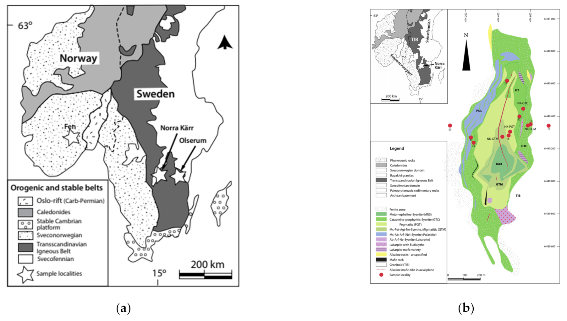
2.1.1. Geological Overview of Deposits

The field samples were collected at three different deposits in Sweden and Norway. 19 of these samples were taken in the Olserum-Jupval REE deposit in south east Sweden. Sampled outcrops are located ca. 7 km NW of Gambleby Västervik region (Figure 1a). REE-phosphates-rich dikes cross cut metasedimentary wall rocks (cordierite-bearing gneisses). The phosphates comprise monazite (LREE), xenotime (Y, HREE) and fluor-apatite (LREE). In addition, allanite (REE-silicate), and the REE carbonates bastnaesite and synchisite-Ce occur. The origin of the REE-deposit was studied in detail by Andersson et al. [22], Fullerton [23], Russel [24] and Gavelin [25]. REE-phospate-rich dikes of up to 2 m thickness occur near the contact to granitoids of the Transscandinavian Igneous Belt (ca. 1.85–1.65 Ga [26]) in the metasedimentary Västervik Formation. The samples are from two dikes located at a distance of ca. 150 m (from 57.94839N to 57.96364N, from 16.35213E to 16.32522E) [22,23,27].

The Norra-Kärr Complex is a small, magmatic intrusion with an “agpaitic composition”, i.e., (Na + K) > Al. The complex has an elliptical shape with a north–south extension of approx. 1300 m and an east–west extension of approx. 500 m (Figure 1a,b). The Norra Kärr Complex (ca. 1.5 Ga old [28]) intruded into igneous rocks of the Trans-Scandinavian Magmatic Belt (ca. 1.8–1.7 Ga [29]). It essentially consists of various types of nepheline syenites [26]. The original plutonic rocks show evidence of strong deformation and metamorphic overprint [30]. The tectonometamorphic overprinting is assigned to the Sveconorwegian orogeny (ca. 1048 Ga [31]). The rock sequence is known as a zirconium deposit due to the high abundance of Zr-rich minerals [26,32]. The major REE-bearing minerals are the silicates eudialyte, catapleiite and cerite. Eudialyte occurs as a REE-poor magmatic type and a HREE-rich secondary (metamorphic) type, which is the major REE-bearing phase. The analyzed rock and soil samples are from different parts of the intrusion, with slightly different compositions. The REE concentrations of the rocks are up to 1 wt.%. In addition, samples were taken from outside the intrusion as a reference (subsoil and topsoil Nr. 20). Another sample obtained to the east of the intrusion was contaminated by hydrothermal fluids, a so called fenitized rock. A total of 17 samples form Norra Kärr were examined [26,27,28,29,30,31,32].

The Fen Complex, located in the Telemark province of southern Norway, represents an early Cambrian magmatic intrusion complex. It is dominated by carbonatites, formed from carbonate melts [33,34,35,36,37]. The complex shows a surface outcrop of ca. 10 km². The previous carbonatitic melts intruded into Mesoproterozoic gneisses (Figure 1a). The carbonatites are interlayered by alkaline ultramafic silicate rocks, i.e., containing <40% SiO₂ [26]. All melts generated from a deeper mantle source. The carbonaceous intrusions modified the surrounding gneisses by CO₂-rich streams leading to alkaline metasomatic reactions. Therefore, the Fen Complex is the type locality of the “fenitisation-process”. The Fen Complex is known for its highly enriched thorium and rare earth concentrations [37]. The major REE-bearing minerals are monazite [(LREE,Th)PO₄], bastnaesite [(LREE)CO₃F] and parisite [Ca(LREE)₂(CO₃)₃F₂] [38]. Nine field samples for analyses of the Fen Complex were provided by the Federal Institute for Geosciences and Natural Resources (BGR) [38].

Reference analysis for the REE cerium, lanthanum and neodymium was carried out by inductively coupled plasma optical emission spectroscopy (ICP-OES) and X-ray fluorescence spectroscopy (XRF spectroscopy) for yttrium. The samples were available as ground powders. For LIBS measurement, all powders were pressed into pellets (TP 40, Herzog Maschinenfabrik, Osnabrück, Germany).

2.1.2. Preparation of the Synthetic Samples

The synthetic samples were prepared by standard addition. REE used as chloride hydrates (CeCl₃ · 7H₂O, LaCl₃ · 7H₂O, NdCl₃ · 6H₂O, YCl₃ · 6H₂O) were mixed with the respective matrices, soil and rock. For the samples in rock, a milled mixture of serpentinite and weathered crust was used. The matrix used in the soil-based samples is a soil containing loess from central Europe. The salts were obtained from Sigma Aldrich (St. Louis, MO, USA). The weighed rock samples were mixed with 3 wt.% distilled water, homogenized in a mill (MM 400, Retsch, Düsseldorf, Germany) and pressed into pellets (TP 40, Herzog Maschinenfabrik, Osnabrück, Germany). The soil samples were only homogenized and pressed into pellets. For one pellet, 3 g of sample is used. Pellets were prepared separately for each REE and concentration: 16 pellets for both Ce and Nd and 15 pellets for both La and Y were prepared, respectively (see Table S1 in the Supplementary Materials). Also, the pellets containing blank rock and soil were prepared for preliminary measurements but were not involved in iPLS regressions. The REE concentrations in the serpentinite and the soil were much less than 10 ppm.

2.2. Instrumental Set up of LIBS and Measurement Parameters

The samples were positioned on a rotating and linearly translating sample desk, resulting in a spiral-like measurement pattern. This ensured a fresh surface on the pellet for each ablation event. The light of the Nd:YAG laser (Bernoulli LIBS, Litron Lasers, Rugby, England, Great Britain, λ = 1064 nm, E = 20 mJ, repetition rate 10 Hz) was focused by a lens (focal length 50 mm) and created the plasma on the sample surface. Emissions were collected by a concave mirror (ME-OPT-0007, Andor Technology, Belfast, Northern Ireland, UK, focal length 52 mm, λ = 200–1100 nm) and focused on an optical fiber to guide the radiation to an echelle spectrometer (Aryelle Butterfly, LTB, Berlin, Germany). The two wavelength ranges (UV range: 190–330 nm, VIS range: 275–750 nm) of the spectrometer were measured separately with a resolution of 20–30 pm (delay time 2 µs). The spectrometer was equipped with an ICCD camera (iStar, AndorTechnology, Belfast, UK) as detector (gate width 10 µs). A total of about 230 spectra per sample were recorded in both the UV and VIS regions. For each spectrum, 10 single shots were accumulated.

2.3. Processing and Analysis of Data by Univariate and Multivariate Methods

Origin (OriginLab, Northampton, MA, USA) was used for univariate analysis. Matlab (Version 2019b, MathWorks, Natick, MA, USA) was used for the preprocessing and the multivariate methods PCA and iPLS regression.

Spectra were preprocessed by background correction and standard normal variate (SNV) normalization. A top-hat filter was used for the background correction. The utilized structure element length of 20 data points corresponds to a filter width of approximately 0.26 nm. The SNV normalization followed the background correction. For SNV normalization, the mean value of the entire spectrum was subtracted from the spectrum and the difference was divided by the standard deviation. After processing the data using background correction and SNV normalization, the 230 spectra were averaged so that one spectrum was finally obtained for each sample examined.

For the univariate regression, one element-specific peak was identified for each REE examined, and the peak area (A) was determined by integration of each of the 230 spectra and subsequent calculation mean and standard deviation. The peak area was plotted against the concentration. Principal component analysis was performed on the raw spectra of the field and synthetic samples.

For the iPLS regression, we used the iToolbox from Nørgaard [20]. The 230 spectra were averaged prior to iPLS and a separate iPLS was performed for each element, with the only input variables being the concentrations of the element in question. Cross validation was performed internally in the iPLS algorithm, as well as validation externally with test data excluded from the algorithm. The iPLS regression was based on variable selection in spectral intervals. The number of intervals was varied, with a maximum of 5000 intervals. Interval separation was performed on raw wavelength data. Due to the way echelle data is transformed from the 2D to the (standard) 1D representation, this resulted in intervals with different spectral widths (but constant numbers of sample points). The exact number of intervals and the number of components were determined individually for each sample (Tables 4 and 5) by systematic variation of the interval length. The interval number that resulted in an interval with the smallest RMSE was selected. The PLS regression was performed at this interval. Validation of the iPLS regression results was performed by 5-fold cross-validation with systematic exclusion.

3. Results

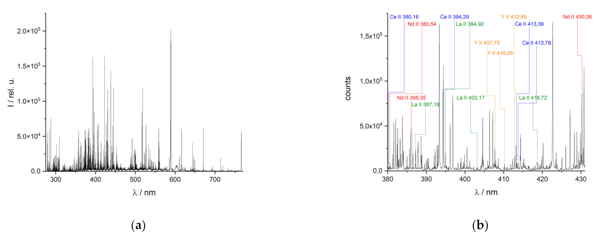
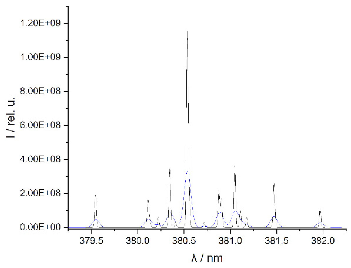
3.1. Structure of REE Spectra

LIB spectra of REE-bearing minerals are highly complex due to the line-rich REE [12,13]. The NIST LIBS database displays, e.g., 7723 lines for cerium. Furthermore, REE often occur associated with other REE. In addition, strong emission lines of other elements of the surrounding matrix contribute to the complexity of the spectra. A typical LIB spectrum of a REE-bearing mineral and an enlarged partial spectrum are displayed in Figure 2.

As a consequence of the large number, emission lines from different elements can be partially or even completely superimposed. This complicates the assignment of the lines to the numerous elements, especially in spectrometers with a lower resolution. The use of high-resolution spectrometers can reduce these problems in line evaluation (Figure 3). Compared to spectra with a resolution of ≥100 pm, spectra with a higher resolution can be obtained by spectrometers based on echelle gratings, allowing better resolved peaks to be observed. The echelle spectrometer used here has a spectral resolution of about 25–30 pm in the VIS range.

The improved resolution of the spectra enables the separation of partially superimposed lines in lower-resolution instruments and yields a more exact line position. This allows the identification of numerous lines of REE using the NIST database (Figure 2b) [39]. The identified emission lines can then be used in quantitative elemental analysis with LIBS. Two examples of unresolved features in the simulated low-resolution spectrum (resolution of 100 pm) of Nd in Figure 3 are the line triplet at 381.05 nm, which can be completely resolved in the simulated high-resolution spectrum which mimics the spectrum of an echelle spectrometer (resolution of 25 pm), and the duplet at 380.9 nm which can only be partially resolved even in the echelle spectrometer. REE lines that overlap lines of the matrix elements are unsuitable for the investigation. These lines, marked with an asterisk in

Table 1. Experimental spectral lines of analyzed REE (shown in Figure 2b) used in this work collected with the echelle spectrometer. Emission wavelengths marked with an asterisk (*) are not used in this work.

Species	Spectral Lines
Ce II	380.15 nm, 394.27 nm *, 413.38 nm, 413.76 nm
La I	418.73 nm *
La II	387.16 nm *, 394.91 nm, 403.16 nm
Nd II	380.53 nm, 386.34 nm, 430.22 nm *
Y I	410.24 nm, 407.73 nm *, 412.82 nm

below, are not included in the analyses performed in this work. The other spectral lines listed were used in the univariate and multivariate regression.

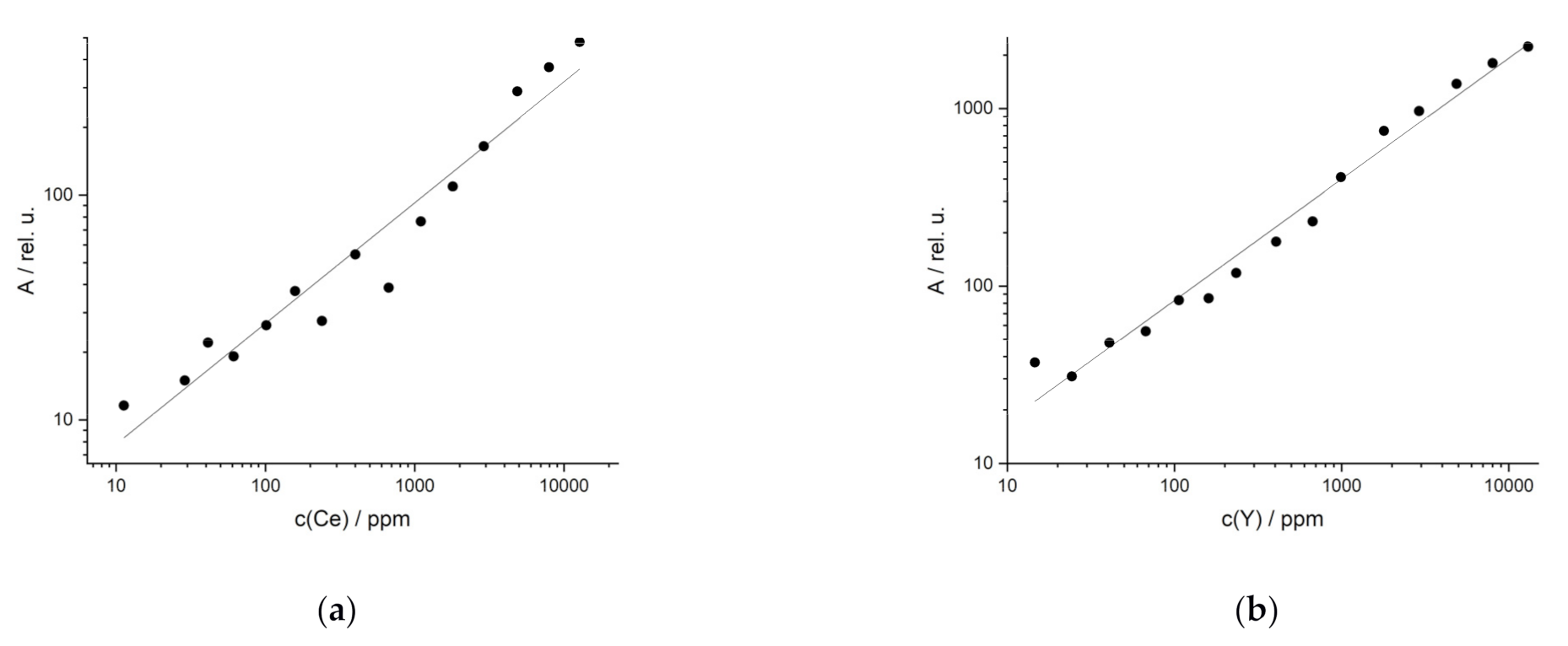
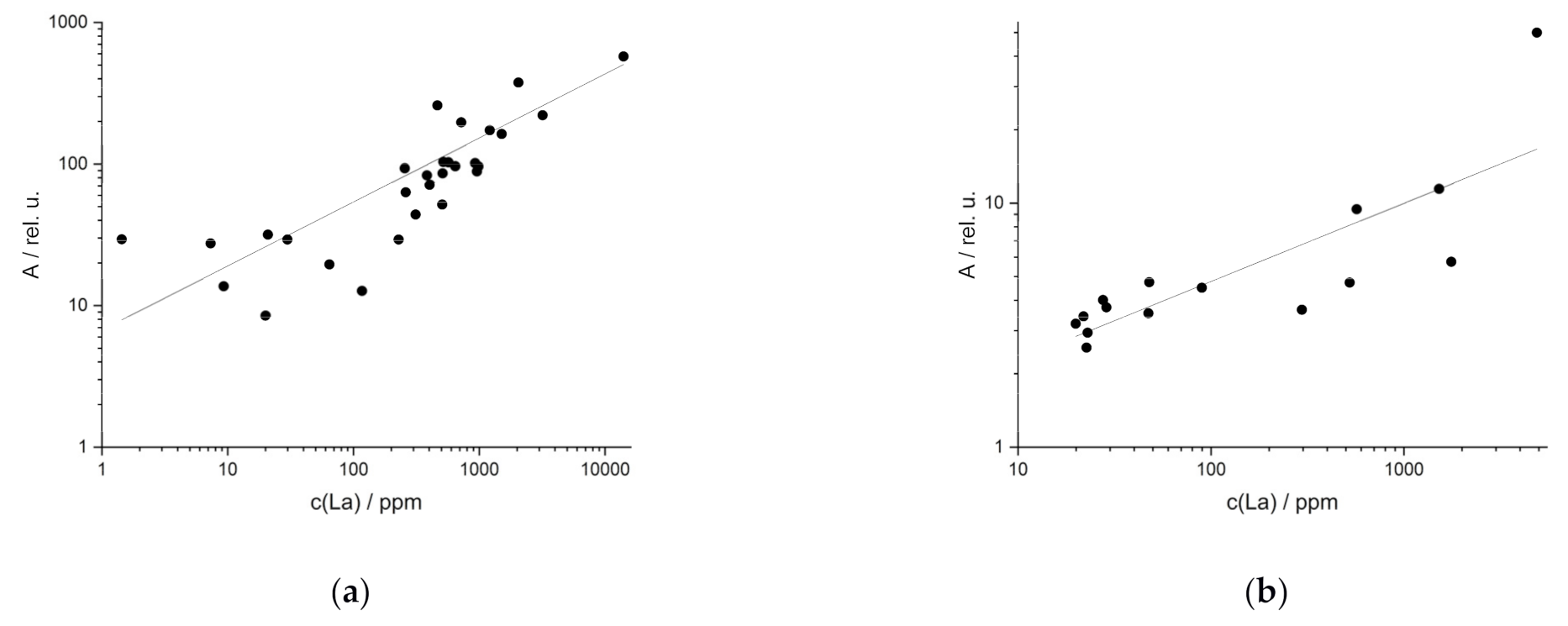
3.2. Univariate Regression

REE do not occur as native metals in nature. Rather, they occur in various rock-forming minerals [6]. This results in field samples being complex mixtures of a wide variety of elements [13]. To evaluate the influence of the matrix elements on LIB spectra of REE, univariate regression analyses were performed on the data sets of the synthetic and field samples experimentally obtained. While the matrix of the synthetic REE samples (one rock or soil) is constant, REE in field samples are embedded in various minerals, rocks or soils. The samples in this work contain Ce, La, Nd and Y at different concentrations. For each REE investigated, a regression analysis was performed at up to 3 emission lines. The corresponding coefficients of determination (R²) and limits of detection (LOD) are reported. The LOD is the quotient of three times the standard deviation of the baseline and the slope of the obtained regression line. The resulting values of LOD are shown in

Table 2. Results of univariate regression of synthetic samples of REE (Ce, La, Nd, Y) in rock and soil: wavelength, LOD and R² of best and other analyzed REE lines.

Species	λ/nm	LOD/ppm	R²	Species	λ/nm	LOD/ppm	R²
in rocks	best results			other lines
Ce II	413.76	115	0.91	Ce II	413.38	120	0.90
				Ce II	456.23	130	0.90
La II	379.08	3180	0.99	La II	399.57	7700	0.99
				La II	433.37	3500	0.99
Nd II	386.34	158	0.98	Nd II	380.53	28500	0.91
Y I	412.82	61	0.97	Y I	410.24	65	0.97
				Y II	488.36	50	0.97
in soils	best results			other lines
Ce II	413.76	285	0.99	Ce II	413.38	290	0.98
				Ce II	456.23	270	0.99
La II	404.29	160	0.97	La I	550.13	210	0.95
				La I	624.99	200	0.95
Nd II	386.34	414	0.96
Y II	488.36	227	0.98	Y II	363.31	270	0.95
				Y II	437.49	290	0.94

.

Only spectral lines which occur in the entire examined concentration range were used. Since unsuitable lines also occur for each element (Table 1), different emission lines were used for the analyses in the different matrices. In the investigated field samples, the REE content varies over several orders of magnitude (from 1 ppm up to 3%). Therefore, the presentation of the regression lines is best done by a double logarithmic plot to cover the whole concentration range. All lines investigated are summarized in Table 2 with the corresponding coefficients of determination and LOD.

3.2.1. Univariate Regression of Synthetic Samples

For synthetic REE samples of rocks, the UVR functions of the Ce line at 413.76 nm and the Nd line at 386.34 nm are shown in Figure 4 as examples. Both elements show the best regression results at these emission lines in terms of linearity, which is R² = 0.91 for Ce and R² = 0.98 for Nd. The other studied REE, La and Y, also have good coefficients of determination at the selected wavelengths: R² (La at 379.08 nm) = 0.99 and R² (Y at 412.82 nm) = 0.97.

The results of the UVR obtained for the synthetic samples in soils were similar to the synthetic minerals although the emission lines varied. Examples are the results for the REE Ce and Y in soils (Figure 5). For Ce the emission line at 413.76 nm, and for Y the line at 488.36 nm were used, respectively. Both have high coefficients of determination (R² (Ce) = 0.99, R² (Y) = 0.98). Coefficients of R² > 0.96 were also obtained for the UVR of the elements La (404.29 nm) and Nd (386.34 nm). The other reported lines of the REE in rock and soil also yield good results, but they show reduced linearity as indicated by smaller R² (R² = 0.90–0.99, Table 2). The detection limits of the REE in rock and soil are similar for most elements. Their average LOD is 200 ppm (except for La in rock, which exhibited an unusually high LOD as a result of the large spread of the data points, very likely due to matrix effects) with a standard deviation of 110 ppm. Nevertheless, the values of the LOD vary between elements and even between the matrices for one element, sometimes significantly.

3.2.2. Univariate Regression of Field REE Samples

In comparison to the synthetic samples, the UVR of the field samples of REE-bearing rocks yielded worse results. This is due to two reasons: first, the matrix, which is significantly more complex than the matrix of the synthetic samples, which consists of only one rock (serpentinite). Second, there are great matrix variations between the different sample locations. The UVR results were again evaluated on the basis of the coefficients of determination. These range from 0.43 to 0.85 for field rock samples (

Table 3. Results of univariate regression of field samples of REE (Ce, La, Nd, Y) in rocks and soils: wavelength, LOD and R² of best and other analyzed REE lines.

Species	λ/nm	LOD/ppm	R²	Species	λ/nm	LOD/ppm	R²
in rocks	best results			other lines
Ce II	413.76	218	0.79	Ce II	380.15	290	0.75
				Ce II	446.02	210	0.7
La II	408.67	199	0.82	La II	404.29	180	0.79
				La II	433.37	220	0.77
Nd II	325.91	1090	0.56	Nd II	386.34	250	0.41
				Nd II	325.91	1230	0.47
Y II	437.49	117	0.85	Y I	412.82	160	0.82
				Y II	321.68	140	0.80
in soils	best results				other lines
Ce I	594.08	359	0.51	Ce I	560.12	500	0.41
				Ce I	571.9	470	0.41
La II	404.29	294	0.52	La II	433.37	540	0.48
				La I	624.99	860	0.44
Nd II	325.91	592	0.43	Nd II	380.53	410	0.16
				Nd II	386.34	800	0.34
Y I	297.45	296	0.43	Y II	321.68	350	0.33
				Y I	410.24	600	0.20

). An example is the best La line at 408.67 nm (R² = 0.82, Figure 6a). Except for Nd, the best emission lines of the other REE investigated yield coefficients of determination around 0.80 (Table 3).

Stronger matrix effects can be observed in the UVR of field soil samples. These samples have an even higher variance in composition, which affects the LIB spectra. UVR of the best lines yields low coefficients of determination between 0.16 and 0.52 (Table 3). This is shown in Figure 6b for the regression lines of La (404.29 nm).

The average LOD for the investigated REE in field samples (soils and rocks) is 300 ppm (except for Nd in rock) with a standard deviation of 140 ppm. Thus, the LOD values are slightly higher than the LOD of the synthetic samples. Better results of the UVR analysis were obtained for those samples that have the same and a less complex matrix composition, i.e., for the synthetic samples of rock or soil. In natural field samples with strong matrix variations, multivariate methods have the potential to compensate the variations in spectral interference caused by the differences in matrix compositions and can be an alternative to the UVR.

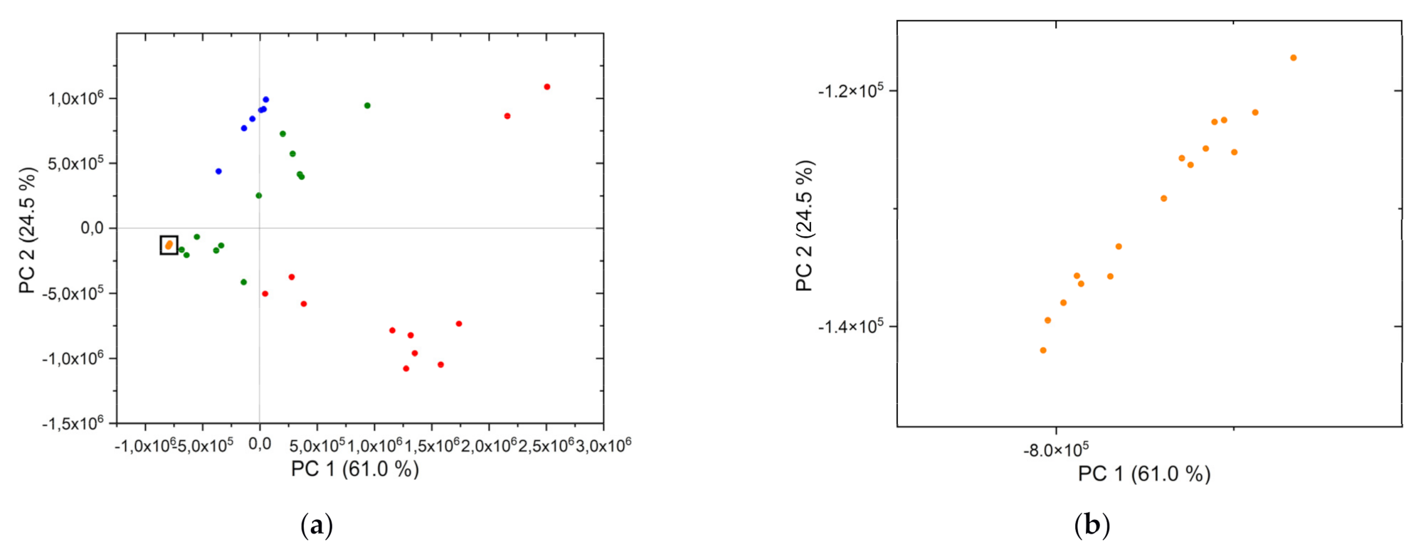
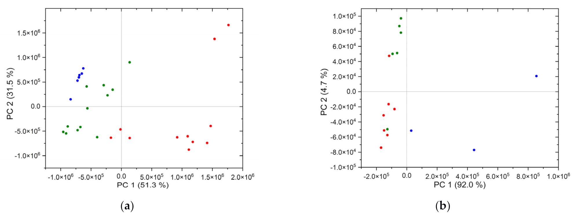
3.3. Characterization of Matrix Effects by Means of PCA

One way to investigate these influences of the matrices is to characterize the differences in the chemical composition of soil and rock. This is possible by means of unsupervised methods such as principal component analysis (PCA). For this purpose, the LIB spectra of the soils and rocks collected near the three REE deposits are investigated by PCA. The first two principal components are shown in the score plot (Figure 7). For the reference rocks, 82.8% of the variance can be explained by the first two components (Figure 7a). In the case of the reference soils, 96.7% of the variance is explained by the two components (Figure 7b). In the score plot of the rock samples (Figure 7a), the samples of the three deposits form well separated clusters, which are displayed in different colors. The samples of the individual deposit clusters also show a considerable scattering, especially in the case of the Norra Kärr samples. This allows the determination of the provenance of the samples and also indicates the strong differences in the chemical composition of the matrices within and between the deposits, which is caused by the types of rocks present in the individual deposits. All three deposits are composed of siliceous or carbonaceous rocks. However, the included minerals influence the composition and thus allow a differentiation of the deposits by PCA. The igneous rock of the Swedish Norra Kärr deposit (red) is a nepheline-bearing syenite with agpaitic composition. These samples are particularly rich in sodium and potassium. In contrast, the Olserum deposit (green) has a mainly cordierite-bearing gneiss. As a result, the siliceous rock is magnesium- and aluminum-bearing. The rocks of the Fen complex (blue) are carbonatites. Due to chemical and physical weathering processes and accompanying degradation, the data points are partly scattered over large areas even within the clusters. In addition, the widely spaced sampling locations (>50 m) contribute to the splitting of the data points. The points from the Norra Kärr deposit show the largest scatter. Here the sampling locations are up to 200 m apart. The sampled veins in Olserum are about 150 m apart.

For the soils, the interpretation of the PCA (Figure 7b) is more complex, since the soils consist not only of physically weathered rock, but also of organic matter from the biosphere and atmospheric dust [40]. Nevertheless, as in the principal component analysis of the reference rocks, a clustering of the data points according to the deposits and their separation from each other can be observed. This probably results from the rocks present. Although the sampling locations in the deposits are far apart, the data points within the PCA are not as split up as in the case of the reference rocks. This could be due to incoming organic matter and atmospheric dust during formation. Thus, the samples are possibly more homogeneous. In contrast, the strong splitting of the data points from the Fen complex (blue) is particularly striking. This is probably due to the different weathering grade of the soils.

In comparison, both PCA show similar results: data points are grouped by deposit and separated from each other. All clusters show an internal separation of the data points. The explained variance of both PCA analyses is already >82% for two principal components. Thus, it is possible to assign the present samples to a single deposit. Surprisingly, the explained variance of the reference soils is larger than that of the rocks. The reason for this could be the nature of the samples. The soil samples are in powder form and thus show a greater macroscopic homogeneity than the investigated rocks. As a result, the properties are more evenly distributed, so that the components of the PCA capture more properties. Thus, the reference soils can be explained with fewer principal components.

However, the differences in the chemical composition of the samples are also evident in both analyses. This heterogeneity of the field samples is striking in the PCA of field and synthetic samples (Figure 8a,b). In addition to the LIB spectra of the reference rocks, the spectra of the synthetic samples (Ce) were included in the analysis. From the principal component analysis (Figure 8a) it can be seen that the synthetic samples are more homogeneous. These data points (orange) are concentrated in a small area of the score plot. Nevertheless, they are not located at exclusively one point in the score plot, as the magnification in Figure 8b shows. In comparison, the data points of the field samples are distributed over a wide area in the plot. This supports our observation that the separation between the samples from different sites is caused by the differences in the chemical composition of the matrix and not by the variations in REEs concentration.

After performing PCA, it is clear that UVR is well suited for the synthetic samples because they have a more homogeneous composition. For field samples, on the other hand, univariate regression is unsuitable due to the heterogeneous matrix. For heterogeneous samples, the use of multivariate regression models is therefore examined.

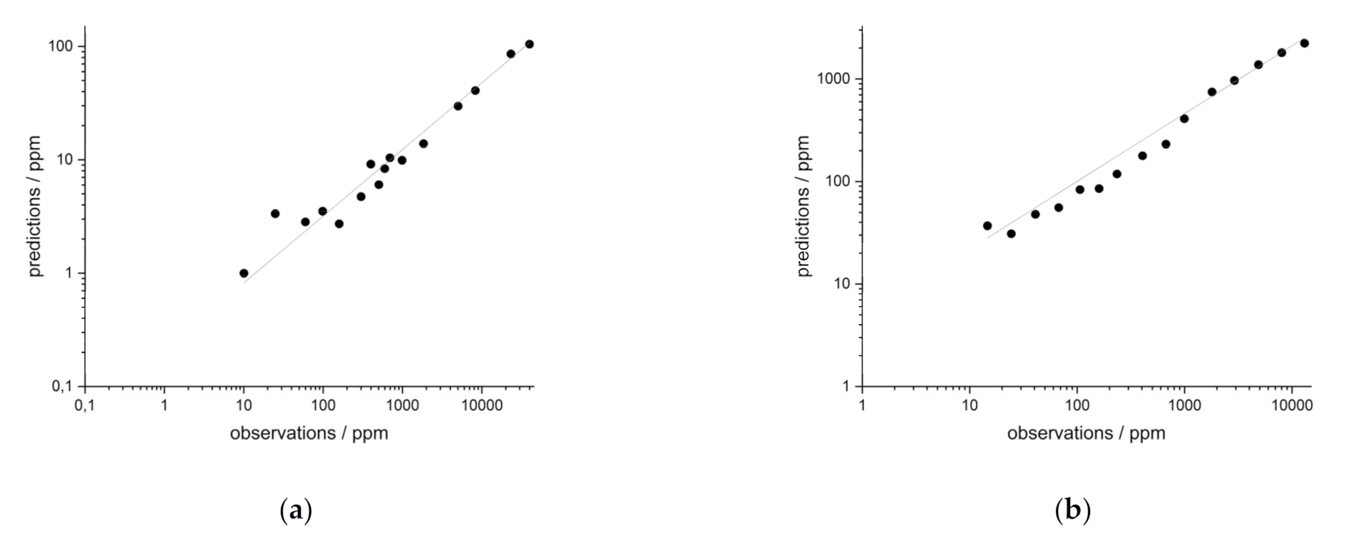
3.4. Interval Partial Least-Squares (iPLS) Regression

The multivariate method used was interval partial least-squares (iPLS) regression based on variable selection. In this method, the spectra are divided into intervals of equal spectral width. The number of intervals and the number of components were determined based on the lowest RMSE individually for each sample and are reported in

Table 4. Results of iPLS regression of synthetic samples in rocks and soils.

Species	# Intervals	Interval Width/nm	iPLS: R²	PLS: R²
	# Components	Element Line/nm	RMSECV	RMSECV
synthetical samples in rocks
Ce II	3000 intervals	0.02	0.98	0.88
VIS	10 components	507.50	1500 ppm	3719 ppm
La II	20 intervals	20.35	0.99	0.99
VIS	4 components	398.8, 399.57, 403.2, 404.29, 407.7, 408.67	490 ppm	391 ppm
Nd II	1 interval	490.56	0.98	0.96
VIS	3 components	380.53	1650 ppm	2250 ppm
Y II	3000 intervals	0.05	0.99	0.73
UV	10 components	324.20	590 ppm	5130 ppm
synthetical Samples in Soils
Ce II	2000 intervals	0.20	0.99	0.93
VIS	12 components	407.90, 408.00	280ppm	840 ppm
La II	2000 intervals	0.19	0.96	0.24
VIS	6 components	394.90	0.42%	3205 ppm
Nd II	3000 intervals	0.16	0.95	0.73
VIS	7 components	532.00	0.45%	1903 ppm
Y II / I	800 intervals	0.46	0.98	0.95
VIS	4 components	374.80, 374.90	480 ppm	827 ppm

and

Table 5. Results of iPLS regression of field samples in rocks and soils.

Species	# Intervals	Interval Width/nm	iPLS: R²
	# Components	Element Line/nm	RMSECV
field samples in rocks
Ce II	2000 intervals	0.288	0.92
VIS	18 components	639.30	1680 ppm
La I	5000 intervals	0.078	0.92
VIS	3 components	495.00	760 ppm
Nd I	400 intervals	1.30	0.89
VIS	15 components	521.30	1000 ppm
Y I	1000 intervals	0.52	0.91
VIS	4 components	552.76	870 ppm
field samples in soils
Ce II	400 intervals	1.24	0.83
VIS	12 components	502.30	1000 ppm
La II	1800 intervals	0.269	0.93
VIS	11 components	497.00	350 ppm
Nd II	1000 intervals	0.164	0.83
VIS	12 components	307.50	420 ppm
Y II	2100 intervals	0.17	0.84
VIS	11 components	371.00	200 ppm

.

The method was first tested on the more homogeneous synthetic samples. As shown by the results in Table 4, the iPLS regression provides similarly good and, in some cases, even better results than the UVR for these samples. Thus, for the synthetic samples of cerium in rock, a better coefficient of determination of 0.98, compared to the UVR (R² = 0.91, Cf. Table 2), could be obtained. An improvement of the regression could also be accomplished for yttrium (R² (iPLS) = 0.99, R² (UVR) = 0.97). For lanthanum and neodymium (Figure 9a) the coefficients of determination of iPLS regression and UVR are in the same good range.

Similar results were obtained for the synthetic soil samples (see univariate data in Table 2 and data of iPLS regression in Table 4). Figure 9b shows the iPLS results of yttrium in soils. For the investigated REE cerium, lanthanum, neodymium and yttrium, coefficients of determination between R² = 0.95–0.99 were achieved. These are similar to the R² of the UVR (R² = 0.96–0.99). The fact that the multivariate method performs as well or even better for the synthetic samples suggest that their application to heterogeneous field samples could be beneficial.

The application of iPLS regression to the heterogeneous field samples yields significantly better regression results than the UVR in all cases investigated. For samples in rock, R² > 0.91 can be obtained (Table 5). For lanthanum (Figure 10a), in contrast to the UVR (R² = 0.82), a coefficient of determination of R² = 0.92 can be achieved by iPLS regression. For neodymium, a R² of 0.98 is found by using the multivariate regression method (Figure 10b), which is also significantly better than for UVR (R² (UVR) = 0.56). Somewhat less pronounced, but equally good, are the improvements in the regressions of cerium and yttrium in rock.

The improvement of the regression is most obvious for the field samples in soils. The best coefficient of determination achieved for a UVR was R² = 0.52. All coefficients of determination obtained for iPLS regression are better than R² > 0.83 (Table 5). For lanthanum, the univariate regression value R² = 0.52 can be increased to R² = 0.93 in the multivariate regression. The improvement is similarly strong in the case of neodymium. Comparable to this are the changes in regression for yttrium and cerium.

In the iPLS regression, only the intervals containing relevant information, such as the element lines, are considered (Table 4 and Table 5). To that end, very small interval widths had to be used in most cases. The subsequent PLS regression could thus also be considered an automated UVR. Nevertheless, the iPLS regression has higher coefficients of determination than the UVR. In addition to iPLS, PLS regression of the entire spectra was also examined. However, this method was not able to provide a prediction better than guessing. This demonstrates the advantage of variable selection in iPLS. Due to the sometimes extremely narrow intervals, only parts of the relevant element lines are included in the regression. Negative effects, such as self-absorption and partial contamination of the flank of lines, are excluded, resulting in improved regressions with higher coefficients of determination [41].

In particular, the quality of the regression of the field soil samples shows the strength of the multivariate method iPLS regression chosen here. Whereas, in the univariate regression, coefficients of determination of R² = 0.47 are achieved on average, the regression can be improved to a mean R² = 0.88. In addition to selecting appropriate spectral regions that contain relevant information, variable selection also allows elimination of intervals that contain noise or other irrelevant data. This can consider the influence of matrix effects of the studied rocks and soils.

4. Summary and Conclusions

LIBS is a promising method for the detection of rare earth elements in rocks and soils, as this technique can be used to detect REE in various matrices with no or minimal sample preparation. However, the spectral influence due to the matrices is problematic. In order to consider this influence and increase the power of the analysis, multivariate methods are required, especially for heterogeneous samples. In the present work, two approaches were used to analyze the LIBS data. The first approach is the UVR based on the peak area of the relevant LIBS signals. Here, the matrix effects of the heterogeneous field samples were identified as problematic and further investigated using PCA. The influence of these effects is considered in the second approach, a multivariate method. An iPLS regression was used in which only relevant regions of the spectrum were included in the regression. This improved the predictive accuracy of the regression. The investigations show that the detection and evaluation of REE in rocks and soils is possible using LIBS in combination with multivariate iPLS regression. The use of mobile LIB spectrometers can thus potentially enable the exploration of new REE deposits.

To increase the predictive power of the method, further investigations should be extended by samples from other deposits. Of particular interest here are REE-bearing samples, which have different accompanying matrices. For future studies, larger intervals and combinations of individual intervals could be used with a smaller number of components. For possible applications in the field, the use of a mobile spectrometer should be further investigated. Should these investigations prove successful, the transfer of the methods developed here into the field could be a promising possibility.

References

1. Altenberger, U.; Oberhänsli, R. Vom Atom Zum Hightec-Produkt. Minerale Der Seltenerdelemente Als Rohstoffe. PdN Chem. Schule/Mineralien Erze 2012, 7, 6–12. [Google Scholar]
2. Sicius, H. Seltenerdmetalle: Lanthanoide Und Dritte Nebengruppe; Essentials; Springer Fachmedien Wiesbaden: Wiesbaden, Germany, 2015; ISBN 978-3-658-09839-1. [Google Scholar]
3. Balaram, V. Rare Earth Elements: A Review of Applications, Occurrence, Exploration, Analysis, Recycling, and Environmental Impact. Geosci. Front. 2019, 10, 1285–1303. [Google Scholar] [CrossRef]
4. Marscheider-Weidemann, F.; Langkau, S.; Hummen, T.; Erdmann, L.; Tercero Espinoza, L.; Angerer, G.; Marwede, M.; Benecke, S. Rohstoffe für Zukunftstechnologien 2016.—DERA Rohstoffinformationen 28: 353 S., Berlin. Available online: https://www.deutsche-rohstoffagentur.de/DERA/DE/Downloads/Studie_Zukunftstechnologien-2016.pdf?__blob=publicationFile&v=3 (accessed on 6 November 2021).
5. Gaft, M.; Raichlin, Y.; Pelascini, F.; Panzer, G.; Motto Ros, V. Imaging Rare-Earth Elements in Minerals by Laser-Induced Plasma Spectroscopy: Molecular Emission and Plasma-Induced Luminescence. Spectrochim. Acta Part B At. Spectrosc. 2019, 151, 12–19. [Google Scholar] [CrossRef]
6. Walters, A.; Lusty, P.; Hill, A. Rare Earth Elements; British Geological Survey: Nottingham, UK, 2011. [Google Scholar]
7. Mehmood, M. Rare Earth Elements—A Review. J. Ecol. Nat. Resour. 2018, 2. [Google Scholar] [CrossRef]
8. Romppanen, S.; Häkkänen, H.; Kaski, S. Singular Value Decomposition Approach to the Yttrium Occurrence in Mineral Maps of Rare Earth Element Ores Using Laser-Induced Breakdown Spectroscopy. Spectrochim. Acta B 2017, 134, 69–74. [Google Scholar] [CrossRef]
9. Erdmann, L.; Behrendt, S. Kritische Rohstoffe Für Deutschland. Izt 2011, 1–13. Available online: https://www.izt.de/fileadmin/publikationen/54416.pdf (accessed on 6 November 2021).
10. Brown, T.J. World Mineral Production; British Geological Survey: Nottingham, UK, 2020; ISBN 9780511763175. [Google Scholar]
11. Goodenough, K.M.; Wall, F.; Merriman, D. The Rare Earth Elements: Demand, Global Resources, and Challenges for Resourcing Future Generations. Nat. Resour. Res. 2018, 27, 201–216. [Google Scholar] [CrossRef] [Green Version]
12. Müller, S.; Meima, J.A.; Rammlmair, D. Detecting REE-Rich Areas in Heterogeneous Drill Cores from Storkwitz Using LIBS and a Combination of K-Means Clustering and Spatial Raster Analysis. J. Geochem. Explor. 2021, 221, 106697. [Google Scholar] [CrossRef]
13. Bhatt, C.R.; Jain, J.C.; Goueguel, C.L.; McIntyre, D.L.; Singh, J.P. Determination of Rare Earth Elements in Geological Samples Using Laser-Induced Breakdown Spectroscopy (LIBS). Appl. Spectrosc. 2018, 72, 114–121. [Google Scholar] [CrossRef]
14. Zawisza, B.; Pytlakowska, K.; Feist, B.; Polowniak, M.; Kita, A.; Sitko, R. Determination of Rare Earth Elements by Spectroscopic Techniques: A Review. J. Anal. At. Spectrom. 2011, 26, 2373–2390. [Google Scholar] [CrossRef]
15. Fabre, C.; Devismes, D.; Moncayo, S.; Pelascini, F.; Trichard, F.; Lecomte, A.; Bousquet, B.; Cauzid, J.; Motto-Ros, V. Elemental Imaging by Laser-Induced Breakdown Spectroscopy for the Geological Characterization of Minerals. J. Anal. At. Spectrom. 2018, 33, 1345–1353. [Google Scholar] [CrossRef]
16. Labutin, T.A.; Zaytsev, S.M.; Popov, A.M.; Zorov, N.B. A Novel Approach to Sensitivity Evaluation of Laser-Induced Breakdown Spectroscopy for Rare Earth Elements Determination. J. Anal. At. Spectrom. 2016, 31, 2223–2226. [Google Scholar] [CrossRef]
17. Anderson, R.B.; Morris, R.V.; Clegg, S.M.; Humphries, S.D.; Wiens, R.C.; Bell III, J.F.; Mertzman, S.A. Partial Least Squares and Neural Networks for Quantitative Calibration of Laser-Induced Breakdown Spectroscopy (LIBs) of Geologic Samples. In Proceedings of the Lunar and Planetary Science, The Woodlands, TX, USA, 1–5 March 2010. [Google Scholar]
18. Erler, A.; Riebe, D.; Beitz, T.; Löhmannsröben, H.G.; Gebbers, R. Soil Nutrient Detection for Precision Agriculture USING Handheld Laser-Induced Breakdown Spectroscopy (LIBS) and Multivariate Regression Methods (PLSR, Lasso and GPR). Sensors 2020, 20, 418. [Google Scholar] [CrossRef] [Green Version]
19. Andersen, C.M.; Bro, R. Variable Selection in Regression—A Tutorial. J. Chemom. 2010, 24, 728–737. [Google Scholar] [CrossRef]
20. Nørgaard, L.; Saudland, A.; Wagner, J.; Nielsen, J.P.; Munck, L.; Engelsen, S.B. Interval Partial Least-Squares Regression (iPLS): A Comparative Chemometric Study with an Example from near-Infrared Spectroscopy. Appl. Spectrosc. 2000, 54, 413–419. [Google Scholar] [CrossRef]
21. Sánchez-Esteva, S.; Knadel, M.; Kucheryavskiy, S.; de Jonge, L.W.; Rubæk, G.H.; Hermansen, C.; Heckrath, G. Combining Laser-Induced Breakdown Spectroscopy (LIBS) and Visible near-Infrared Spectroscopy (Vis-NIRS) for Soil Phosphorus Determination. Sensors 2020, 20, 5419. [Google Scholar] [CrossRef]
22. Andersson, S.S.; Wagner, T.; Jonsson, E.; Fusswinkel, T.; Leijd, M.; Berg, J.T. Origin of the High-Temperature Olserum-Djupedal REE-Phosphate Mineralisation, SE Sweden: A Unique Contact Metamorphic-Hydrothermal System. Ore Geol. Rev. 2018, 101, 740–764. [Google Scholar] [CrossRef]
23. Fullerton, W. REE Mineralisation and Metasomatic Alteration in the Olserum Metasediments. Master’s Thesis, Lund University, Lund, Sweden, 2014. [Google Scholar]
24. Russell, R.V. Porphyroblastic Differentiation in Fleck Gneiss from Västervik, Sweden. Geologiska Föreningen i Stockholm Förhandlingar 1969, 91, 217–282. [Google Scholar] [CrossRef]
25. Gavelin, S. The Västervik Area in South-Eastern Sweden. Studies in Proterozoic Sedimentation, High-Grade Metamorphism and Granitization; Sveriges Geologiska Undersökning: Uppsala, Sweden, 1984; Volume 32. [Google Scholar]
26. Adamson, O.J. The Petrology of the Norra Kärr District: An Occurrence of Alkaline Rocks in Southern Sweden. GFF 1944, 437, 113–255. [Google Scholar] [CrossRef]
27. Sieg, L. Distribution of Rare Earth Elements in Rocks, Soils and Plants from Olserum and Norra Kärr, Sweden. Master’s Thesis, University of Potsdam, Potsdam, Germany, 2016, unpublished. [Google Scholar]
28. Sjöqvist, A.S.L.; Cornell, D.H.; Andersen, T.; Christensson, U.I.; Berg, J.T. Magmatic Age of Rare-Earth Element and Zirconium Mineralisation at the Norra Kärr Alkaline Complex, Southern SWEDEN, Determined by U–Pb and Lu–Hf Isotope Analyses of Metasomatic Zircon and Eudialyte. Lithos 2017, 294–295, 73–86. [Google Scholar] [CrossRef]
29. Gorbatschev, R. The Transscandinavian Igneous Belt—Introduction and Background; Högdahl, K., Eklund, U.B., Andersson, O., Eds.; Geological Survey of Finland: Espoo, Finland, 2004; ISBN 9516908896. [Google Scholar]
30. Atanasova, P.; Marks, M.A.W.; Heinig, T.; Krause, J.; Gutzmer, J.; Markl, G. Distinguishing Magmatic and Metamorphic Processes in Peralkaline Rocks of the Norra Kärr Complex (Southern Sweden) Using Textural and Compositional Variations of Clinopyroxene and Eudialyte-Group Minerals. J. Petrol. 2017, 58, 361–384. [Google Scholar] [CrossRef] [Green Version]
31. Sjöqvist, A.S.L. Agpaitic Rocks of the Norra Kärr Alkaline Complex: Chemistry, Origin, and Age of Eudialyte-Hosted Zirconium and Rare-Earth Element Ore. Licentiate Thesis, University of Gothenburg, Gothenburg, Sweden, 2015. [Google Scholar]
32. Törneboh, A.E. Katapleiitsyenit, En Nyupptäckt Varietet Af Nefelinsyenit I Sverige. Geologiska Föreningen i Stockholm Förhandlingar 1906, 28, 415–417. [Google Scholar] [CrossRef]
33. Andersen, T. Magmatic Fluids in the Fen Carbonatite Complex, S.E. Norway. Contrib. Mineral. Petrol. 1986, 93, 491–503. [Google Scholar] [CrossRef]
34. Andersen, T. Compositional Variation of Some Rare Earth Minerals from the Fen Complex (Telemark, SE Norway): Implications for the Mobility of Rare Earths in a Carbonatite System. Mineral. Mag. 1986, 50, 503–509. [Google Scholar] [CrossRef] [Green Version]
35. Tilley, C.E. Die Eruptivgesteine Des Kristianiagebietes. IV: Das Fengebiet in Telemark, Norwegen. By, W.C. Brøgger. Vid. Selsk. Skrifter, I.M.N.Kl. No. 9, pp. 1–408. 1920. Geol. Mag. 1921, 58, 549–554. [Google Scholar] [CrossRef] [Green Version]
36. Ließmann, W. Der Karbonatit-Alkaligesteins-Komplex von Fen. Aufschluss 2004, 55, 305–320. [Google Scholar]
37. Mitchell, R.H.; Brunfelt, A.O. Rare Earth Element Geochemistry of the Fen Alkaline Complex, Norway. Contrib. Mineral. Petrol. 1975, 52, 247–259. [Google Scholar] [CrossRef]
38. Köllner, N. Verwitterungsprofile Des FEN-Komplexes, Südnorwegen. Diploma Thesis, University of Potsdam, Potsdam, Germany, unpublished. 2015. [Google Scholar]
39. Kramida, A.; Ralchenko, Y.; Reader, J.; NIST ASD Team. NIST Atomic Spectra Database (Version 5.8) 2020; National Institute of Standards and Technology: Gaithersburg, MD, USA, October 2020. [Google Scholar]
40. Grotzinger, J.; Jordan, T. Press/Siever Allgemeine Geologie; Springer Spektrum: Heidelberg, Germany, 2017; ISBN 9783662483411. [Google Scholar]
41. Guezenoc, J.; Bassel, L.; Gallet-Budynek, A.; Bousquet, B. Variables Selection: A Critical Issue for Quantitative Laser-Induced Breakdown Spectroscopy. Spectrochim. Acta Part B At. Spectrosc. 2017, 134, 6–10. [Google Scholar] [CrossRef]
Figure 1. Maps of (a) all investigated deposits and (b) sample localities in Norra Kärr, Sweden.
Minerals 11 01379 g001
Figure 2. Representative LIB spectrum of a monazite-xenotime-apatite-bearing vein: (a) the entire spectrum (λ = 275–750 nm) and (b) a partial spectrum (λ = 380–430 nm) with important REE emission lines.
Minerals 11 01379 g002
Figure 3. Spectra of Nd (element peak at 380.5 nm) simulated on the basis of the NIST database [39] with a spectral resolution of 100 pm (blue line) and 25 pm (black line).
Minerals 11 01379 g003
Figure 4. Univariate regression of synthetic samples in rock from (a) Ce (R2 (413.76 nm) = 0.91) and (b) Nd (R2 (386.34 nm) = 0.98).
Minerals 11 01379 g004
Figure 5. Univariate regression of synthetical samples in soil of (a) Ce (R2 (413.76 nm) = 0.99) and (b) Y (R2 (488.36 nm) = 0.98).
Minerals 11 01379 g005
Figure 6. Univariate regression of field samples (a) in rocks from La (R² (408.67 nm) = 0.82) and (b) in soils from La (R² (404.29 nm) = 0.52).
Minerals 11 01379 g006
Figure 7. (a) PCA of reference rocks (VIS, raw), (b) PCA of reference soils (VIS, raw): blue—Fen complex, green—Olserum, red—Norra Kärr.
Minerals 11 01379 g007
Figure 8. (a) PCA of reference rock and synthetic samples (Ce), (b) magnification of area with synthetic samples (Ce): blue Fen complex, green Olserum, red Norra Kärr, orange synthetic samples (Ce).
Minerals 11 01379 g008
Figure 9. iPLS regression of synthetic samples(a) in rock of Nd and (b) in soils of Y.
Minerals 11 01379 g009
Figure 10. iPLS regression of field samples in rocks of (a) La and (b) Nd.
Minerals 11 01379 g010