Fumarolic Pathways Were Structurally Controlled by a Strike-Slip Fault System Beneath the Bishop Tuff, Bishop, California

Abstract

The Volcanic Tableland, a plateau at the northern end of Owens Valley, CA, is capped by the rhyolitic Bishop Tuff. It hosts many tectonic and volcanic landforms, including hundreds of fault scarps, large joint sets, and inactive fumarolic mounds and ridges. The 1986 Chalfant Valley earthquake sequence shed light on a blind strike-slip fault system beneath the Bishop Tuff. The spatial relationships of the volcanic and tectonic structures have previously been well documented, however, the mechanisms of formation of structures and their enhancement as fumarolic pathways remain largely unexplored. We collected fault kinematic indicators, joint orientations, and documented fumarolic alterations of microcrystalline quartz in the Bishop Tuff and combined those field observations with fault response modeling to assess whether strike-slip activity played a key role in the development of fumarolic pathways. We found field evidence of dip-slip and strike-slip faulting that are consistent with the overall transtensional regional tectonics. Our modeling indicates that a blind strike-slip fault system would dilate joints in the overlying Bishop Tuff with preferred orientations that match observed orientations of joints along which fumarolic activity occurred. Our results imply that the localization of fumaroles was tectonically controlled and that fault activity in the valley floor likely initiated prior to tuff emplacement.

1. Introduction

The type and involved mechanisms of fracturing in volcaniclastic sequences, such as the Bishop Tuff, depend on rock properties governed by the degree of welding of the rock [1], with densely-welded tuff accommodating brittle deformation via discrete fracturing, and poorly or non-welded tuffs frequently displaying tabular, porosity-reducing deformation bands (e.g., [2,3,4]). Both types of fractures are known to affect subsurface fluid flow, as they either form pathways for or perturb fluids. Therefore, characterizations of fracture networks in volcaniclastic rock and how fluids circulate through them is key for understanding fracture and fault sealing in general. The study of fracture flow and fracture sealing both are of economic interest, as resources, such as groundwater, ores, or petroleum migrate or accumulate along fractures. Here, we document and analyze a fracture network consisting of several sets of joints and faults in the Bishop Tuff and study its relation to hydrothermal fluid migration associated with most recent supervolcanic eruption of the Long Valley Caldera, CA, USA. Characterizations of fracture flow in such neotectonic and active volcanic settings contribute toward forecasting potential hazards and allow tying ancient tectonic and volcanic activity to observed physical or compositional aspects of mineralized fractures.

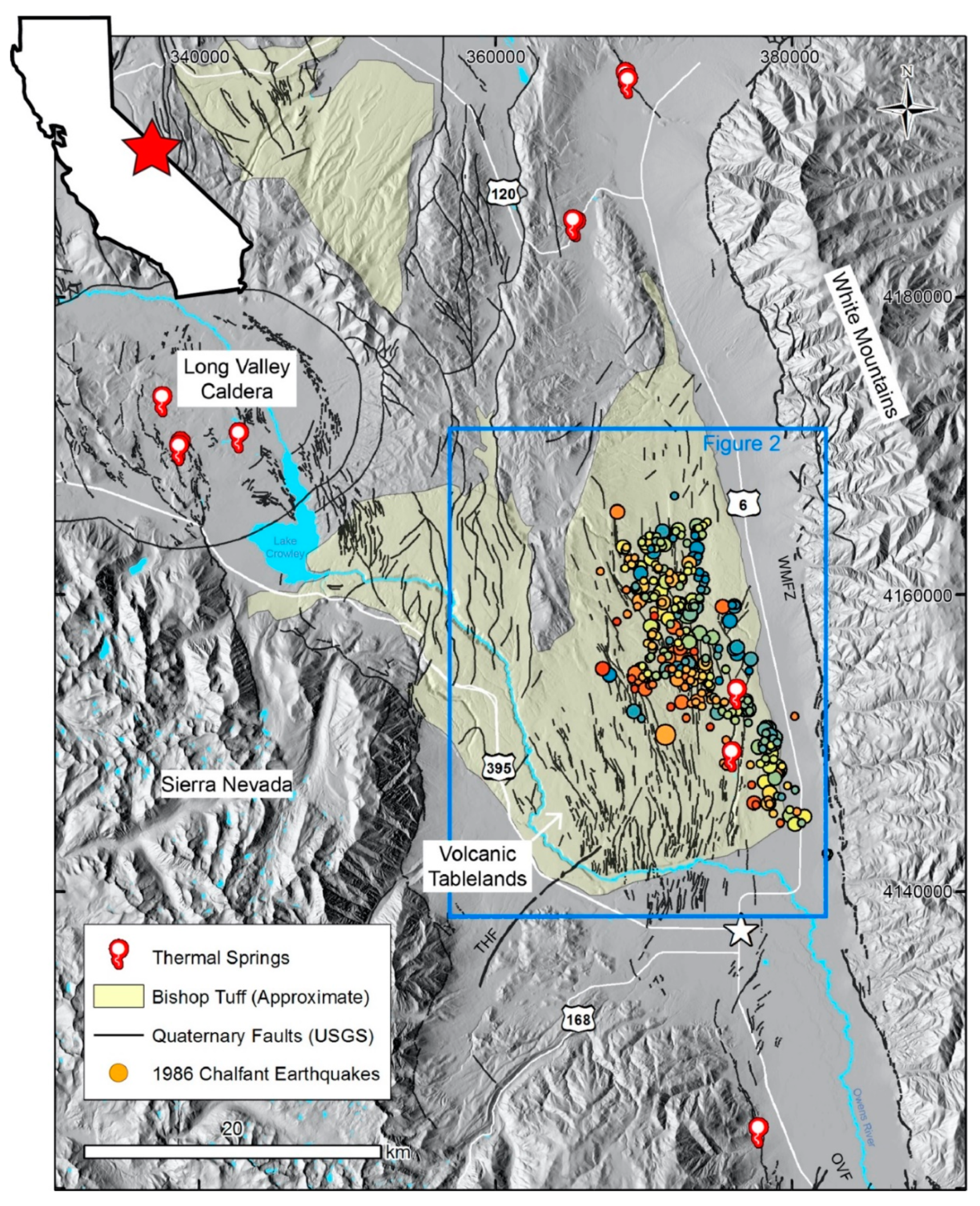
1.1. Tectonic Setting

Northern Owens Valley, where our field site is located, lies at the junction between the western margin of the Basin and Range province, the Long Valley Caldera, and the Sierra Nevada microplate (Figure 1). Owens Valley is an elongate valley that trends roughly northwest-southeast, lying between the Sierra Nevada and the White-Inyo mountains, along the western edge of the Basin and Range province (e.g., [5]). Major faults that parallel the trend of Owens valley, such as the White Mountain Fault Zone and the Owens Valley Fault, accommodate substantial extension and dextral slip (e.g., [5]) as part of the Walker Lane Belt that accounts for ~20–25% of the relative motion between the Pacific and North American plates (e.g., [6]). Northern Owens Valley has a half-graben geometry [5,7] flanked on the east by the west-dipping White Mountain Fault Zone (Figure 1) that displays up to 8 km of dip-slip displacement [5]. The fault zone has a complex history, accommodating east-west extension starting in the middle Miocene followed by dextral transtension associated with Walker Lane Belt in the Pliocene [5].

The Volcanic Tableland is a topographic plateau at the northern end of the Owens Valley, just north of Bishop, California (Figure 1). It is capped by the 758.9 + 1.8 ka rhyolitic Bishop Tuff [8,9], a layered ignimbrite atop a basal plinian fall deposit that formed from a series of nuées ardentes following the collapse of the Long Valley Caldera [10,11,12,13,14].

The tuff itself has been subdivided into two packages, representing two subsequent stages of the Long Valley Caldera eruptive sequence [13,15] and we follow the same naming conventions for units of the Bishop Tuff that were established in these references. The two packages exhibit a proximal (Ig1) and distal (Ig2) relationship from the caldera center. Ig2 shows a thickness of ~70−150 m on its southern margin, forms the Volcanic Tableland, and it is the rock unit in which the fractures reported in this study occur. It is further divided into a moderately to densely welded cap (Ig2Eb), and an underlying non- to poorly-welded tuff (Ig2Ea) [13]. Three zones of vapor-phase crystallization (Ig2Ec) overlie densely welded and devitrified units in the tuff, capping parts of the Volcanic Tableland [13,16]. These zones were formed from volatiles released during devitrification, as SiO₂ and anhydrous feldspars formed from the hot ash and pumice present in lower units of the ignimbrite [17].

Expulsion of volatiles during devitrification of tuff [17], meteoric water introduced into cooling tuff [18], or water and ice at the base of the emplaced tuff [10] are factors that could have led to fumarolic activity on the Volcanic Tableland. Hydrothermal and vapor-phase alteration associated with fumarolic activity indurated the loose, non-welded tuff at the top of the ignimbrite sequence to form a zone of vapor-phase alteration [13,16]. Non-welded ash that was not affected by fumarolic activity, was later stripped to the top of the indurated vapor-phase zone by erosive processes [10,16]. Today, domical mounds and elongated ridges on the surface of the tableland represent fossil fumarolic features that once behaved as loci of intense vapor-phase and hydrothermal activity [18].

Since its emplacement, the Bishop Tuff has been structurally modified by the formation of deep-rooted vertical conjugate joints (as seen exposed along Owens River Gorge), shallow-rooted curvilinear cooling joints, and columnar joints in areas of enhanced cooling and vapor-phase alteration [16]. Joints in the Bishop Tuff have both thermal and tectonic origins, among which a series of northeast and northwest striking conjugate joints are the most prominent of all joints in the area. Bateman [10] suggested that these were conjugate shear planes formed from a regional horizontal principal stress, similar to the conjugate joints observed in the Mesozoic granitoids of the Sierra Nevada and Tungsten Hills. Likewise, Sheridan [16] observed offsets and minor slickensides along the surfaces of conjugate joints, indicating that they are shear fractures that formed after welding increased the competency of the tuff sheet. Fumarolic activity has utilized conjugate joints, and evidence indicates that the joints extend vertically into the tuff sequence, localizing vapor-phase alteration along the joint walls [16]. As a result of the increased heat flow from rising fumarolic vapors, columnar joints radiate outwards from vertical conjugate joints in upper units of the tuff [16,18]. On a smaller (outcrop) scale, curvilinear cooling joints have formed after vapor-phase alteration was complete because they show no signs of alteration [16]. Cooling joints have variable orientations (with curving dips and strikes) that make polygonal patterns, and they often approach orthogonal intersections with larger conjugate joints, which indicates that they likely formed from the release of thermal stress as the tuff continued to cool [16].

Figure 1. Geographic overview of northern Owens Valley, with its location in California shown in upper left corner, shown as a hillshade map with westward illumination in Universal Transverse Mercator projection (UTM zone 11N). The map highlights the extent of the Bishop Tuff (approximated after Luedke and Smith [19]), quaternary faults plotted from the USGS fault database, and active thermal springs. Please note locations of the White Mountain Fault Zone (WMFZ), Owens Valley Fault (OVF), and Tungsten Hills Fault (THF) as major structures of the area. The epicenters from the 1986 Chalfant Earthquake Sequence are shown as colored circles, with circle sizes representing earthquake magnitude and colors representing depth. Smallest circles represent Magnitudes 3 whereas the largest circles show the events exceeding Magnitudes 6. Blue circles show the shallowest quakes at depths around ~0.8 to 3.8 km whereas red circles indicate the deepest quakes at 8.6 to 15 km. The town of Bishop is indicated by the white star.

Figure 1. Geographic overview of northern Owens Valley, with its location in California shown in upper left corner, shown as a hillshade map with westward illumination in Universal Transverse Mercator projection (UTM zone 11N). The map highlights the extent of the Bishop Tuff (approximated after Luedke and Smith [19]), quaternary faults plotted from the USGS fault database, and active thermal springs. Please note locations of the White Mountain Fault Zone (WMFZ), Owens Valley Fault (OVF), and Tungsten Hills Fault (THF) as major structures of the area. The epicenters from the 1986 Chalfant Earthquake Sequence are shown as colored circles, with circle sizes representing earthquake magnitude and colors representing depth. Smallest circles represent Magnitudes 3 whereas the largest circles show the events exceeding Magnitudes 6. Blue circles show the shallowest quakes at depths around ~0.8 to 3.8 km whereas red circles indicate the deepest quakes at 8.6 to 15 km. The town of Bishop is indicated by the white star.

Faulting on the Volcanic Tableland is extensive (Figure 1), and has been the subject of many previous research efforts because it not only preserves a record of the structural evolution of the northern Owens Valley since the emplacement of the Bishop Tuff (e.g., [10,20,21,22]) but also allows for characterizations of fault geometry and growth [23,24,25,26,27]. In general, faults strike between 340° and 350°, showing dips of ~60° (east and west) that were estimated from topographic profiles across the faults due to the absence of accessible or exposed fault surfaces, and many faults occur in left-stepping en echelon arrangements with relay ramps evident where fault tips overlap [20].

The kinematics of the faults on the Volcanic Tableland are found to be primarily dip-slip resulting from east-west valley extension and the subsequent down warping of the Bishop Tuff along the White Mountain Fault Zone [20,21,23,27]. North trending fault strikes roughly perpendicular with regional extension and the lack of accessible, well-preserved fault surfaces and kinematic indicators have contributed toward this conclusion. Other research has suggested that the northwestern en echelon arrangement of normal faults on the Volcanic Tableland accommodates regional transtensional dextral shear [10,28,29,30,31,32].

In late July 1986, a Magnitude 6.3 earthquake and its many associated fore- and aftershocks occurred in the Chalfant Valley area north of Bishop. It became known and is now widely referred to as the 1986 Chalfant Valley earthquake sequence [29] (Figure 1). The earthquake sequence revealed the presence of a conjugate blind strike-slip system buried beneath the tableland, which provided further evidence of transtensional dextral shear being manifested across the Volcanic Tableland. Following the earthquake, Lienkaemper et al. [33] recorded en echelon patterns preserved in loose sediments atop the tableland that were similar to the distribution of normal faults in the area, but their findings lacked concrete evidence directly linking kinematics in the tuff to the underlying strike-slip fault system. A tectonic link between the tuff and underlying valley floor has also been inferred in several other studies. To explain differences in fault displacement distributions, Dawers et al. [23] postulated that the mechanical contrast between poorly consolidated valley fill material and the overlying tuff allows for normal faulting at the surface that is kinematically distinct from strike-slip faulting in the basement. Distributed deformation was suggested by Lienkaemper et al. [33] to occur in the alluvium beneath the Bishop Tuff, differentiating between simple shear at seismogenic depth and fault-guided slip on the existing structures of the Volcanic Tableland, ultimately linking tableland deformation to many deep seismic events similar to the Chalfant Valley earthquake sequence. Furthermore, Pinter [20] discovered a ~2 m undegraded fault surface that preserved a pre-rupture soil profile, which was argued to be indicative of the tableland faults being coseismic with earthquake ruptures capable of producing surface displacement of the same magnitude.

The combination of faults and conjugate joints forms a complex, pervasive structural network. As a result, groundwater migration and storage in the region is largely controlled by these structures as they behave both as lateral conduits for subsurface flow into aquifers, and vertical conduits for capturing surface flow and emitting active thermal springs [34] (Figure 1). Hydrologic data indicate that the regional tectonic setting which governed the 1986 Chalfant Valley earthquake sequence had a dominant effect on the present-day hydrothermal activity in the Volcanic Tableland and nearby Long Valley Caldera [34,35].

1.2. Hypothesis

Observations of (1) focal mechanisms from the 1986 Chalfant Valley earthquake sequence revealed a blind conjugate strike-slip fault system that is interpreted to have influenced structures in the tuff [28,29,30,31,36], (2) fault scarps within the tuff curving to a dominant northwestern trend across the field site (Figure 2) coinciding with the mapped distribution of earthquake epicenters (Figure 1), and (3) the collocation of present-day hydrothermal and tectonic activities [34,35] together indicate that tectonic and hydrothermal activities are closely linked. The combination of these observations indicates that the strike-slip system is very likely to have structurally affected the Bishop Tuff and how fluids migrated through it. However, previous work has not specifically addressed the role of the blind strike-slip system relative to the post-emplacement evolution of the Bishop Tuff. We therefore hypothesize that the blind strike-slip system was active prior to the 1986 Chalfant Valley earthquake sequence, that it is expressed at the surface, and that associated tectonic activity played a key role in the structural development and enhancement of pathways for fumarolic activity that formed the many mounds and ridges on the Volcanic Tableland. To test this hypothesis, we carried out field work to record and characterize the nature and locations of mineralization and fumarolic activity and relate them to the fracture network and tectonic setting of the region via fault response modeling.

2. Materials and Methods

We carried out field work that was informed by prior reconnaissance of and mapping on publicly available remote sensing data, including 1 m/px National Agriculture Imagery Program (NAIP) digital georectified images and digital elevation models with 1 and 10 m/px resolutions from the National Center for Airborne Laser Mapping and USGS, respectively. In the field, we recorded structural orientations of joints and fault surfaces, using the Midland Valley’s FieldMove Clino application (version 2.3.3). Fault surfaces were identified by the presence of slip indicators (e.g., slickenlines and grooves), the orientation of which were also recorded. Coordinates of each observation were recorded in the application, as were any applicable field notes. All fault and joint orientation data are available in the supplementary materials of this manuscript (Tables S1 and S2). To assess the relationship between faults, joints, and fumarole development, observations were recorded where faults cut fumaroles, or where joints showed noticeable fumarolic alterations and minerlizations. Outcrops and hand samples of the Bishop Tuff were carefully described in the field. Scaled photographs were taken of all relevant observations including fault surfaces, slickenlines, joints, fumarolic features, tuff morphology, and outcrops. Important field photographs are numbered (as supplementary images 1 to 12 in Figure S1), geo-tagged, and available with captions as *.KMZ file in the supplementary materials of this paper (Figure S1). Hand samples of hydrothermally-altered tuff were collected from 37 locations and 9 thin sections were prepared for petrographic characterization of the fumarolic alteration. The localities of all field observations are also presented in Figure 2. Field data were then processed for fault kinematic analysis with the FaultKin software [37] and stress analysis using Midland Valley’s Move2018 software suite (now managed by Petroleum Experts).

3. Results

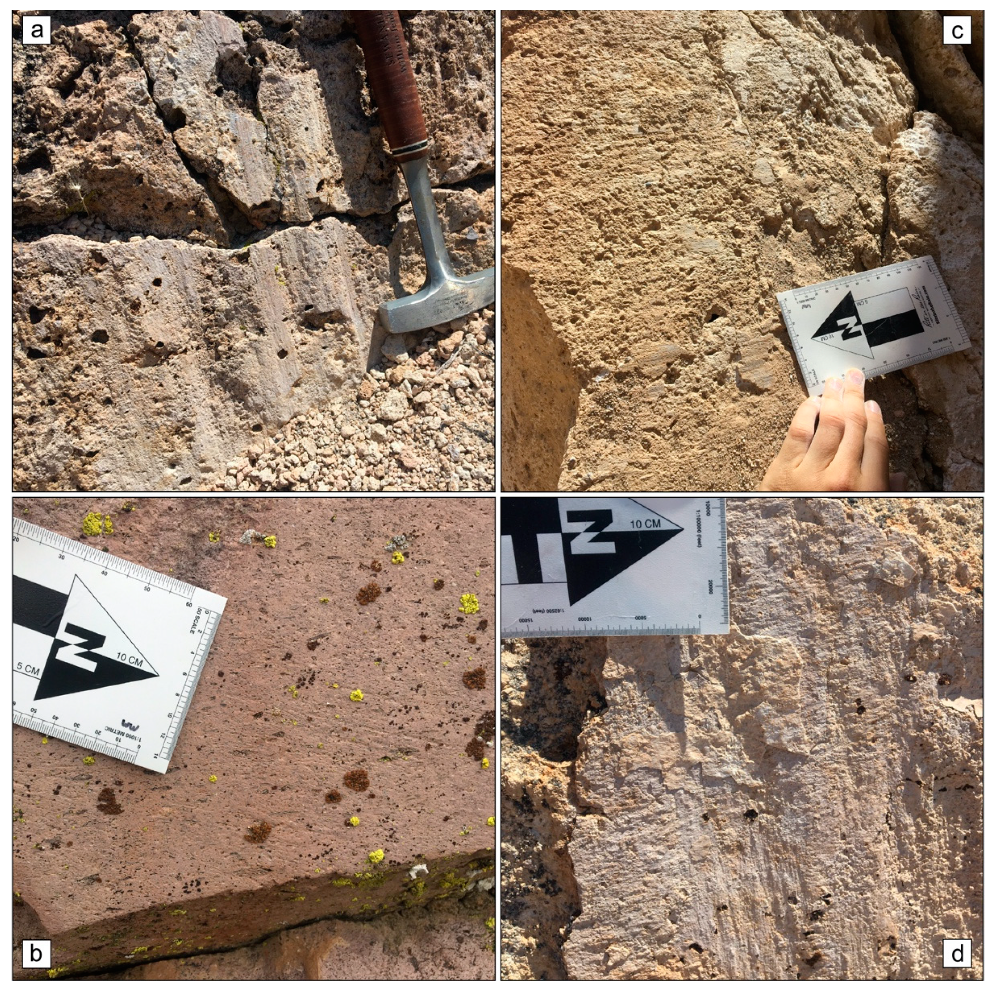
3.1. A Characterization of the Fracture Network in the Bishop Tuff

3.1.1. Joints

We identified conjugate joints as well as columnar and irregular cooling joints on the Volcanic Tableland during fieldwork (Figure 3). The largest joints occurring on the Volcanic Tableland are vertically dipping conjugate joints that strike NE and NW. Across the southern half of the field site, where they are best exposed, their lengths can be mapped to extend for hundreds of meters and they can be observed to extend vertically up to ~100 m in the Owens River Gorge (Figure 3a). Fumarolic mounds on the tableland frequently align into long linear chains (image 2 in Figure S1) that follow the strike of these joints with many conjugate joints displaying alteration along their fracture walls, preserving them as positive-relief ridges (Figure 3b). We also observe columnar joints to form rosette structures adjoining vertical conjugate joints in cross-section (Figure 3a). Taken together, these observations all serve as lines of evidence that many of these joints behaved as fumarolic pathways in the Bishop Tuff. Therefore, in outcrop, conjugate joints are recognized by their lateral continuity, vertical dips, and, where present, fumarolic alteration.

Columnar joints are best preserved along the central and upper portions of Owens River Gorge, where they are exposed in cross-section (Figure 3a). Columns are between one and two meters in diameter and extend for tens of meters in length. They are most common in the upper units of the Bishop Tuff that have been subjected to vapor-phase alteration associated with overlying fumarolic activity at the surface of the tableland. Columns display an array of vertical to subhorizontal orientations (Figure 3a, image 3 in Figure S1) and are the physical manifestation of heat flow patterns as the tuff sheet was cooling [16]. Columnar joints frequently radiate outwards from large vertical joints (Figure 3a). Curvature of columns near the center of these structures suggests steeper isothermal gradients were present along the vertical joint at their center, representing a fumarolic pathway. Secondary alteration in the form of microcrystalline quartz and caliche (see Section 3.1.2. for detailed description of caliche on fracture planes) are commonly observed along columnar joint planes in the field.

The most common joints found in the area are irregular cooling joints (Figure 3c), which are frequently between 5 and 10 m in length. They are described as irregular cooling joints because their orientations are asystematic, including vertical and horizontal orientations that curve in strike and dip (Figure 3c, image 4 in Figure S1), and intersecting each other at near orthogonal angles (Figure 3b) suggesting thermal stress release. Near the exposed free surface of the tableland, they often exhibit subvertical dips that shallow increasingly with depth until they terminate at a length of 5 to 10 m. With very few exceptions, we observe these joints not to have behaved as fumarolic pathways. In the immediate vicinity of fumarolic features, meter-scale polygonal crack patterns are frequently mineralized (Figure 3d). These features are smaller than common irregular cooling joints and we interpret those to represent incipient fractures from fumarolic activity.

We recorded a total of 837 joint measurements. Our joint orientations show a range of dip values from 2° to 89° but the vast majority of measurements have steep to nearly vertical dips (Table S2). We categorized the joint data into two groups, distinguishing structures that show alteration or mineralization on the fracture walls from those that do not. Using the statistical computing software R, we then produced rose and violin plots in order to assess and compare the strike values of each data set (Figure 4). Violin plots were chosen to visualize the distribution and the probability density of the data, whereby a box plot showing statistical data is encompassed in a density plot. The box plot consists of boxes showing the interquartile range relating to the middle 50% of our strikes, a vertical bar indicative of the median of our data, and the whiskers indicating minimum and maximum of measurements. The density plot shows the frequency of observations. So, peaks on a violin plot indicate the relative probability of observing a value (joint strike) given the distribution of the recorded data. Therefore, any overlap between the two datasets would represent similarities in strike values, and corresponding violin shapes would represent similar probabilities of recording those strike values.

We recorded the orientations of 440 non-mineralized joints. In general, the data suggest that non-mineralized cooling joints have a roughly equal probability of striking in any direction, due to the lack of definitive peaks on the violin plot (Figure 4a). Although, there is a slight preference of strikes occurring at 120° (or 300°) that is evident on the violin plot (peak at 120°) and rose plot showing the distribution of joint strike observations (Figure 4a).

The orientations of 397 mineralized joints were recorded in the field. Their distribution as seen in the rose diagram indicates that values cluster between NNW and NE strikes and display a minor clustering from E to W (Figure 4b). The data distribution and probability density displayed on the corresponding violin plot (Figure 4b) suggests that alteration is observed primarily on conjugate joints that have a higher probability of striking between 330° and 30° (or 150° and 210°) than at any other azimuths. When their orientations are averaged, mineralized joints yield a strike of 2° and a dip of 83°, which roughly bisects the acute dihedral angle between NNW and NE striking conjugate joints.

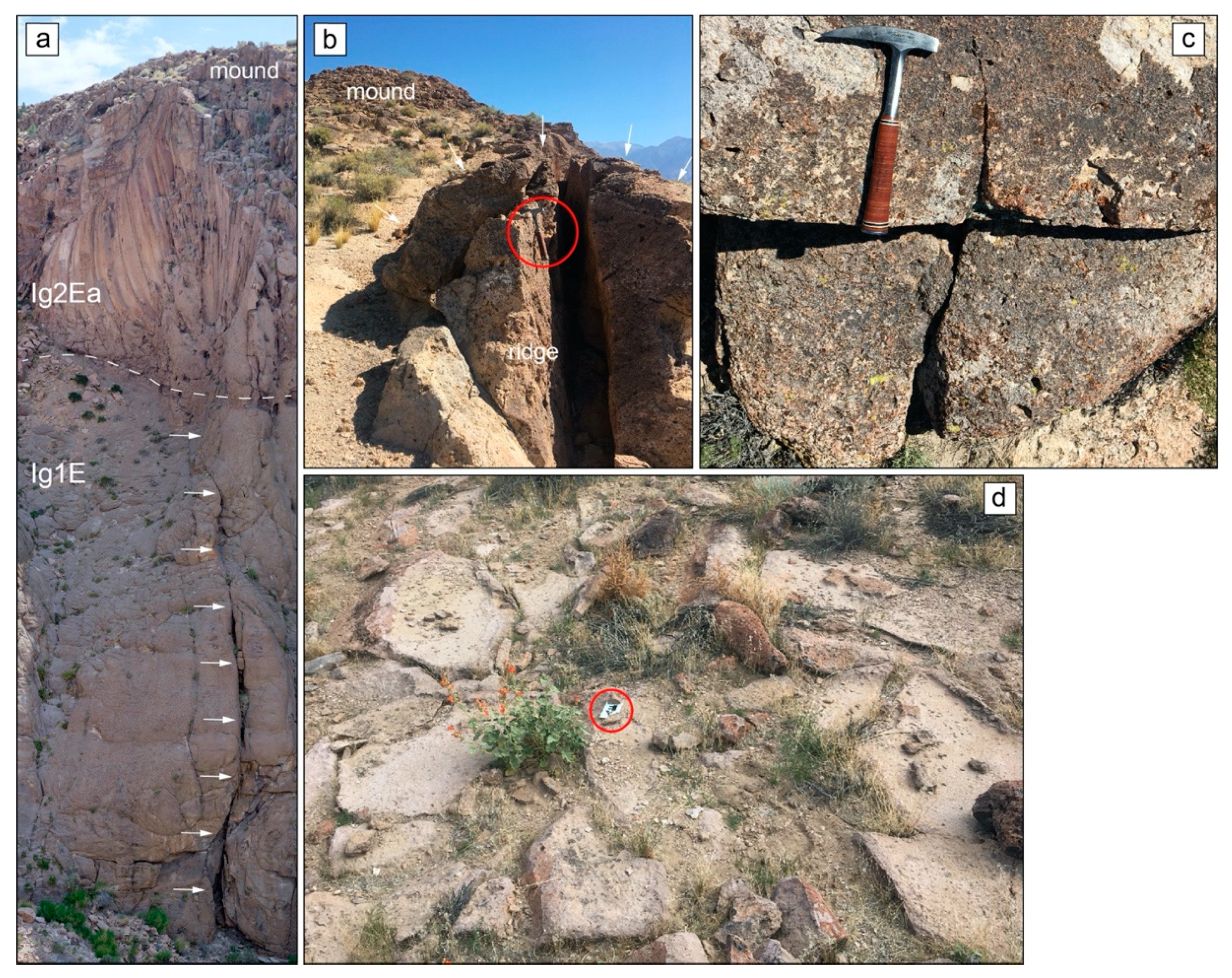
3.1.2. Fault Exposures

Our field efforts resulted in the discovery of 31 well-preserved fault localities showing in situ fault planes and slickenlines that have not been described in previous research on the Volcanic Tableland. These localities are distributed across the field site (Figure 2 and Figure S1), and each contains many distinct fault surfaces for analysis. The morphology for each of these newly identified fault surfaces varied according to their corresponding emplacement subunit. We note that the scale of the majority of the fault surfaces described here is below the scales of the previous maps, and the numbers of localities and slickenline measurements are small relative to the total number of fault scarps in the tableland, but their characterizations provide valuable information of the fault geometry and fault slip.

In the northern half of the tableland, where non-welded Ig2Ea and Ig2Ec are exposed at the surface, nearly all fault surface exposures were found in the upper half of the talus piles that were deposited on the hanging walls as a result of the toppling of cooling-joint bounded columns. Erosion and sedimentation have obscured or destroyed many of the original fault surfaces (images 4 and 5 in Figure S1) in the non-welded tuff, and the remaining exposures are often on the order of centimeters to meters in scale, however the largest continuous fault surface discovered in this area was ~235 m long and 1−2 m tall (image 6 in Figure S1). Fault surfaces are indurated relative to tuff in their immediate vicinity, which is a function of minor gouge formation along the slip surface and/or case-hardening from thin mineralized coatings of iron oxides that stain the surface orange and brown. Desert varnish is also present on some exposures. A typical fault surface in this area of the tableland exhibits grooves and slickenlines in white caliche encrustations (Figure 5). Some fault surfaces even display a displaced soil profile indicative of relatively recent deformation (image 7 in Figure S1).

In the southern half of the tableland, fault surfaces are preserved along reactivated joint faces (cm to m in scale) in moderately to densely welded (Ig2Eb) tuff. Mapped faults in this area are subparallel with the strike of existing conjugate joints or curve to intersect conjugate joints near their tips. This indicates that faulting utilized preexisting structural weaknesses in the ash-flow sheet. Furthermore, mapped fault traces vary from having a single isolated scarp to an anastomosing arrangement of scarps. On a finer scale, fault scarps display a similar pattern whereby their trace follows the preexisting structural fabric of the jointed rock mass. Fault surfaces were discovered where jointing (conjugate or cooling) approaches parallelism with fault strike, allowing for shear to occur along joint planes. Given this mechanism, the fault surfaces in this area are frequently vertical to sub-vertical (image 8 in Figure S1) according to the orientation of the preceding joint. Interestingly, previously analyzed displacement profiles of faults that tip-out into these conjugate joints are found to typically show a decrease of the displacement gradient where the fault tip has propagated along a preexisting joint [38].

As exposed tuff in this area is moderately to densely welded, fault surfaces are predominantly grooved and show little evidence of fault gouge. Slickenlines are present where caliche has been deposited from fracture flow occurring along fault and joint surfaces. Furthermore, sinistral horizontal chatter marks were observed at one outcrop in the field (image 9 in Figure S1), although they are not a common feature of fault surfaces in the area.

Across the field site, normal and oblique faults (Figure 5a,b) are more numerous and larger in scale than faults classified as being strike-slip. Normal and oblique faults have notable vertical offsets ranging from 1 to 145 m and preserve large footwall scarps. Lateral offsets along strike-slip faults, however, were not visible in the field due to the poor outcrop of fault traces along the surface of the tableland, which are likely buried beneath loose sediment. Likewise, the homogenous composition and appearance of the tuff precludes identifying any offset in lithology. We also did not identify strike-slip surfaces (Figure 5c) where both fault walls were preserved. Thus, all strike-slip fault surfaces were discovered where one side of the fault had been exposed by erosion, collapse of one fault wall, or minor oblique offset from a shallowly plunging slip vector.

Along fault planes but also on joint surfaces or loose cobbles, caliche commonly coats the fracture surfaces (image 10 in Figure S1). It forms a variety of textures ranging from coralloidal, botryoidal, dendritic, to laminar, which all appear to be a function of available void space and deposition mechanism. We observe it most commonly to be laminar, apparent as thin coats of rounded lithics bound in calcareous cement (image 11 in Figure S1). This laminar texture indicates that meteoric water played a role in transporting the caliche constituents along these fault and fracture planes. Due to its pervasive nature, slickenlines are frequently preserved in caliche along fault surfaces. We find that preservation of slickenlines is enhanced when a coating of caliche is developed on a fracture plane, but the presence of caliche is not a prerequisite for the preservation of fault kinematic indicators. The relative timing and deposition of caliche with regards to faulting is variable across the field site, whereby some non-mineralized fault grooves are coated by undeformed caliche and some fault surfaces display slickenlines in the caliche itself. In fact, some structural overprinting of slickenlines was observed along fault surfaces where caliche was deposited laminarly, thereby preserving two distinguishable fault slip directions in separate laminations of caliche (Figure 5d).

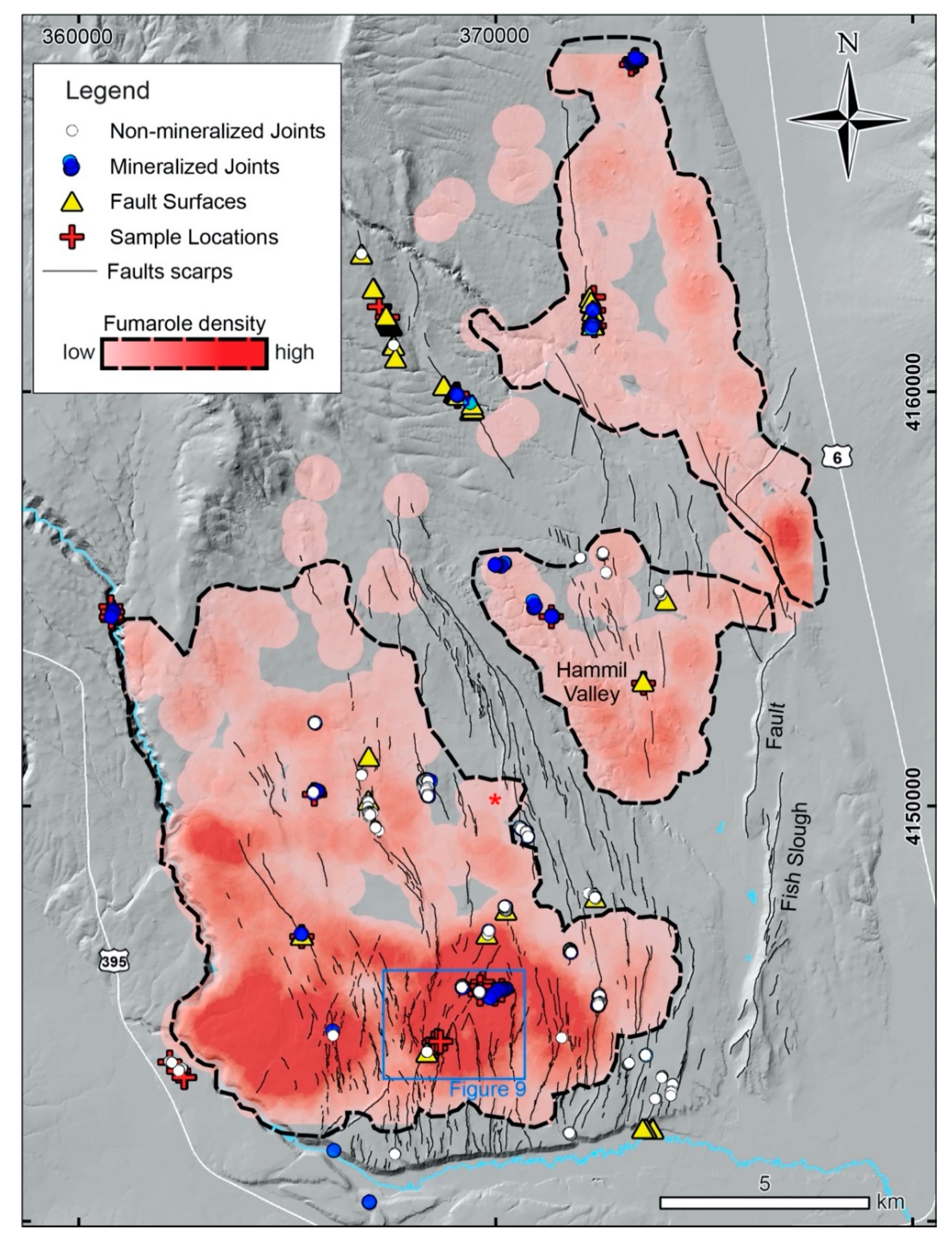
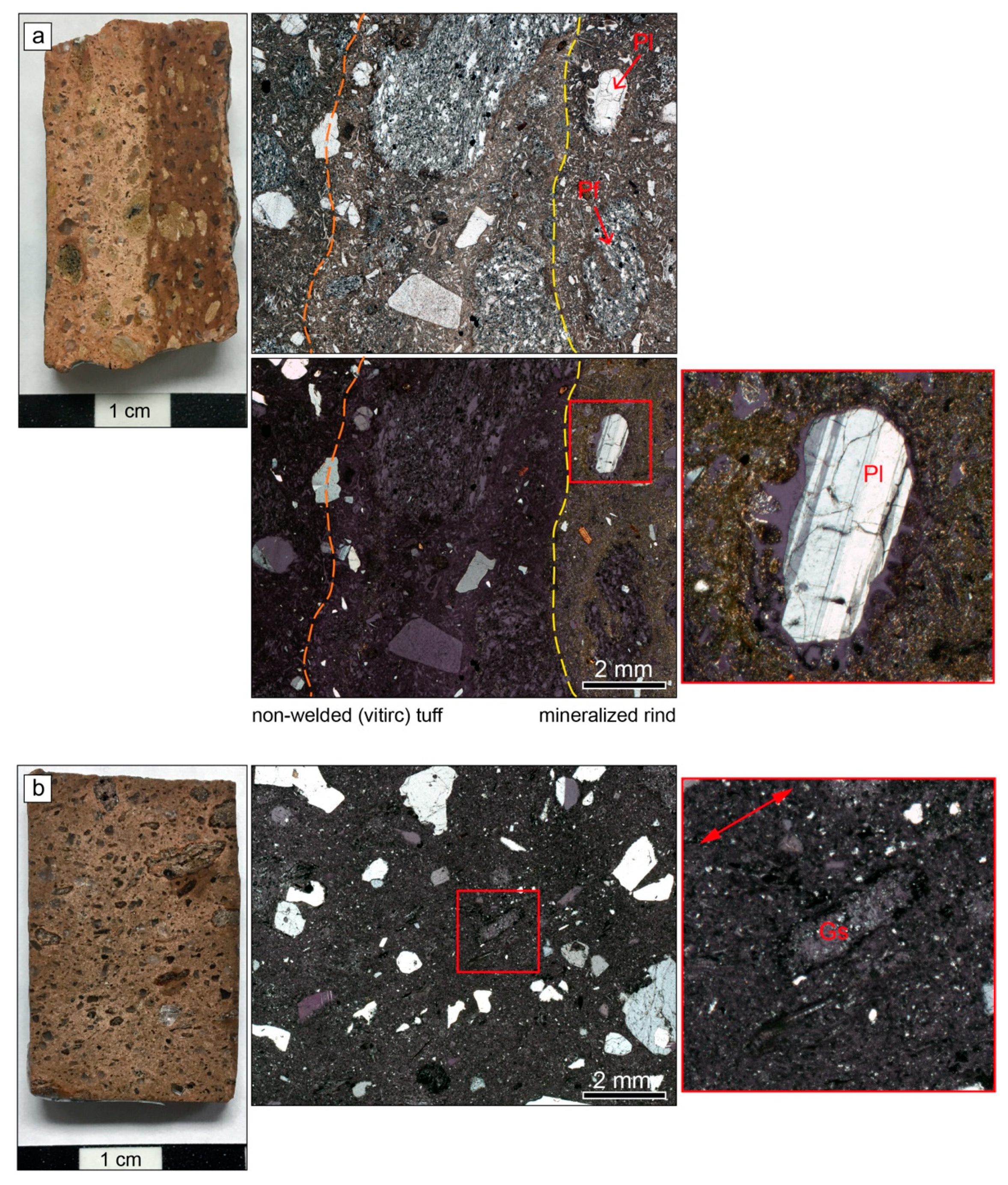
3.2. Hydrothermal Mineralization of the Bishop Tuff

Vapor-phase alteration caused by fumarolic activity notably changed the mineral grains and tuff matrix at both macroscopic and microscopic levels. The alteration occurred within the tuff along surfaces that came in contact with fumarolic vapors and/or vapor condensate forming an indurated rind. This process made the tuff more resistant to erosion as compared to its unaltered, unwelded, and thus, friable counterparts, preserving evidence of fumarolic activity in the form of mounds and ridges (Figure 6). The rinds represent where the vitric tuff matrix has been replaced with microcrystalline quartz, that, when broken, produces a conchoidal fracture similar to chert or jasper. Fumarolic rinds are commonly ~10 mm or less in thickness (Figure 7a, image 1 in Figure S1), but, in places, thicker rinds can be observed in the field. Most of the fumarolic alteration is light to dark gray with lesser amounts of pale pink, blue, or red.

In thin section, vapor-phase alteration is apparent where the vitric matrix of the tuff has been replaced with birefringent microcrystalline quartz, filling the void space in the tuff matrix and defining a distinct contact (Figure 7a). As samples were collected from the surface of the tableland, where fumarolic alteration affected non-welded tuff, the original vitric texture (non-welded cuspate glass shards) is frequently preserved in these rinds with microcrystalline quartz preferentially altering the fine-grained ash matrix. Some larger mineral grains in silicified rinds have developed haloes of recrystallized glass or quartz (Figure 7a). Furthermore, a “bleached” zone is commonly observed along the contact between this silicified rind and the unaltered tuff, where the vitric matrix appears to be lighter than the adjoining matrix but does not display the same microcrystalline alteration as the rind (Figure 7a). The nature of this alteration type is found to be representative across all sites of vapor-phase alteration on the Volcanic Tableland.

Zones of vapor-phase alteration are found to overlie the welded and devitrified lower emplacement unit of the Bishop Tuff (Ig1E), which we also sampled for petrographic analysis. These zones were formed from volatiles released during the devitrification of Ig1E, as SiO₂ and anhydrous feldspars formed from glass present in the hot ash and pumice of the ignimbrite [16]. As a result of devitrification, water and other volatiles present in the volcanic glass were released in the vapor-phase which, coupled with the residual heat of the ignimbrite and likely addition of meteoric and/or hydrothermal water, fueled fumarolic activity and vapor-phase alteration in the tuff [17].

In thin section, welding is readily identified by the flattening and alignment of mineral grains, pumice clasts, and glass shards (Figure 7b). Devitrification is identified where glass shards and volcanic ash have been notably replaced by quartz (SiO₂) +/− anhydrous feldspar. This recrystallization is best described as fine-grained axiolitic and spherulitic mineral growths extending inward from shard walls (Figure 7b).

3.3. Structural Analysis

3.3.1. Fault Analysis

Measurements of slickenlines and their corresponding fault surfaces allow us to carry out a kinematic analysis of the fault slip, which is important for understanding the relationship of faults in the tuff with those present in the surrounding or underlying rock volume. The orientations of 267 slickenline measurements and corresponding fault surfaces were recorded from 31 fault localities for structural analysis (Figure 8). To analyze this fault data, we imported our measurements into Allmendinger’s FaultKin software [37]. Kinematic analysis of our fault-slip data was performed [39] by calculating the kinematic axes (P and T) of each recorded slickenline and fault plane pair. This allowed us to classify each fault and calculate averages for each fault type. Faults were classified into dip-slip, oblique-slip, and strike-slip faults using a simplified version of the Zoback criteria whereby faults were grouped by the plunge of their respective kinematic axes to identify their stress regime: normal fault (P plunge > 52°, T plunge < 40°), oblique fault (40° < P plunge < 52°, T plunge < 40°), and strike-slip fault (P plunge < 40°, T plunge < 40°) [40,41]. Following these criteria, 197 of the recorded faults were dip-slip, 49 were oblique-slip, and 21 were strike-slip. However, structural overprinting was observed along several fault surfaces (Figure 5d) such that these fault planes fell int two different categories. The orientation of slickenlines and grooves was dependent upon fault type, and plunges varied between 0° and 88° depending upon fault dip.

Stereonet plots showing fault planes, striae, and slip-sense, are presented in Figure 8. Stereonets were plotted to display all collected data (Figure 8a) as well as the previously classified fault types. Normal faults (n = 197) have an average strike of 157° and dip between 53° and 87° (averaging ~ 65°) slightly to the southwest and northeast. In total, 188 of these fault surfaces are west-dipping and 9 are east-dipping (Figure 8b). Based on the geomorphology of the fault scarps, Ferrill et al. [26,27] report an approximate equal number of east-, and west-dipping faults in the area. We agree with this assessment and note that our data report fault planes with preserved slickenlines, which were found more frequently on west-dipping faults. The average orientation of striae on these dip-slip surfaces has a trend of 243° and plunge of ~64°, which translates to a rake of 88° for the average fault plane orientation. Faults identified as displaying strike-slip kinematics (n = 21) have two modes with average strikes of 223° and 330°. Their dips range from 73° to 89°, averaging 82° and 86°, respectively. In total, 16 fault surfaces are west-dipping and 5 are east-dipping. Striae along strike-slip faults have trends nearly parallel to strike and an average plunge of 16°. Striae along northwest-striking faults plunge shallowly to the northwest and southeast, while striae on northeast-striking faults plunge shallowly to the northeast and southwest (Figure 8c). Faults identified as exhibiting oblique-slip (n = 49) display two modes with average strikes of 152° and 211°. Their dips are between 77° and 89°, averaging ~ 85°. In total, 42 of these fault surfaces are west-dipping and 7 are east-dipping. Striae on these fault surfaces have variable trends and an average plunge of ~75° (Figure 8d).

The kinematic data were analyzed using the stress analysis module in the Move2018 software to calculate the orientations of the principal stress axes associated with the faulting observed in the field. This stress analysis module is based on the method by Angelier [42] and assumes that slickenlines contained within a fault plane represent the direction of maximum shear. The minimum principal stress axis (σ₃) was used to determine the direction of extension for the field site, and the direction of the intermediate principal stress axis (σ₂) was compared for parallelism with recorded fault strikes in accordance with the Andersonian fault theory [43].

The data show that normal and oblique faulting display a sub-vertical maximum principal stress component (σ₁), trending 75° and plunging 79°. The minimum principal stress component (σ₃) is sub-horizontal, trending 256° and plunging 11°, and its axis is parallel to ENE and WSW extension. The intermediate principal stress (σ₂) is horizontal and trends 346°, roughly parallel with the average strike of 159° of the recorded normal and oblique faults (Figure 8b,d). Stress inversion was also performed using the 21 recorded strike-slip faults and lineations (Figure 8c). The resulting maximum principal stress axis (σ₁) is horizontal and bisects the conjugate NE and NW strike-slip fault planes, trending 12°. Similarly, the minimum principal stress axis (σ₃) is horizontal and its axis parallels lateral ESE and WNW extension, trending 102° and plunging less than 3°. The intermediate principal stress (σ₂) is near-vertical, trending 281° and plunging 87°.

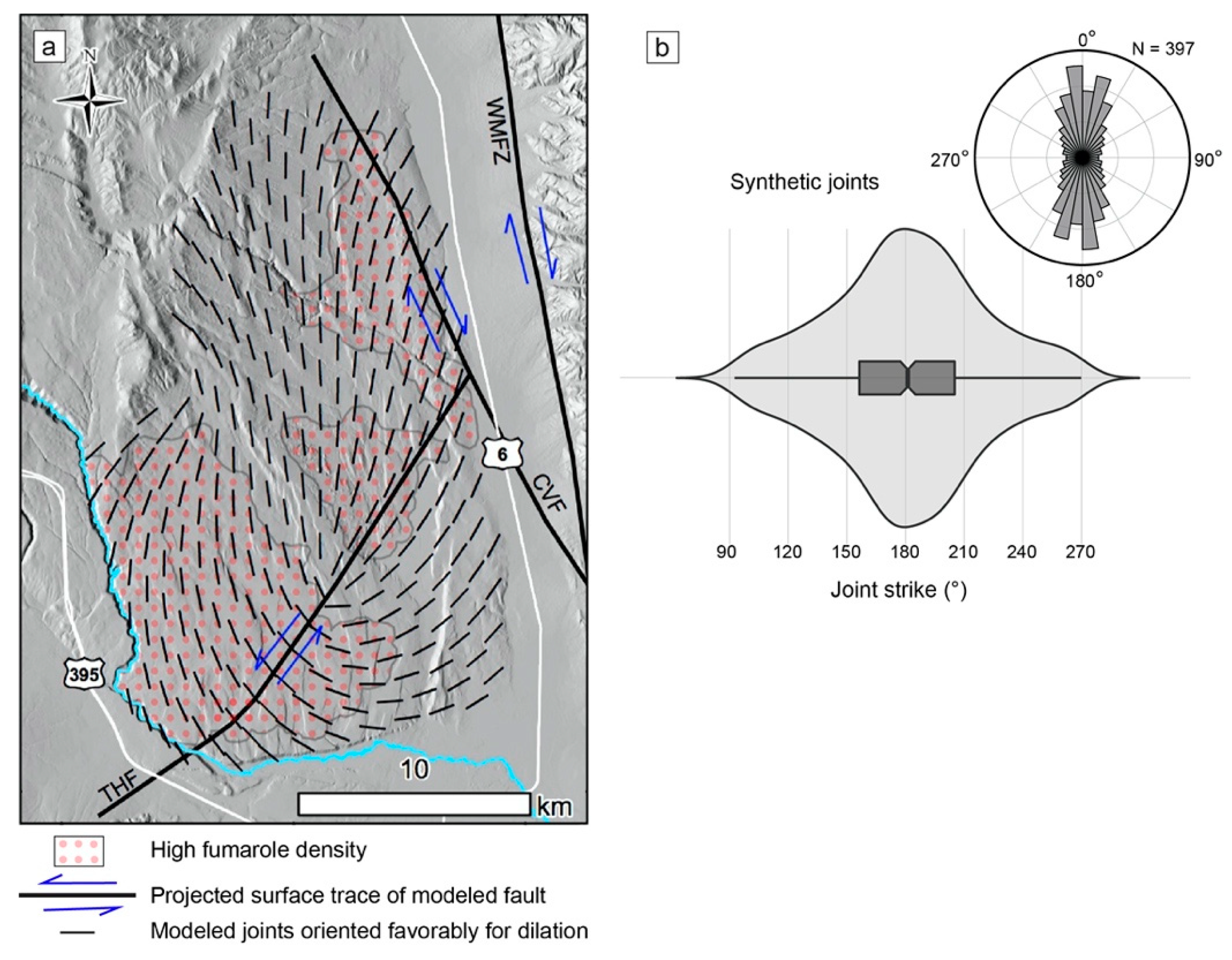
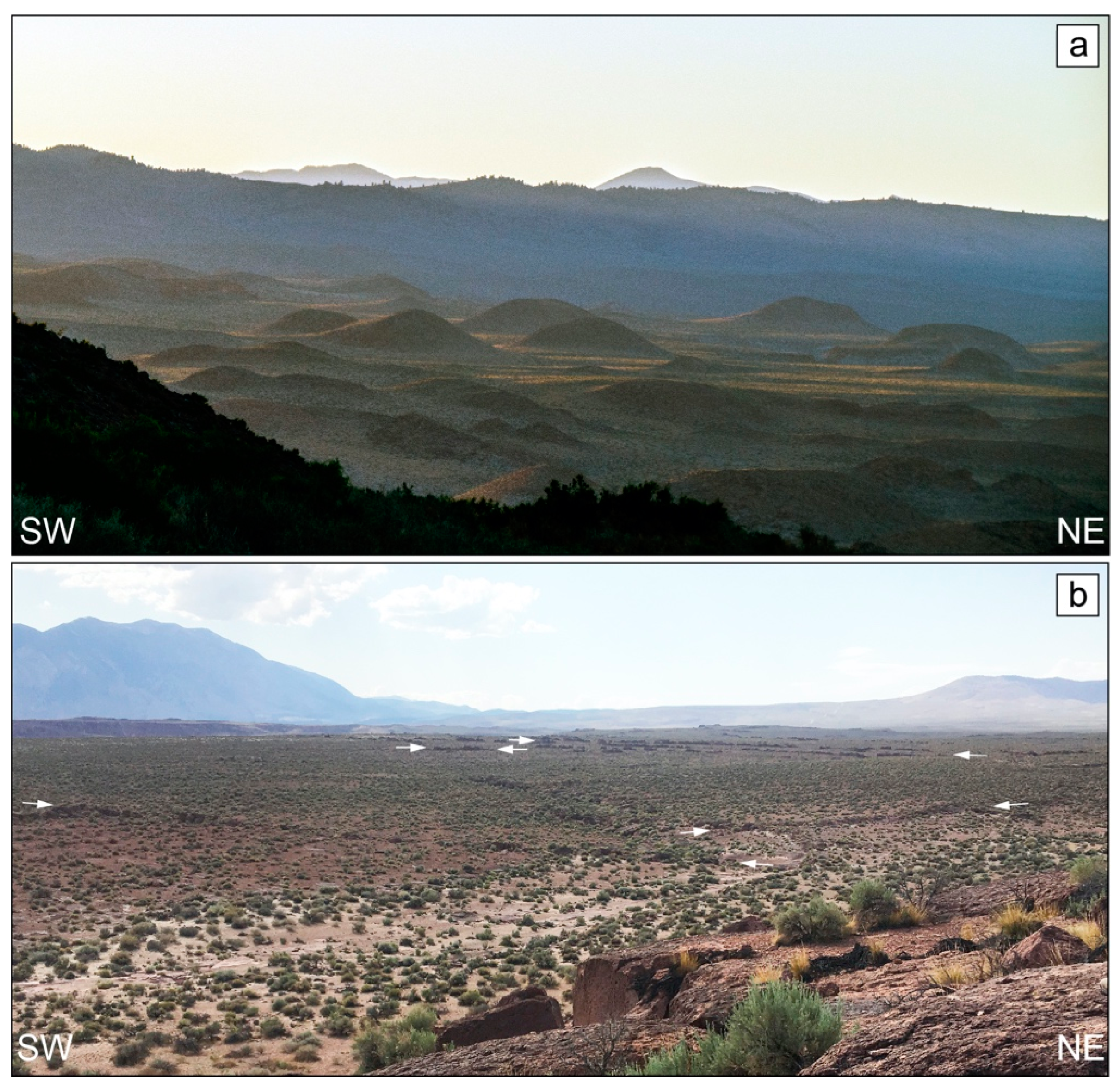
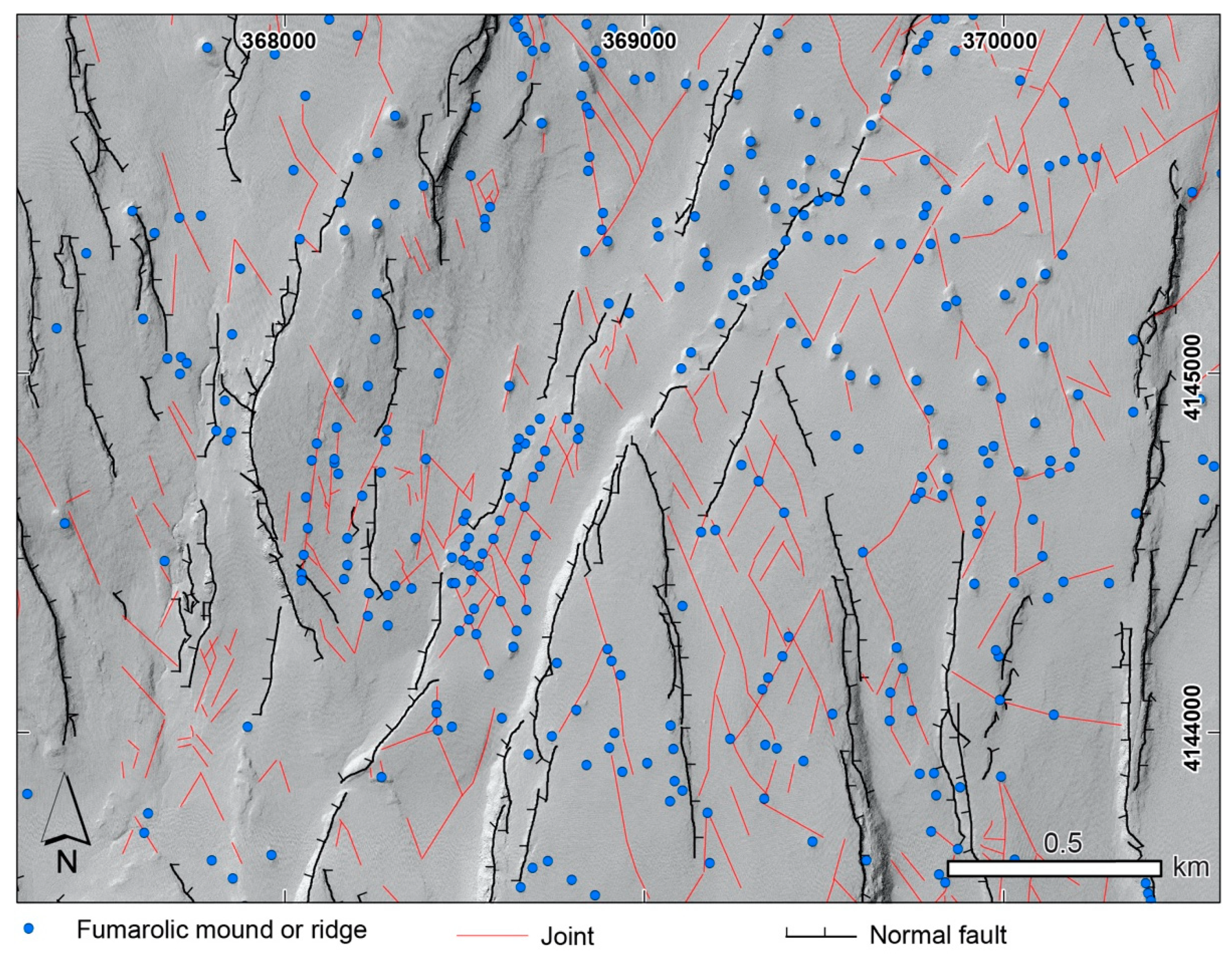
3.3.2. Spatial Relationships of Fumarolic Landforms with the Fracture Network

We find evidence of vapor-phase alteration to be present along what we interpret as preexisting or coeval discontinuities of variable scales. Because we observe hundreds of mineralized joint planes, it is very likely that vapor-phase activity was directed to the surface of the Volcanic Tableland via an extensive network of joints. In the immediate vicinity of fumarolic mounds and ridges, structures of all scales (including small polygonal cooling cracks) may be mineralized (Figure 3), and many of these structures have a lighter halo of vapor-phase alteration around their circumference.

We assessed the spatial relationship between fumarolic features and discontinuities using ESRI’s ArcGIS and the R software. We mapped 1214 fumarolic mounds and ridges apparent on 1-meter resolution aerial images and DEMs, and analyzed their locations with respect to our mapped to faults (491) and joints (1339) within the same extent of 1-meter resolution data. An exemplary map of the fracture network and locations of fumarolic landforms in an area of high fumarole density is shown in Figure 9. The Near tool in ArcGIS was used to calculate the nearest distance between fumarolic mounds and discontinuities (faults and joints), and a spreadsheet of fumarolic attributes (coordinates and nearest distance to discontinuity) was exported for analysis in R. These attributes were compared against a population of 50,000 randomly distributed points (UTM coordinates) generated in R that fell within the same extent of 1-meter resolution data. The randomly generated coordinates were imported into ArcGIS as point features, and the Near tool was used again to calculate the nearest distance between the randomly distributed points and discontinuities. A bootstrap function was written in R to sample “near” distances from the randomly generated points and calculate a mean of that sample. This sampling was performed with replacement, and sampling size was limited to the total number of observed fumarolic mounds in the 1-meter data resolution extent (1214). This process was repeated for a total of 10,000 replications, generating a total of 10,000 mean distances to a discontinuity from the resampling of randomly located points. From this normal distribution, 95% confidence limits were calculated to obtain an estimate of the mean distances to a discontinuity provided the fumarolic mounds were randomly located across the ash-flow sheet. The results of this bootstrap were compared to the mean distance from the observed fumarolic mounds to a discontinuity to analyze whether the observed fumarolic mounds followed a random distribution.

Our results indicate that, on average, the observed fumarolic mounds are 30.59 m from a discontinuity. Whereas, the mean distance from a random point to a discontinuity is 70.86 m, yielding a difference in mean distances between the observed fumarolic mounds and the randomly generated points of 40.27 m. Additionally, the 95% confidence interval generated from the normal distribution of bootstrapped means yields confidence limits of 66.47 to 75.50 m to a discontinuity from a randomly located point; thus, the mean distance to a discontinuity from the observed fumarolic mounds is not captured within the confidence interval. Therefore, for randomly distributed points, the probability of calculating a mean distance that is similar to that of the observed fumarolic mounds is significantly less than 5%. This suggests that fumarolic mounds in the Bishop Tuff are not randomly distributed, indicating that a spatial relationship exists between fumarolic mounds and discontinuities. This relationship suggests that the migration of vapors within the ash-flow sheet was anisotropic. In such extensive fracture network, most vapors readily utilized the nearest vertical fractures to escape toward the surface, but, in cases where no vertical conduit was nearby, some lateral migration of vapor toward a vertical conduit in a diffuse manner cannot be ruled out. Such findings are in accordance with previous field observations of the area and support the suggested sequence of events whereby fumaroles were produced at the surface after the formation of fractures in the ash-flow sheet [16,18].

To better understand the spatial density of fumarolic features across the tableland, we used the Point Density tool in ArcGIS to analyze the entirety of our mapped fumarolic features (2, 164). The resulting map shows the density of fumarolic structures, calculated for a point density sample radius of 500 m, concentrated in three regions (Figure 2) highlighting a clear relationship between fumarolic landforms and conjugate joints and faults throughout the southern half of the tableland, where Ig2Eb forms a densely welded cap. Fumarolic mounds and ridges are frequently aligned in preferred northeast and northwest trends along the strike and intersections of conjugate joints (Figure 9). In several areas, fumarolic mounds are aligned along fault lines and have been cut by subsequent faulting events (images 2 and 12 in Figure S1), indicating that faults were also capable of vertically communicating fumarolic vapors and that faulting occurred while hydrothermal activity was ongoing but also continued after fumarolic activity ceased. In the northern half of the field site, however, the relationship between joints or faults and the fumarolic landforms becomes less apparent in aerial imagery, as the friable non-welded Ig2Ea and Ig2Ec units have eroded so much as to obscure the structures that once served as pathways for fumarolic vapors. However, our field observations confirm that fossil fumarolic features in this area are still related to joints and faults in the tuff, as is indicated by the presence of alterations along structures, thus this relationship appears to be ubiquitous across the field site.

One location where fumarolic alterations occur along irregular and curvilinear cooling joints (instead of conjugate joints or faults) is found in an area north of Casa Diablo road near the coordinates 370,000 m E and 4,140,000 m N (red asterisk in Figure 2). The area is located on the margin of a buried basin identified by gravity surveys [7,44]. Here, fumarolic ridges resemble a curvilinear latticework along connected traces of cooling joints. Alteration along these curvilinear fumarolic ridges bears all the same characteristics as fumarolic features found elsewhere in the field site, with a silicified rind indurating the ridges relative to the surrounding tuff.

3.4. Fracture Dilation in the Bishop Tuff in Response to Regional Faulting

We model the stress field around regional faults to test if tectonic activity played a role in enhancing joints in the Bishop Tuff as pathways for hydrothermal fluids. The Move2018 software was used to plot earthquake hypocenters of the 1986 Chalfant Valley Earthquake Sequence from the Northern California Earthquake Data Center and interpolate large-scale regional fault planes beneath the Volcanic Tableland to form a three-dimensional fault model, similar to methods in previous studies [21,29]. In particular, Smith and Priestley [29] identified three fault planes active during the earthquake sequence from relocated aftershocks, depicting a conjugate strike-slip system consisting of the Chalfant Valley Fault (CVF) and Tungsten Hills Fault (THF) and the White Mountain Fault Zone (WMFZ). These fault planes were easily identified by the geometry of their hypocenters, with Y-junctions apparent between the CVF-THF and the CVF-WMFZ. This allowed for the isolation of hypocenter point clouds for each individual fault plane, from which three-dimensional fault surfaces could be interpolated using Inverse Distance Weighting (Figure 10). The interpolation produced average orientations for the THF striking 220°, dipping 55°, CVF striking 153° and dipping 45°, and the WMFZ striking 170°, dipping 70°, yielding close matches to the preferred fault planes for solutions to short-period focal mechanisms of three analyzed events in Smith and Priestley [29].

As the modeled conjugate strike-slip system has not been observed to break the surface of the tableland, it was constrained vertically by the maximum and minimum depths for hypocenters on each plane. The WMFZ, however, is manifested along the intersection of the Owens Valley floor and base of the White Mountains. Therefore, the upper limit of the fault plane was modeled according to its surface expression, and the lower limit was constrained by its respective maximum hypocenter depths. The interpolated surface was extended along its strike according to its mapped trace along the base of the White Mountains [18]. After each fault surface was interpolated from its respective hypocenter point cloud, a smoothing tool was used to eliminate computer-generated asperities and create more realistic fault surfaces (Figure 10).

In order to simulate the stresses that were active during the 1986 Chalfant Valley Earthquake Sequence, Move’s Fault Response Modeling module was used to assign displacement magnitudes and directions along the three interpolated fault surfaces and stress, strain, and displacement around the fault planes in an elastic medium were modeled. For the purpose of this study, the observational surface was created in Move2018 to represent the current expression of the Bishop Tuff atop the Volcanic Tableland at an average elevation of 1500 m above sea level. Since fault slip is not uniform across a fault plane, slip maxima were defined in the centroid of each modeled fault and slip was tapered toward the fault tips, represented in Figure 10 by a gradational color scheme. Likewise, given that faulting does not occur in an infinite elastic medium, a free surface was defined directly above the modeled elevation of the Bishop Tuff in order to accurately model elastic dislocations in a half space [45]. The elastic halfspace in Move’s Fault Response Modeling module does not capture any heterogeneities within the modeled domain including the rheologic differences that may exist between the Bishop Tuff, the unconsolidated Owens Valley basin fill, and the Owens Valley basin floor, but, assuming that stresses are nevertheless communicated throughout these units, it is applicable for resolving stresses acting on predefined fracture planes providing insights into the response of such fractures to the modeled faulting.

In accordance with previous studies, the slip senses on the CVF and WMFZ were assigned to be dextral, and the THF to be sinistral [29,33,36], however, we note that some dip-slip component along the THF potentially contributed to the topographic relief in the Tungsten Hills. Stress drop and displacement calculations by Smith and Priestley [29] yielded average slip displacements of 1.50 m on CVF, 0.71 m along the THF, and 0.25 m along the WMFZ. As there are no observations to support modeling any opening or closing that occurred along the full extent of each fault surface, such parameters were omitted from the simulation. Our model assumes that the kinematics of the faults displayed during the 1986 Chalfant Valley Earthquake Sequence are representative of their long-term slip, as their overall kinematics are compatible with GPS-derived deformation fields (e.g., [46,47]). Other major faults in the region, such as the Sierra Nevada range front or Owens Valley faults, likely also have an impact on the orientations of joint dilation but for simplicity and because they are outside the domain of our model, they were not included in this study.

From the simulated the stress field (Table S3), a set of synthetic joints (n = 397) taken to represent fumarolic pathways was extracted. Joints within the set were chosen at an equal spacing of 1.5 km across the 350 km² extent of the field site (Figure 11). This sample size was selected in order to match the number of recorded mineralized joints in the field. Although a smaller joint spacing would yield a greater number of synthetic joints, the distribution of joint orientations would remain the same given they are a function of the reproduced stress field. The synthetic joints were assigned a vertical dip and a length of 500 m in order to reflect the vertical nature of fumarolic pathways observed in our field data and in previous research [16,18]. To find the optimal azimuth of a synthetic joint, the software rotated the azimuth of each joint plane in 1° intervals around a full 360° and selected the azimuth with the maximum Coulomb stress change according to the chosen displacement, in our case dilation. The model output produced a synthetic fracture network (Figure 11a) that was most likely to experience dilation given the stress conditions exhibited during the 1986 Chalfant Valley earthquake sequence. This synthetic joint network displays a pattern that is influenced by all three faults of the conjugate strike-slip system. Joints likely to experience dilation display high angles with respect to the NW portion of the projected CVF, are perpendicular to the projected THF trace in its SW portion, but are sub-parallel to the projected THF trace in its NE portion (Figure 11a). The CVF was the dominant fault of the fault system during the 1986 Chalfant Valley earthquake sequence, and thus it influenced joint dilation even in parts of the Bishop Tuff that directly overlie other faults, such as the THF.

Figure 11. Model output of joints oriented optimally for dilation. (a) Map showing joint orientations and the surface projections of the three fault surfaces with respect to areas of highest fumarole density. The sense of slip along each fault plane is indicated with blue arrows according to the motion described by Smith and Priestly [29]. (b) Modeled joints oriented optimally for dilation show a bimodal distribution of NE- and NW-striking orientations with an average optimal strike of 181°. The probability density function of the synthetic joints is distributed such that there is a sharp increase in the likelihood strike values between 150° and 210°. Note the similarity of modeled violin and rose plots to that of the mineralized joints recorded in the field (Figure 4b).

Figure 11. Model output of joints oriented optimally for dilation. (a) Map showing joint orientations and the surface projections of the three fault surfaces with respect to areas of highest fumarole density. The sense of slip along each fault plane is indicated with blue arrows according to the motion described by Smith and Priestly [29]. (b) Modeled joints oriented optimally for dilation show a bimodal distribution of NE- and NW-striking orientations with an average optimal strike of 181°. The probability density function of the synthetic joints is distributed such that there is a sharp increase in the likelihood strike values between 150° and 210°. Note the similarity of modeled violin and rose plots to that of the mineralized joints recorded in the field (Figure 4b).

The model output allows us to compare synthetic joint orientations with the observed orientations of fumarolic pathways. For our simulated stresses, synthetic joints oriented optimally for dilation show a bimodal distribution of NE- and NW-striking orientations (Figure 11b) with an average optimal strike of 181°. The probability density function of the synthetic joints is distributed such that there is a sharp increase in the likelihood of strike values between 330° and 30° or 150° and 210° (Figure 11b). These values do not show any noticeable similarities to orientations of the non-mineralized joints (Figure 4a), but compare well to the orientations of mineralized joints recorded in the field (Figure 4b), which have an average strike of 2° and an increased likelihood of striking between 330° and 30°. Furthermore, the synthetic joints are bisected by σ₁ generated from the stress inversion of strike-slip fault surfaces observed in the field (Figure 8c). These findings indicate that the synthetic joint set shows similar orientations as the set of mineralized joints observed in the field, and that joints of those orientations are compatible with the kinematic record of strike-slip faulting preserved in the Bishop Tuff. Minor differences between the observed and synthetic joint orientations are attributed to natural variations in the recorded field data, differences in data sampling between the model and field work, and the resolution of our model. Yet, the close match between synthetic and observed, mineralized joints shows that the kinematics of the conjugate strike-slip system displayed during the 1986 Chalfant Valley Earthquake Sequence alone are able to explain joint dilations, corroborating that regional deformation is represented sufficiently by the earthquake sequence and that other faults outside our model domain likely only had minor impacts on joint dilation in the Bishop Tuff.

4. Discussion

The Bishop Tuff contains exposures of fault surfaces that serve as kinematic indicators. We collected measurements of a total of 267 slickenline and fault plane pairs, of which 21 (8%) and 49 (18%) pairs are indicative of strike-slip and oblique slip fault kinematics, respectively. These observations are consistent with the kinematics of the buried strike-slip fault system involved in the 1986 Chalfant Valley Earthquake Sequence [29], suggesting that the strike-slip tectonics at depth are also expressed in the Bishop Tuff. Considering that normal faulting is the most frequently observed type of faulting, it is possible that the geometry of the strike-slip fault system at depth promoted the formation of a negative flower structure whereby faults at the surface would predominantly display normal displacements.

Fracture dilation modeling that was informed by these field observations and earthquakes suggests that hydrothermal fluids circulated through the fracture network of the Bishop Tuff in a systematic manner, causing mineralizations and hydrothermal alterations that are manifest as mounds and ridges to be collocated with or near joints and faults, showing a dense geographic clustering in three areas. Together, these findings have general implications for fluid migration in fracture networks, and are important for the origin of hydrothermal fluids, as well as the formation and localization of fumaroles in the Bishop Tuff in particular.

Conjugate joints in the Bishop Tuff are evident across the Volcanic Tableland. The formation of these joints are suggested to have involved shear [10,16], although the mechanisms for their formation have not been explored in great detail. Bateman [10] suggests that the fractures represent conjugate shear planes formed from a regional horizontal principal stress, similar to the conjugate structures observed in the nearby Sierra Nevada and Tungsten Hills. Our stress inversion analysis supports this conclusion of Bateman [10], as maximum horizontal stresses in solutions of stress states from our fault measurements bisect the acute dihedral angle between mineralized conjugate fractures and conjugate strike-slip faults recorded in the field. This suggests that a N−S horizontally oriented maximum principal stress component is kinematically compatible with conjugate fracture orientations, conjugate strike-slip faults observed at the surface, and the blind conjugate strike-slip zones at depth, implying that the regional tectonic stress field caused the formation of the conjugate fractures. Furthermore, the orientation of the minimum horizontal stress for all faults observed in the field supports E−W extension and the development of NE to NW striking opening-mode joints between azimuths of 348° and 12°.

If the conjugate fractures were some of the first discontinuities to develop after welding in the Bishop Tuff, as has been suggested [10,16,18], then they may represent precursors to fault development on the tableland. Their similarities to the orientations of strike-slip surfaces, their vertical continuity (Figure 3a), and the fact that many faults have preferentially propagated along the strike of conjugate fractures support this finding. Furthermore, this has implications for the paleostress regime around the time that the Bishop Tuff was emplaced. If conjugate fractures developed soon after tuff emplacement but are consistent with the tectonic regime of the strike-slip derived from the 1986 Chalfant Valley earthquake sequence, then these strike-slip tectonics must have operated already at the time of the tuff emplacement.

Findings on the orientations and alteration of conjugate joint planes indicate that they constituted the primary pathways for fumaroles on the tableland (see Section 3.3.2) [10,16,18]. Our field observations indicate that fumarolic activity also occurred along polygonal cooling cracks in areas immediately adjoining fumarolic features, and that cooling joints form curvilinear ridges on the distal and shallow margins of buried basins. These structures likely account for some of the variability of the orientations of altered joints (Figure 4b) as compared to the modeled joints (Figure 11b).

Fumarolic activity of the tableland is found to have formed from gases and/or vapors and latent heat derived mostly, if not entirely, from the welding and devitrification of the cooling ash-flow sheet [16,17,18,48,49]. Therefore, the mapped distributions of the three fumarolic zones of the tableland correspond to the degree of welding and devitrification in the Bishop Tuff [6,8]. However, given the location of the tableland on the flanks of the Long Valley Caldera, volcanism in Owens Valley proper as recent as 17 ka [50], and hydrothermal activity on the valley floor along deep, valley-bounding faults, including the Fish Slough Fault thermal springs, Keough’s Hot Springs, and Benton Hot Springs, there is reasonable potential for an additional source of hydrothermal fluids or perhaps fault-valve activity from ascending overpressured fluids [51] to have supported fumarolic activity.

There are currently three active thermal springs emerging from NE-striking fault tips on the Fish Slough Fault in an area with extensive vapor-phase alteration and fumarolic features. Jaykoh and Fatooh [34] note that these springs are likely rooted to a deeper hydrothermal system, and that the area’s water table rose as a result of the 1986 Chalfant Valley earthquake sequence. The duration of this rising water table peaked approximately one year after seismic activity, and tapered to preexisting levels approximately six years later [34]. This indicates that it is a structurally enhanced system, where short term water-level rises following seismic activity are related to compaction and reduced permeability. As the Fish Slough Fault has been interpreted to root into the pre-Cenozoic basement [7,10,44,52], it is likely that it taps into a deep hydrothermal system located beneath the Bishop Basin. Furthermore, meteoric water present at the time of, and following, the tuff emplacement may have played some additional role as a source of the fumaroles. Holt and Taylor [18] suggest that the hydrothermal circulation of meteoric water through the cooling tuff would serve as an additional source for fumarolic vapors, while simultaneously accounting for the lack of deeper hydrothermal signatures observed in the fumarolically altered tuff.

Despite these potential secondary sources, we only identify microcrystalline quartz and minor amounts of K-feldspar in our petrographic analysis of the fumarolic alteration (see Section 3.2). Irrespective of the source of fumarolic vapors, the shallowing water table and increased outflow of thermal springs along structural discontinuities following the 1986 Chalfant Valley earthquake sequence [34,35] is evidence for the vertical migration of subsurface fluids along faults and joints that were enhanced by the blind strike-slip system. The interaction between deep hydrothermal and shallow meteoric fluids in Fish Slough, therefore, remains of interest given its relation to the seismicity, and thus, tectonics of the region. We interpret the recent enhancement of these structures as pathways of hydrothermal fluids to be analogous to the past dilation of the conjugate joints as fumarolic pathways that ultimately lead to alteration along their fracture walls.

Our fault response modeling recreated the stress field around faults active during the 1986 Chalfant Valley earthquake sequence with results indicating that joints of orientations closely matching those of the observed mineralized joints experience dilation by the strike-slip faulting at depth. This would allow them to behave as optimal pathways for fumarolic activity. Implications of this finding arise when put in perspective of the timing of joint formation and fumarolic activity. These joints are found to have formed soon after tuff emplacement [10,16,18] and fumarolic activity is found to be primarily driven by gas and vapor derived from volatiles released during the devitrification of volcanic glass fragments present in the lower emplacement units of the tuff [16,17,18,48,49]. Thus, the strike-slip system that is now buried beneath the Volcanic Tableland must have been active at least since the emplacement of the Bishop Tuff in order to have enhanced the conjugate joints as fumarolic pathways.

Based on our field observations, modeling efforts, and petrographic analysis, and previous findings in the literature, we interpret the relative timing of events in the Volcanic Tablelands to be as follows:

(1)

After tuff emplacement, progressive welding in the lower emplacement units led to the devitrification of volcanic glass. Water and other volatiles present in volcanic glass fragments were released in the vapor-phase, accompanied by the production of silicate minerals.

(2)

As the structural competency of the tuff increased due to continued welding, vertical NE–NW striking conjugate fractures formed as a result of a regional N–S oriented horizontal maximum principal stress, which was also responsible for the regional strike-slip activity.

(3)

Strike-slip tectonics similar to those exhibited during the 1986 Chalfant Valley earthquake sequence dilated conjugate fractures and fault planes, enhancing them to transmit volatiles and vapor-phase activity to the surface of the Volcanic Tableland, resulting in extensive fumarolic activity. The relative heat flow associated with subsurface vapor-phase activity formed columnar joints at perpendicular angles to isothermal gradients, and their orientations indicate higher heat flow along vertical conjugate fractures. Conjugate fracture surfaces and non-welded tuff at the surface of the tableland became mineralized from this fumarolic activity, forming an indurated silicified rind (~10 mm thick) along surfaces that came into contact with rising fumarolic vapors and associated condensation.

(4)

Subsequent erosion of the non-welded and non-mineralized tuff at the surface of the tableland produced a landscape of relict fumarolic mounds and ridges, while normal and strike-slip faulting continuously deformed the tuff to the present day.

References

1. Okubo, C.H. Spatial distribution of damage around faults in the Joe Lott Tuff Member of the Mount Belknap Volcanics, Utah: A mechanical analog for faulting in pyroclastic deposits on Mars. J. Geophys. Res. 2012, 117, E08003. [Google Scholar] [CrossRef]
2. Wilson, J.E.; Goodwin, L.B.; Lewis, C.J. Deformation bands in nonwelded ignimbrites: Petrophysical controls on fault-zone deformation and evidence of preferential fluid flow. Geology 2003, 31, 837–840. [Google Scholar] [CrossRef]
3. Evans, J.P.; Bradbury, K.K. Faulting and fracturing of non-welded Bishop tuffs, eastern California: Deformation mechanisms in very porous materials in the vadose zone. Vadose Zone J. 2004, 3, 602–623. [Google Scholar] [CrossRef]
4. Cavailhes, T.; Rotevatn, A. Deformation bands in volcaniclastic rocks–Insights from the Shihtiping tuffs, Coastal Range of Taiwan. J. Struct. Geol. 2018, 113, 155–174. [Google Scholar] [CrossRef]
5. Stockli, D.F.; Dumitru, T.A.; McWilliams, M.O.; Farley, K.A. Cenozoic tectonic evolution of the White Mountains, California and Nevada. Geol. Soc. Am. Bull. 2003, 115, 788–816. [Google Scholar] [CrossRef]
6. Dixon, T.H.; Miller, M.; Farina, F.; Wang, H.; Johnson, D. Present-day motion of the Sierra Nevada block and some tectonic implications for the Basin and Range province, North American Cordillera. Tectonics 2000, 19, 1–24. [Google Scholar] [CrossRef] [Green Version]
7. Pakiser, L.C.; Kane, M.F.; Jackson, W.H. Structural Geology and Volcanism of Owens Valley Region, California—A Geophysical Study. US Geol. Surv. Prof. Pap. 1964, 438, 68. [Google Scholar] [CrossRef]
8. van den Bogaard, P.; Schirnick, C. 40Ar/39Ar laser probe ages of Bishop Tuff quartz phenocrysts substantiate long-lived silicic magma changer at Long Valley, United States. Geology 1995, 23, 759–762. [Google Scholar] [CrossRef]
9. Sarna-Wojcicki, A.M.; Pringle, M.S.; Wijbrans, J. New 40Ar/39Ar age of the Bishop Tuff from multiple sites and sediment rate calibration for the Matuyama-Brunhes boundary. J. Geophys. Res. 2000, 105, 21431–21443. [Google Scholar] [CrossRef]
10. Bateman, P.C.; Pakiser, L.C.; Kane, M.F. Geology and tungsten mineralization of the Bishop district, California. US Geol. Surv. Prof. Pap. 1965, 470, 208. [Google Scholar] [CrossRef]
11. Gilbert, C.M. Welded tuff in eastern California. Geol. Soc. Am. Bull. 1938, 49, 1829–1862. [Google Scholar] [CrossRef]
12. Ragan, D.M.; Sheridan, M.F. Compaction of the Bishop Tuff. Geol. Soc. Am. Bull. 1972, 83, 95–106. [Google Scholar] [CrossRef]
13. Wilson, C.J.N.; Hildreth, W. The Bishop Tuff: New insights from eruptive stratigraphy. J. Geol. 1997, 105, 407–439. [Google Scholar] [CrossRef]
14. Wilson, C.J.N.; Hildreth, W. Hybrid fall deposits in the Bishop Tuff, California: A novel pyroclastic depositional mechanism. Geology 1998, 26, 7–10. [Google Scholar] [CrossRef]
15. Wilson, C.N.; Hildreth, W. Assembling an ignimbrite: Mechanical and thermal building blocks in the Bishop Tuff, California. J. Geol. 2003, 111, 653–670. [Google Scholar] [CrossRef]
16. Sheridan, M.F. Fumarolic Mounds and Ridges of the Bishop Tuff, California. Geol. Soc. Am. Bull. 1970, 81, 851–868. [Google Scholar] [CrossRef]
17. Vaniman, D. Tuff Mineralogy. In Tuffs: Their Properties, Uses, Hydrology, and Resources, 1st ed.; Heiken, G., Ed.; Geological Society of America: Boulder, CO, USA, 2006; Volume 406, pp. 11–15. [Google Scholar] [CrossRef]
18. Holt, E.W.; Taylor, H.P. 18O/16O mapping and hydrogeology of a short-lived (~10 years) fumarolic (>500 °C) meteoric–hydrothermal event in the upper part of the 0.76 Ma Bishop Tuff outflow sheet, California. J. Volcanol. Geotherm. Res. 1998, 83, 115–139. [Google Scholar] [CrossRef]
19. Luedke, R.G.; Smith, R.L. Map Showing Distribution, Composition, and Age of Late Cenozoic Volcanic Centers in California and Nevada: U.S. Geological Survey Miscellaneous Investigations Series 1981, Map I-1091-C, scale 1:1,000,000. Available online: https://pubs.er.usgs.gov/publication/i1091C (accessed on 21 September 2021).
20. Pinter, N. Faulting on the Volcanic Tableland, Owens Valley, California. J. Geol. 1995, 103, 73–83. [Google Scholar] [CrossRef]
21. Phillips, F.M.; Majkowski, L. The role of low-angle normal faulting in active tectonics of the northern Owens Valley California. Lithosphere 2011, 3, 22–36. [Google Scholar] [CrossRef] [Green Version]
22. McGinnis, R.N.; Morris, A.P.; Ferrill, D.A.; Dinwiddie, C.L. Deformation analysis of tuffaceous sediments in the Volcanic Tableland near Bishop, California. Lithosphere 2009, 1, 291–304. [Google Scholar] [CrossRef] [Green Version]
23. Dawers, N.H.; Anders, M.H.; Scholz, C.H. Growth of normal faults: Displacement-length scaling. Geology 1993, 21, 1107–1110. [Google Scholar] [CrossRef]
24. Dawers, N.H.; Anders, M.H. Displacement-length scaling and fault linkage. J. Struct. Geol. 1995, 17, 607–614. [Google Scholar] [CrossRef]
25. Lovely, P.J. Fault-Related Deformation over Geologic Time: Integrating Field Observations, High Resolution Geospatial Data, and Numerical Modeling to Investigate 3D Geometry and Non-Linear Material Behavior. Ph.D. Thesis, Stanford University, Stanford, CA, USA, 2011. [Google Scholar]
26. Ferrill, D.A.; Morris, A.P.; McGinnis, R.N.; Smart, K.J.; Watson-Morris, M.J.; Wigginton, S.S. Observations on normal-fault scarp morphology and fault system evolution of the Bishop Tuff in the Volcanic Tableland, Owens Valley, California, USA. Lithosphere 2016, 8, 238–254. [Google Scholar] [CrossRef] [Green Version]
27. Ferrill, D.A.; Stamatakos, J.A.; Sims, D. Normal fault corrugations: Implications for growth and seismicity of active normal faults. J. Struct. Geol. 1999, 21, 1027–1038. [Google Scholar] [CrossRef]
28. Pacheco, J.; Nabelek, J. Source mechanisms of three moderate California earthquakes of July 1986. Bull. Seismol. Soc. Am. 1988, 78, 1907–1929. [Google Scholar]
29. Smith, K.D.; Priestley, K.F. Faulting in the 1986 Chalfant, California, Sequence: Local Tectonics and Earthquake Source Parameters. Bull. Seismol. Soc. Am. 2000, 90, 813–831. [Google Scholar] [CrossRef]
30. Nagorsen-Rinke, S.; Lee, J.; Calvert, A. Pliocene sinistral slip across the Adobe Hills, eastern California–western Nevada: Kinematics of fault slip transfer across the Mina deflection. Geosphere 2013, 9, 37–53. [Google Scholar] [CrossRef]
31. DeLano, K.M. Geologic Mapping in the Black Mountain Area, Northern Eastern California Shear Zone. Testing a Kinematic and Geometric Fault Slip Transfer Model. Master’s Thesis, Central Washington University, Ellensburg, WA, USA, 2015. [Google Scholar]
32. DeLano, K.M.; Lee, J.; Roper, R.; Calvert, A. Dextral, normal, and sinistral faulting across the eastern California shear zone–Mina deflection transition, California-Nevada, USA. Geosphere 2019, 15, 1206–1239. [Google Scholar] [CrossRef]
33. Lienkaemper, J.J.; Pezzopane, S.K.; Clark, M.M.; Rymer, M.J. Fault fractures formed in association with the 1986 Chalfant Valley, California, earthquake sequence Preliminary Report. Bull. Seismol. Soc. Am. 1987, 77, 297–305. [Google Scholar] [CrossRef]
34. Jaykoh, A.S.; Fatooh, J. Fish Slough, a Geologic and Hydrologic Summary, Inyo and Mono Counties, California; U.S. Department of the Interior Administrative Report Prepared for BLM Bishop Field Office; U.S. Geological Survey: Reston, VA, USA, 2010; p. 33.
35. Brewer, L. The Intensity of the July 21, 1986, Chalfant Valley, California, Earthquake. US Geol. Surv. Open-File Rep. 1989, 89–135, 26. [Google Scholar] [CrossRef]
36. Cockerham, R.S.; Corbett, E.J. The July 1986 Chalfant Valley, California, Earthquake Sequence, Preliminary Results. Bull. Seismol. Soc. Am. 1987, 77, 280–289. [Google Scholar] [CrossRef]
37. Allmendinger, R.W. FaultKin Software (Version 8). Available online: https://www.rickallmendinger.net/faultkin (accessed on 24 June 2021).
38. McFadzean, P.J. Normal Fault Interaction and Relay Ramp Development on the Volcanic Tableland, E. California. Ph.D. Thesis, University of Edinburgh, Edinburg, UK, 2002. [Google Scholar]
39. Marrett, R.; Allmendinger, R.W. Kinematic Analysis of Fault-Slip Data. J. Struct. Geol. 1990, 12, 973–986. [Google Scholar] [CrossRef]
40. Zoback, M.L. Stress-field constraints on intraplate seismicity in eastern North America. J. Geophys. Res. 1992, 97, 11761–11782. [Google Scholar] [CrossRef] [Green Version]
41. Boore, D.M.; Stewart, J.P.; Seyhan, E.; Atkinson, G.M. NGA-West 2 Equations for Predicting Response Spectral Accelerations for Shallow Crustal Earthquakes; PEER Rpt. 2013/05; Pacific Earthquake Engineering Research Center: Berkeley, CA, USA, 2013; p. 135. [Google Scholar]
42. Angelier, J. Inversion of field data in fault tectonics to obtain the regional stress—III. A new rapid direct inversion method by analytical means. Geophys. J. Int. 1990, 103, 363–376. [Google Scholar] [CrossRef]
43. Anderson, E.M. The Dynamics of Faulting and Dike Formation with Application to Britain; Oliver and Boyd: Edinburgh, UK, 1951; p. 206. [Google Scholar]
44. Saltus, R.W.; Jachens, R.C. Gravity and Basin-Depth Maps of the Basin and Range Province, Western United States; U.S. Geological Survey Geophysical Investigation Map GP–1012; U.S. Geological Survey: Reston, VA, USA, 1995. [CrossRef]
45. Comninou, M.; Dundurs, J. The angular dislocation in a half space. J. Elast. 1975, 5, 203–216. [Google Scholar] [CrossRef] [Green Version]
46. Bennett, R.A.; Wernicke, B.P.; Niemi, N.A.; Friedrich, A.M.; Davis, J.L. Contemporary strain rates in the northern Basin and Range province from GPS data. Tectonics 2003, 22, 1008. [Google Scholar] [CrossRef]
47. Lifton, Z.M.; Newman, A.V.; Frankel, K.L.; Johnson, C.W.; Dixon, T.H. Insights into distributed plate rates across the Walker Lane from GPS geodesy. Geophys. Res. Lett. 2013, 40, 4620–4624. [Google Scholar] [CrossRef] [Green Version]
48. Keith, T.E.C. Fossil and active fumaroles in the 1912 eruptive deposits, Valley of Ten Thousand Smokes, Alaska. J. Volcanol. Geotherm. Res. 1991, 45, 227–254. [Google Scholar] [CrossRef]
49. Holt, E.W.; Taylor, H.P. 18O/16O studies of fossil fissure fumaroles from the Valley of Ten Thousand Smokes. Alaska. Bull. Volcanol. 2001, 63, 151–163. [Google Scholar] [CrossRef]
50. Vazquez, J.A.; Woolford, J.M. Late Pleistocene ages for the most recent volcanism and glacial-pluvial deposits at Big Pine volcanic field, California, USA, from cosmogenic 36Cl dating. Geochem. Geophys. Geosys. 2015, 16, 2812–2828. [Google Scholar] [CrossRef]
51. Sibson, R.H. Preparation zones for large crustal earthquakes consequent on fault-valve action. Earth Planets Space 2020, 72, 20. [Google Scholar] [CrossRef]
52. Stevens, C.H.; Stone, P.; Blakely, R.J. Structural Evolution of the East Sierra Valley System (Owens Valley and Vicinity), California: A Geologic and Geophysical Synthesis. Geosciences 2013, 3, 176–215. [Google Scholar] [CrossRef] [Green Version]
Figure 2. Hillshade map showing the locations and type of field observations described in this study with respect to mapped fault scarps. The areas shaded in red are the calculated point density with a sample radius of 500 m of 2164 mapped fumarolic mounds, with gradational shading to represent a count of <10 (low) to >50 (high) fumaroles per 1 km2. We outline three zones of high fumarole density with a thick dashed line for reference in Figure 11a. UTM coordinates are given in meters for UTM zone 11N.
Minerals 11 01167 g002
Figure 3. Field expressions of observed joints in the Bishop Tuff. (a) Vertically continuous joint functioning as fumarolic pathway (see white arrows) extending ~40 m upwards from the base of Owens River Gorge. Columnar joints are expressed in the vapor-phase altered Ig2Ea tuff that overlies densely welded and devitrified Ig1E. Columnar joints in Ig2Ea radiate outwards from the fumarolic pathway indicating that the joint represented a locus of higher heat flow. The structure is observed beneath a fumarolic mound. (b) Fumarolic ridge viewed in cross-section showing its topographic relief, rock hammer on ridge for scale, circled in red. Note the master joint that served as the pathway for escaping fumarolic vapors and condensate, and the rounded relief of the ridge (white arrows). (c) Typical cooling joints with no alteration found along the fracture walls. The continuity of these structures is a function of the degree of welding, with higher degrees of welding promoting a greater vertical continuity. (d) Morphology of fumarolically altered cooling cracks in the vicinity of fumarolic mounds. Their polygonal shapes and small sizes indicate that fumarolic vapors and condensate leaked diffusely through the rock mass in the vicinity of the fumarole. Scale is circled in red.
Minerals 11 01167 g003
Figure 4. Joint strike measurements plotted as rose (top) and violin plots (bottom). Violin plots show probability density functions of the strike for each dataset. Peaks on a violin plot indicate the relative probability of observing a value given the distribution of the recorded data. The box plot inside each violin plot shows the range and median of our strike measurements. Rose plots show the frequency distribution of joint strikes for each data set in 10° bins. (a) Data plotted for non-mineralized joints. Non-mineralized joints show a preferred E−W orientation in the rose plot but the violin plots indicates an equal probability of striking in any direction with a slight preference of strikes around 120°. (b) Data plotted for mineralized joints. Mineralized joints show preferred N−S orientations as seen in the rose plot with the violin plot indicating a higher probability of striking between 150° and 210° than at any other azimuths.
Minerals 11 01167 g004
Figure 5. Fault surfaces and variable kinematics discovered on the Volcanic Tableland. All shown fault planes are steeply dipping. Please refer to the supplementary data (Figure S1) for a full set of images of observed slickenlines. (a) Dip-slip slickenlines. (b) Oblique-slip grooves, orientation indicated by scale-bar arrow. (c) Near-horizontal strike-slip slickenlines, orientation indicated by scale-bar arrow. (d) Older horizontal slickenlines (indicated by arrow) are overprinted by younger vertical slickenlines in laminar caliche.
Minerals 11 01167 g005
Figure 6. Expression of fumarolic landforms across the Volcanic Tableland. (a) Fumarolic mounds of Hammil Valley rising up to 30 m in relief. (b) Network of long and narrow fumarolic ridges on the tableland representing relict fumarolic pathways. The ridges are apparent as long dark lines on the photograph. Note white arrows indicating the terminations of some ridges.
Minerals 11 01167 g006
Figure 7. Lithological observations of the Bishop Tuff showing images of the hand sample on the left, general photomicrograph in the center, and magnified view in the right for one example of both Ig2E and Ig1E. (a) Hand sample (left) of fumarolic rind of Ig2Ec, showing transition from left to right of unaltered to vapor-phase altered tuff to form a 10 mm thick rind. Photomicrographs (center) in plane and crossed-polarized light, showing extent of alteration in the form of microcrystalline quartz. The yellow dashed line indicates the extent of the microcrystalline quartz matrix that is most notably visible in cross-polarized light. The orange dashed line demarcates the extent of a bleached zone that is only apparent in plane polarized light and hand sample. Note the apparent alteration of microcrystalline quartz in the void space of pumice fragments (Pf) in the silicified rind. Magnified view (right) of the fumarolic rind in crossed-polarized light. A plagioclase grain (Pl) is rimmed by recrystallized glass and birefringent microcrystalline quartz. (b) Hand sample (left) of Ig1E showing flattened pumice, quart, and feldspar phenocrysts. Photomicrograph (center) of welded and devitrified portion of tuff under cross-polarized light showing alignment and flattening of glass shards and mineral grains that indicate that the tuff is welded. Magnified view of tuff matrix (right) under crossed-polarized light, showing how the flattened glass shards (Gs) have been crystallized to quartz and display axioltic texture inwards from the shard walls. The flattening is indicated by the red double-arrow showing the direction of preferred alignment of the long axes of elongate grains.
Minerals 11 01167 g007
Figure 8. Stereonet showing the structural data of fault plane and slickenline pairs measured in the field. Planes are represented by great circles, whereas slickenlines and slip directions are represented by points and arrows on the corresponding great circle. (a) Plot of all 267 measurements. (b) Normal faults have moderately to steeply dipping planes, 188 are W-dipping and 9 are E-dipping. The average normal fault plane for west-dipping faults (red great circle) strikes 157° with a dip of 65° with east-dipping faults on average striking 347° and dipping 78°. The maximum principal stress axis is steeply plunging whereas the minimum and intermediate principal stress axes are oriented sub-horizontally. (c) Strike-slip faults have steeply dipping planes, 16 are W-dipping and 5 are E-dipping. The average strike-slip fault plane (red great circle) strikes 330°with a dip of 86°. An average conjugate plane is determined to strike 223° and dip 82°. The intermediate principal stress axis is vertical whereas the minimum and maximum principal stress axes are oriented horizontally. (d) Oblique faults have moderately to steeply dipping planes, 42 are W-dipping and 7 are E-dipping. The average oblique fault plane (red great circle) strikes 152° with a dip of 85°. The maximum principal stress axis is sub-vertical and the minimum and intermediate principal stress axes are oriented sub-horizontally.
Minerals 11 01167 g008
Figure 9. Hillshade map in a region with a high density of fumarolic mounds and ridges (blue dots) showing the geometry of the fracture network consisting of normal faults (mapped in black) and joints (mapped in red). UTM coordinates are given in meters for UTM zone 11N.
Minerals 11 01167 g009
Figure 10. 3D fault model showing the Tungsten Hills Fault (THF), Chalfant Valley Fault (CVF), and the White Mountain Fault Zone (WMFZ) calculated from USGS earthquake data of the 1986 Chalfant Earthquake sequence. Slip magnitudes on each fault were assigned [29,36]. Modeled fault displacements are colored by slip magnitude, with pink and red representing the area of maximum displacement in each fault centroid tapering to zero displacement (blue). Earthquake hypocenters are plotted for comparison.
Minerals 11 01167 g010
Publisher’s Note: MDPI stays neutral with regard to jurisdictional claims in published maps and institutional affiliations.