3D Mineral Prospectivity Modeling for the Low-Sulfidation Epithermal Gold Deposit: A Case Study of the Axi Gold Deposit, Western Tianshan, NW China

Abstract

The Axi low-sulfidation (LS) epithermal deposit in northwestern China is the result of geological controls on hydrothermal fluid flow through strike-slip faults. Such controls occur commonly in LS epithermal deposits worldwide, but unfortunately, these have not been quantitatively analyzed to determine their spatial relationships with gold distribution and further guide mineral prospecting. In this study, we conduct a 3D mineral prospectivity modeling approach for the Axi deposit involving 3D geological modeling, 3D spatial analysis, and prospectivity modeling. The spatial analysis of geometric features revealed the gold mineralization trends in convex segments (0–20 m) with a specific distance from fault 2, the lower interface of late volcanic phase, and the upper interface of phyllic alteration with steep slopes (>65°), implying that gold deposition was significantly controlled by the morphological characteristics and distance fields of geologic features. The present alteration–mineralization zone at Axi has a larger width in bending sites (sections No. 35–15 and No. 40–56) than elsewhere, indicating the location of two fluid conduits extending to depth. The prediction-area plots and receiver operating characteristic curves demonstrated that (genetic algorithm optimized support vector regression (GA-SVR)) outperformed multiple nonlinear regression and fuzzy weights-of-evidence, which was proposed as a robust method to solve complicated nonlinear and high-dimensional issues in prospectivity modeling. Our study manifests spatial controls of structure, host rock, and alteration on LS epithermal gold deposition, and highlights the capability of GA-SVR for identifying deposit-scale potential epithermal gold mineralization.

1. Introduction

Low-sulfidation (LS) epithermal deposits with major Ag and Au production are formed in shallow parts (<1 km) of magmatic-hydrothermal systems at moderate-low temperature conditions of 100 °C to 300 °C [1,2,3,4,5]. The ore-forming fluids of LS epithermal deposits have been fully investigated and identified as dominantly meteoric water with minor but crucial additions of magmatic water, and their mixing, boiling, and interaction with country rocks are proposed as principal mineralization mechanisms [5,6,7,8]. In spite of the consensus about metallogenic aspects, the spatial pattern of LS epithermal mineralization at the deposit scale remains poorly understood. One fundamental understanding of the localization of LS epithermal mineralization is the control on metal transport and deposition during epizonal fluid flow [1,9,10,11,12,13]. It, to some extent, requires a special tool to quantitatively analyze the spatial association between the metal distribution and geologic features plausibly related to mineralization [14,15,16]. However, research regarding geological controls on LS epithermal mineralization at the deposit-scale is rarely conducted, hindering the further understanding of the LS epithermal ore-forming processes and mineral exploration.

3D spatial analysis has been demonstrated as an effective approach for identifying the spatial features of geological objects in 3D space and extracting diverse potential ore-controlling features for 3D prospectivity modeling [17,18,19,20,21,22]. However, the spatial association between ore and ore-controlling features would be significantly more complicated with the expansion of geological features in space [23,24,25]. In terms of the non-linearity and high-dimensionality of spatial data, traditional 3D prospectivity methods remain inadequate, thereby resulting in larger error and bias in prospectivity modeling [19,20]. Recent studies employ machine learning algorithms in prospectivity modeling, for they have good spatial dataset processing performance unrelated to statistical distribution and automatically generate high-level representations from complex data [19,23,24,25,26,27,28]. Genetic algorithm optimized support vector regression (GA-SVR), a supervised learning regression method extended from support vector machine (SVM) with parameters optimized by a genetic algorithm, is a machine learning algorithms with better stability and generalization abilities in trouble-shooting complicated nonlinear and high dimensional issue and may be a promising tool in 3D prospectivity modeling [29,30,31,32].

The Axi gold deposit, as the largest LS epithermal deposit in the West Tianshan, has been the subject of extensive geological studies and drill exploration, that provide important insights into ore genesis and abundant spatial information of geological bodies. In this study, the Axi deposit was chosen as a representative research case of LS epithermal deposits to implement improved 3D prospectivity modeling, including 3D geological modeling, multiple spatial analysis of potential ore-controlling geological features, and GA-SVR prospectivity modeling. The work presented herein focuses on the spatial pattern of LS epithermal mineralization and its controls from geological features, as well as reducing bias and uncertainty in prospectivity modeling by a machine learning method. Its implementation would help us (1) to better understand the gold spatial deposition during fluid flow, (2) to guide deep mineral exploration at Axi, (3) to verify the availability of GA-SVR in prospectivity modeling, and finally, (4) to provide the reference for mineral prospecting in other LS epithermal gold deposits.

2. Geological Background

2.1. Regional and Deposit Geology

The Tulasu Basin in Western Tianshan, NW China, hosting several Late Paleozoic porphyry, skarn, and epithermal deposits, is sandwiched between the NWW-striking North Yili Basin Fault and South Keguqinshan Mountain Fault (Figure 1) [33,34,35]. The basement of the Tulasu basin is mainly subdivided into the lower part with mesoproterozoic and neoproterozoic sedimentary clastic rocks and the upper part with ordovician shallow marine clastic rocks with interlayered carbonates [36,37]. It is unconformably covered by paleozoic strata of the lower carboniferous Dahalajunshan formation and overlying the lower carboniferous aqialehe formation. The Dahalajunshan formation, generated in a continental arc setting related to the subduction of the North Tianshan Ocean [33,38,39], consists of tuff, basaltic andesite, andesite, dacite, and rhyolite, with minor volcanoclastic breccia. The aqialehe formation is mainly comprised of conglomerate, sandstone, and limestone [38]. The granitic intrusions (e.g., diorite, granodiorite, and granitic porphyry) exposed in the Tulasu basin commonly intrude into the Dahalajunshan andesite, with the early carboniferous age of ca. 357–348 Ma (Figure 1a) [40].

The Axi gold deposit, located in the central part of the Tulasu Basin, is hosted in andesitic and dacitic volcanic rocks and breccia of the uppermost member of the Dahalajunshan formation (Figure 1b) [34,35,37]. The strike-slip fault (F₂), which is N-trending and east-dipping, controls nearly all economic orebodies in the Axi gold deposit. The radial fault series developed in the western segment rarely exhibit alteration and mineralization, rather, these likely reflect a structural overprinting on the late evolution of a diatreme at Axi. The fault F₂ displays variable strikes from south to north due to multiple phases of deformation associated with pre-ore strike-slip extension, syn-ore normal-strike slip extension, and post-ore compression and overprinting by secondary reverse faults (Figure 1b) [41]. The well-developed alteration-mineralization zoning pattern in the Axi epithermal deposit, from the core outward, mainly consists of silicification, quartz-carbonate, pyrite-sericite-quartz, and propylitic alteration (Figure 2) [33,34,35,36]. In general, pyrite-sericite-quartz and silicification close to gold mineralization occur in the hanging wall of fault F₂, and the pervasive propylitic alteration affects all lithologies in the Axi district.

Gold orebodies in the controlled exploration engineering area extend approximately 1300 m from north to south (Figure 1b), with dipping angles of 45° to 80°, an average thickness of 20 m and the maximum depth of about 425 m. Nine orebodies that generally parallel fault F₂ in the hanging wall have been identified. These gold orebodies exhibit a similar spatial variation to fault F₂, both in vertical and horizontal directions (Figure 2). Based on the ore textures, compositions, and crosscutting relationships, two subtypes of primary gold ore were identified: disseminated ore (20% of documented gold resources) and quartz-vein ore (80% of documented gold resources) [37]. The disseminated ore is hosted in rocks with strong phyllic alteration that typically has a gray to yellowish-brown color and a relatively lower gold grade compared to vein ore (2 g/t vs. 5.6 g/t). Quartz-vein ore with a width of 0.1 m to 20 m consists mostly of gray, smoky gray quartz-sulfide veins, stockworks, and breccias. The major orebodies commonly contain phyllic altered fragments that were replaced and cemented by quartz-sulfide veins. The absolute ages via auriferous pyrite Re-Os dating for the two types of ore are ca. 356–348 Ma (disseminated) and ca. 332 Ma (veins) [37]. Gold-bearing minerals in disseminated ore are described as coarse-grained euhedral pyrite, whereas the gold in quartz-vein ore is typically related to electrum, native gold, zoned pyrite, arsenopyrite, and marcasite [33,34,35,36]. Gangue minerals in both types of ore are mainly quartz, chalcedony, illite, chlorite, adularia, calcite, and barite.

2.2. Metallogenic Model

The formation of the Axi epithermal gold deposit involved two major stages; the disseminated ore was mainly formed in the early ore-stage whereas the vein-type ore was generated in the main ore-stage [35,37]. In the early ore-stage, ore-forming fluids were predominantly magmatic water and had high-temperature and a high concentration of Cu, Ni, Co, Mn, HS⁻, Cl⁻ [15]. Relatively hot hydrothermal fluids ascended from depth along faults or cracks to shallower levels. These structures, as fluid conduits, were beneficial for gold deposition and hydrothermal alteration when fluid infiltrated and diffused along fracture zones and interplayed with country rocks [35]. During the later ore-stage, ore-forming fluids were progressively diluted and cooled by significant inputs of meteoric water [33,35,36]. Gold was transported as Au-bearing chloride- and sulfur- complexes in ore-forming fluids and the mechanism of gold deposition was interpreted as fluid boiling caused by hydraulic fracturing and/or seismic activity in fluid conduits [33,35,36].

The following empirical exploration markers are recognized in the Axi deposit:

(1) Gold occurrence is structurally controlled by the development of fault F₂, generally occurring in the hanging wall of F₂. The spatial distribution of gold mineralization is closely associated with the geometry of F₂. The dilational sites along F₂ with changing dip angle always hold high-grade orebodies.

(2) The late volcanic phase rock (LVP) is the major host rock for gold orebodies. Ore-forming fluids preferentially interacted with LVP that had undergone brecciation and structural deformation. The gold deposition is possibly related to the location and shape of LVP.

(3) Orebodies are commonly within regions that have undergone phyllic alteration and silicification, and high-economic lodes are located in the center of alteration zonation, i.e., silicification. Typically, the scale of the gold mineralization zone is positively correlated to the thickness of alteration zone.

3. Methodology

3.1. Datasets

In this study, data employed to conduct 3D prospectivity modeling of the Axi gold deposit covered several surface geological maps, 29 cross-sections with 40 m intervals, 211 drill holes with a maximum depth of 653.7 m, as well as the gold assay data of 13,628 samples. These datasets were provided by Western Region Gold Co., Ltd. (Urumqi, Xinjiang Uygur Autonomous Region, China). Databases may be requested by contacting the primary author.

3.2. 3D Geological Modeling

It is notable that 3D geological modeling was the foundation for spatial analysis and prospecting models, and its quality is closely related to the complexity of geological features, geological interpretation, and exploration data density [20,42]. Two categories of 3D geological modeling methods exist, explicit and implicit. Explicit modeling is more applicable to 3D reconstruction of deposits with abundant geological data with low-uncertainty and can be made more accurate by skilled geological interpretation [20,43,44]. Conversely, implicit modeling is suitable for 3D geological modeling at the district-scale, where geological data is sparse and the geology is poorly understood [43,44].

Since an extensive geological database with comprehensive geological data and many scholarly geological interpretations exist for the Axi deposit, we preferred using a data- and knowledge-driven explicit modeling method. We constructed a series of 3D geological models with the SKUA-GOCAD^TM software program (version 2018, Emerson Paradigm Holding LLC, MO, USA), consisting of orebodies, fault F₂, late volcanic phase (LVP), and phyllic alteration zone (Figure 3).

3.3. Spatial Analysis of Geological Features

Many highly regarded studies have determined that the spatial distribution and morphology of geological features control orebody occurrence in epithermal deposits [3,43,45]. Thus, the spatial analysis of geological features is crucial for providing effective mineral exploration criteria [17,18,46,47,48]. In this study, multi-spatial analysis methods were integrated to quantify their relative spatial control on gold mineralization and further generate a series of predictive maps by spatial distance analysis, slope analysis, and morphological undulation analysis.

The location and enrichment of gold orebodies in the Axi deposit are spatially associated with geological features of F₂, LVP, and phyllic alteration zone. The spatial distance analysis method was performed to quantitatively represent the influence of ore-controlling factors [19,20]. We defined distance value (d) as the minimum Euclidean distance between each voxel in 3D prospecting space and the ore-controlling factors and used a sign on the Euclidean distance to depict orientation relationships. For a given voxel, d < 0 indicates the voxel is located in the hanging wall of the geological body, inversely d > 0 illustrated it situated in the footwall.

Gold deposition from ore fluid linked to the destabilization of Au-bearing complexes was affected by geometric features [1,3,47,48]. Slope, as a significant indicator for quantitatively representing geometry, was computed. In this study, 3D geological models of F₂, LVP and the phyllic alteration zone were expressed as TIN models with enormous triangular patches, and the plane equation for each patch can be formulated as $\mathrm{z}=\mathrm{ax}+\mathrm{by}+\mathrm{c}$. The slope was defined as the angle between the triangular patch and horizontal surface, calculated as g = arccos$\frac{1}{\sqrt{a^2+b^2+1}}$.

Changes in the slope of geological surfaces, such as the changes in the slope of a fault plane, commonly determine the formation and location of orebodies [18,19,20]. We conducted a morphological undulation analysis method to compute undulation based on trend analysis [18,20,48]. It was subdivided into two steps: (1) extracting trend surface $T\left(x,y,z\right)$ from discrete smooth interpolation (DSI) to original geological interface $Z\left(x,y,z\right)$; (2) for each point in $Z\left(x,y,z\right)$, calculating residual value $R\left(x,y,z\right)$, defined as the minimum Euclidean distance from $T\left(x,y,z\right)$ to $Z\left(x,y,z\right)$ in elevation. $R\left(x,y,z\right)$ > 0 indicated a uplift shape, oppositely, $R\left(x,y,z\right)$ < 0 illustrated a depression shape.

3.4. Prospectivity Modeling and Assessing

Prospectivity modeling entails the analysis and synthesis of various predictive maps derived from the spatial analysis of geological models. Diverse predictive maps can be treated as n-Dimension feature vectors with a nonlinear relationship, hence prospectivity modeling actually is a solution for the complex nonlinear and high dimensional problem [24,49]. This problem is always treated as a classification process that divides the study area into favorable and unfavorable parts [50,51,52], but essentially, it is a multivariate nonlinear regression problem to quantify the spatial association between predictive maps and gold occurrence [24,53]. Support vector regression (SVR), as a supervised learning regression algorithm branching from SVM, has been widely applied for solving the nonlinear regressing estimation and time series forecasting issues [29,31,54,55] and has also been used in geological engineering and the mineral industry [56,57]. Additionally, it can also be a preferable solution for performing complicated nonlinear prospectivity modeling. In this study, a hybrid GA-SVR (genetic algorithm optimized support vector regression) was adopted for resource evaluation and prediction analysis. Simultaneously, both multiple nonlinear regression (MNR) and the fuzzy weights-of-evidence (fuzzy WofE) method were chosen for comparative assessment through receiver operating characteristic (ROC) and prediction-area (PA) analysis [58,59].

3.4.1. Support Vector Regression Model

SVM, proposed on the basis of statistical learning theory, is a supervised learning algorithm for pattern classification [50,51,60]. It implements the global optimum based on the structural risk minimization principle [60]. Extended from SVM for trouble-shooting of nonlinear regression issues, SVR attempts to fit an optimal approximating hyperplane to the training set, through mapping nonlinear input datasets into a multi-dimensional or hyper-dimensional feature space [56,60,61]. Thus, the optimal hyperplane quantitatively describes the relationship between features and target values in the training dataset, to predict the future target values with input features. This method has been shown to be superior in minimizing the expected error and reducing the problem of over-fitting [56,60,62]. ε-SVR, as a popular SVR model, locates the hyperplane with an epsilon-insensitive (ε-insensitive) loss function [60,61]. The ε-SVR function can be obtained as formula (1),

$$\mathrm{f}\left(\mathrm{x}\right)={\displaystyle \sum }_{i=1}^l\left(a_i-\widehat{a_i}\right)k\left(x,x_i\right)+b$$

(1)

where $\mathrm{f}\left(\mathrm{x}\right)$ denotes regression function, x is the training sample, $a_i$ and $\widehat{a_i}$ is Lagrange multiplier, $k\left(x,x_i\right)$ is the kernel function, $x_i$ is the i-th eigenvector of x (the vector of the i-th predictive map), and b is the offset.

The kernel function $k\left(x,x_i\right)$ is the key for mapping nonlinear input data into a high dimensional space. Diverse kernel functions, such as the polynomial kernel function, the Sigmoid kernel function and the Gaussian radial basis function (RBF), have been used in previous research. Among them, RBF is the most conventionally devoted to ε-SVR modeling, for its high efficiency and lower deviation in sample training [63]. It is defined as follows:

$$k\left(x,x^{\prime }\right)=exp\left(\frac{-\left|\right|X_j-X_i\left|\right|{}^2}{2{\sigma }^2}\right)$$

(2)

where $\mathsf{\sigma }$ stands for the width of the RBF, controlling the solution complexity.

In the aforementioned ε-SVR model with RBF, three parameters need to be optimized: the penalty parameter (c), the insensitive loss function parameter (ε), and the width parameter of the RBF ($\mathsf{\sigma }$), respectively representing the trade-off between training deviation and model complexity, the sparseness of solution, and the complexity of solution [61,62].

The traditional parameter optimization methods (e.g., grid search, gradient descend, and cross-validation) are insufficient in search efficiency and accuracy [31,54]. Genetic algorithm (GA), an adaptive heuristic algorithm mimicking biological evolution, is one type of global optimization algorithm that has proved to be superior in parameter selection, because of its simple structure, good robustness and intelligence searching [30,31,32,64]. GA treats parameters to be optimized as chromosomes, and determines the optimal model via a computational iterative process based on the survival of the fittest in a population, realizing intelligent exploitation of a random search in a predefined searching space [30,32]. With a good performance in finding the global solution for the optimization problem, GA has been gradually applied to synchronously optimize parameters of Machine Learning, and then hybrid algorithms (e.g., GA-SVR and genetic regulatory networks) have been proposed for predication [64,65,66,67]. Particularly, plenty of studies demonstrate that GA-SVR improves the generalization ability and forecasting accuracy, which has been extensively employed in various research fields [64,65,66].

The hybrid GA-SVR (genetic algorithm optimized support vector regression) that was adopted for prospectivity modeling involved several processes (Figure 4): (1) normalizing all predictive maps proposed in Section 3.3 into values with zero mean, to eliminate the differences of units and magnitudes between these selected parameters; (2) dividing known data into two datasets, namely a training dataset and a test dataset. The former is applied to train the prospectivity model, whereas the latter is used for model assessment; (3) encoding parameters (c, ε, $\mathsf{\sigma })$ to be optimized, and determining initial population and maximum iterations; (4) training initial population with SVR, and then calculating the fitness function; (5) if stopping criteria have been met, parameters optimization would be finished with maximum fitness function defined as preferential parameters. Otherwise, go to the next step; (6) generating a new population of chromosomes by genetic operations, including selection, crossover, and mutation, and then return steps (4) and (5).

The GA was implemented by using GATBX toolbox of MATLAB (developed by The University of Sheffield, https://www.shef.ac.uk/polopoly_fs/1.60188!/file/manual.pdf). We adopted a binary-coded genetic algorithm with stochastic universal sampling selection, single point crossover, and discrete mutation. Selective probability, crossover probability, and mutation probability were 0.9, 0.7 and 0.035 respectively. Initial population size was chosen as 20, and ranges of (c, ε, $\mathsf{\sigma })$ were defined as [0, 100], [0.01, 1] and [0, 100] respectively. Ultimately, c = 1.17, ε = 0.01, and $\mathsf{\sigma }$ = 16.86 were fixed as optimum parameters for the construction of SVR. SVR was performed by using LIBSVM toolbox of MATLAB [68]. Furthermore, we compared GA-SVR and GS-SVR (grid search optimized SVR) via RMSE (root mean squared error), MAE (mean absolute error), R² (squared correlation coefficient) with known data (

Table 1. Performance comparison of GA-SVR and grid search optimized support vector regression (GS-SVR).

Training Set	RMSE	MAE	R2
GA-SVR	0.49	0.41	0.89
GS-SVR	1.12	0.58	0.71

). The results of this comparison showed a more robust ability of GA-SVR relative to GS-SVR for the mineral prospectivity data.

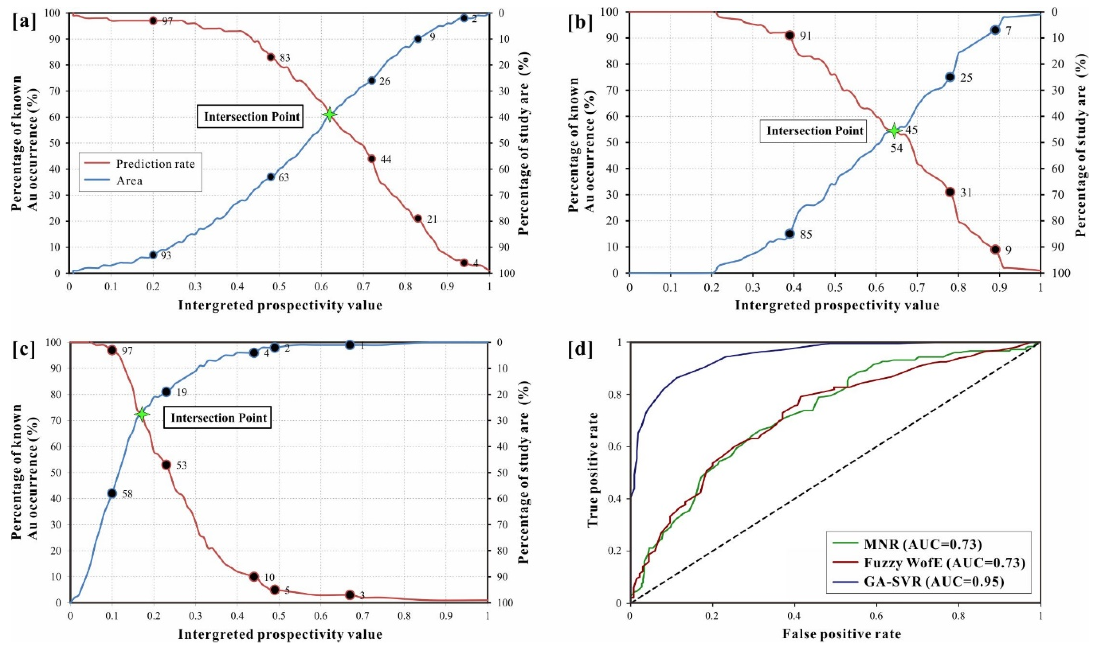
3.4.2. Comparison and Assessment

Known mineralization samples in the prospectivity space are thought to be an effective verification for model validity assessment [19,20,59]. To test the performance of SVR, another two typical methods, MNR and fuzzy WofE [69,70], a statistics evaluation model and a Bayesian probabilistic model were chosen as comparison methods.

The aforementioned methods were compared in terms of PA plot and ROC curve. In the P-A plot, two curves, namely the prediction-rate curve and the occupied area curve, are mapped for estimating the ability of each to predict mineralization, mineral occurrences and the sizes of predicted target areas [58]. Additionally, the point where curves intersect straightway reflects the probability of mineral deposit occurrence. When the intersection point shows a higher prediction rate and smaller occupied area, it indicates high mineralization probability. ROC curve, a validation technique widely used in machine learning, has been introduced into prospectivity models assessment [24,59,71]. It takes both the true positive rate and false positive rate into consideration. Additionally, the area under the ROC curve (AUC), with values varying from 0 to 1, can be used to measure the performance of prospectivity models. An AUC value of 1 indicates the result has perfect accuracy, whereas an AUC value below 0.5 determines the result is a random model [59,71].

4. Results

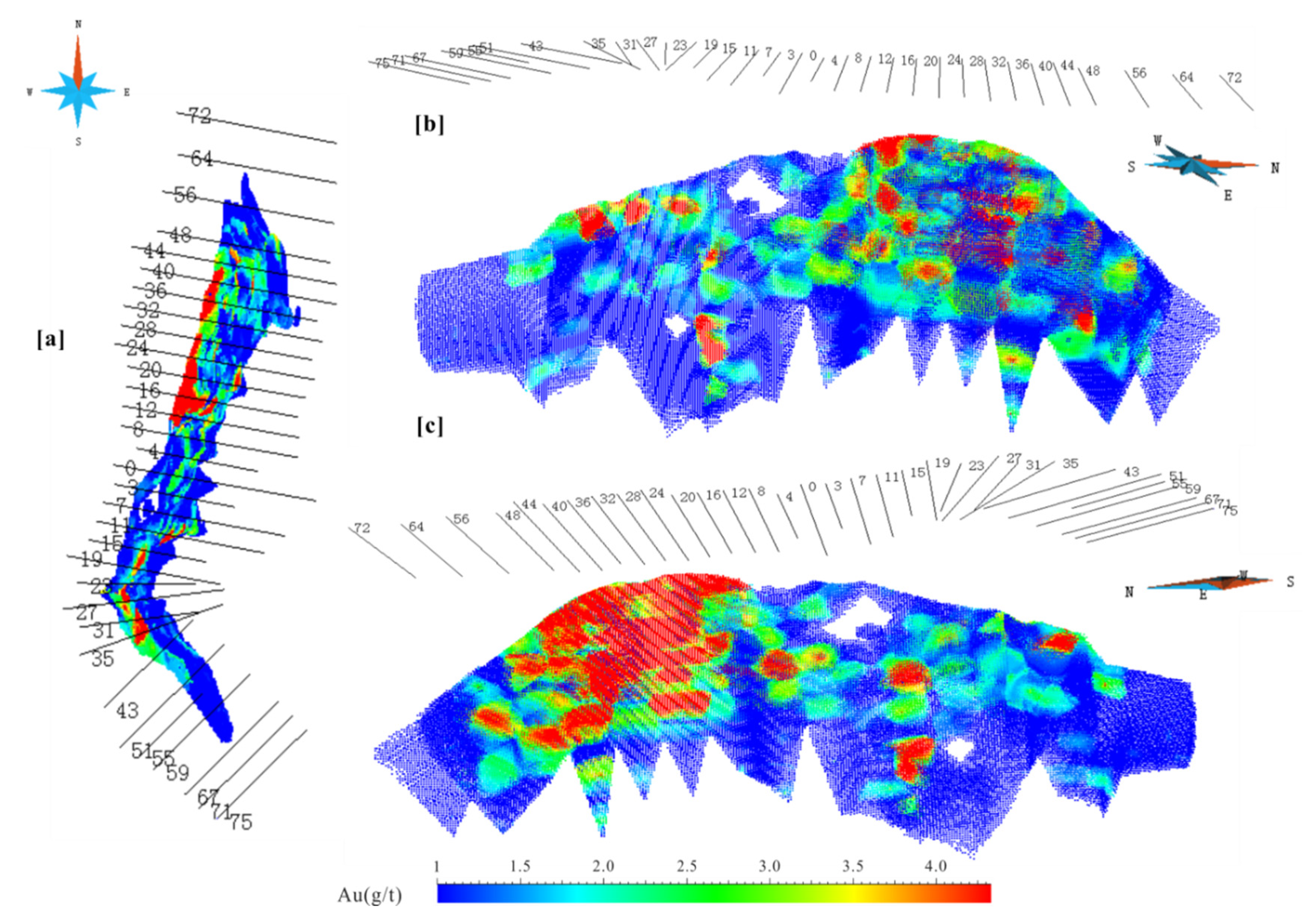
4.1. Gold Distribution

Based on the gold assay data and the 3D model of orebodies, gold grade (Au) was assigned to every voxel of orebodies via the 3D Kriging interpolation method [20,72]. The 3D assay model displays a discontinuous gold spatial distribution and an obvious gold-enrichment in the footwall of the orebody in the north domain (Figure 5). Gold mineralization with Au > 3 g/t in the north domain is mainly confined into sections of No. 48 and No. 12, where mineralization extends about 300 m from south to north. This area is a gently undulating (overall trend NNE) with a maximum thickness of orebody (about 40 m). In the northernmost orebody changes to NNW-striking, roughly paralleling with F₂ (Figure 2) and maintains a relatively high grade proximal to the fault. Industrial-grade mineralization occurs in the domain between sections No. 35 and No. 15 (Figure 5). This area is characterized by an arcuate zone, and high-grade mineralization occurs as a lens. Overall, the Axi orebodies expand in sections of No. 48–12 and No. 27–35 and bend in the vicinity of sections No. 44 and No. 23, emerging, enlarging and narrowing with undulations along the dip and strike (Figure 5).

4.2. Spatial Analysis of Geological Features

The spatial distance analysis results demonstrate that the higher values (yellow to red) of distance to F₂, LVP, and the upper interface of the phyllic alteration zone are similarly confined in the areas between sections No. 56 and No. 16, and No. 35 and No. 15. The dF, dGV and dAlt show overall lower values in the south and higher values in the north (Figure 6a–c). Gold occurrences are principally located in the hanging wall of F₂ and LVP lower interface with a distance of 0 to 50 m (Figure 6a,b), and in the footwall of phyllic alteration upper interface zone with a distance of 0 to −80 m (Figure 6c). Distinct bimodal distribution has been found between the gold grade and distances (dF, dGV, and dAlt) (Figure 7(a1–c1)), showing multiple-peak relationships with gold grade. For instance, the Au-dAlt has two peaks, the flat peak is in the range from 40 to 60 with a grade peak of 3.4 g/t, whereas the sharp peak centralizes closely to 95 with a grade peak of 3 g/t (Figure 7(c1)). However, the relationship between AuMet and distances (dF, dGV, and dAlt) is similar to left-skewed Gaussian distribution with peaks respectively in 30, 40 and 50 (Figure 7(a2–c2)).

The slope extraction results show that the highest values of gF are concentrated near-surface between sections No. 36 and No. 4, but at different depths between sections No. 11 and No. 27 (Figure 6d). The reverse is true for gAlt, which is lower at shallow depth (Figure 6f). Gold is concentrated in relatively sloped areas (>65°; Figure 7(d1–f1)). Analogously, there is a bimodal distribution between the slopes (gF, gGV, and gAlt) and grade (Figure 7(d1–f1)), such as Au vs. gF which has two peaks, 65° and 85° (Figure 7(d1)). A right-skewed distribution between the slope and AuMet demonstrates the segments with steeper slopes host a higher percentage of gold than other intervals (Figure 7(d2–f2)).

The morphological undulation analysis displays there are several distinct high-value centers of wrF, wrGV, and wrAlt in the areas between sections No. 48 to 32, No. 12 to 3, and No. 19 to 43, respectively (Figure 6g–i). Concentrated gold distribution areas of undulation (wrF, wrGV, and wrAlt) are in the interval of 0 to 20 m, −10 to 10 m, and 0 to 20 m, respectively (Figure 7(g1–i1)). The relationships between the undulation (wrF, wrGV, and wrAlt) and grade show a multimodal distribution (Figure 7(g1–i1)). Differing from the normal distribution of the other AuMet undulations, the relationship between AuMet and wrF is a bimodal distribution with two peaks of −2 and 16 (Figure 7(i2)).

4.3. The Efficiency of Prospectivity Models

The P-A plots of three prospectivity models show that GA-SVR had a prediction rate of 74% in 26% of the study area; 62% of the known ore voxels were predicted in 38% of the study area by MNR, and only 55% of the known occurrences were forecasted in 45% of the study area via fuzzy WofE (Figure 8a–c). In ROC curves, GA-SVR models with the AUC value of 0.95 exhibits a better performance of prospectivity, whereas MNR and fuzzy WofE are less accurate, with the same AUC value of 0.73 (Figure 8d).

4.4. Target Appraisal

Based on the criterion of the highest predictive score in the smallest occupied area, three exploration targets (targets I to III) with high-value mineralization probability have been inferred in the study area using the GA-SVR prospectivity model (Figure 9). Target I is located at a depth beneath the known orebody in the north segment and in the hanging wall of the fault F₂, with the burial depth of 440 m to 750 m. Close to the largest and economically productive orebody group, target I is most likely a group of deep, ore-forming fluid conduits stretching from the deep magmatic intrusion of the Axi deposit (see below discussion) and is considered as the highest priority target in the study area. Target II in the south part of the deposit occurs below the known orebodies and in the hanging wall of the fault F₂ as well, at a depth of >800 m. It is situated in the transitional zone of the fault, orebodies, and alteration zone. Target III is located to north stretching farther along the N-trend of known orebodies, with a depth of >1000 m, probably demonstrating that it is the north branch of the proven orebody.

5. Discussion

5.1. Insights from 3D Models and Spatial Analysis

Our spatial analysis shows that there is a bimodal distribution of gold grade (Au) and a single peak of gold resource (AuMet) in the pyrite-sericite-quartz alteration buffer field (Figure 7(c1)). Here, dAlt (40, 60) may represent the position of main orebodies, because of the higher grades (avg. up to 3.5 g/t) and approximate distance to width (about 20 m). The intervals of dAlt (0, 20) and dAlt (20, 40) most likely reflect the location of disseminated ore and the mixing zone of disseminated ore and quartz-sulfide stockwork, respectively, taking account of the value and increasing rate of Au and AuMet. Such vein-alteration distribution is well supported by field investigations (Figure 2). It is very interesting that almost all siliceous veins with gold mineralization are hosted in the phyllic alteration zone, with major vein-type orebodies located in their centers. Apparently, phyllic alteration, to some extent, controls the occurrence of late quartz veins that are products of distributed hydrothermal fluid infiltrating a brecciated zone [33]. However, the crosscutting relationship and 20 M.y. time gap between phyllic alteration and auriferous quartz veins preclude the coeval formation in one hydrothermal event [33,35,37,39]. Previous studies have proposed that the interactions between hydrothermal fluids and rocks could enhance the rock permeability by mass and volume changes linked to mineral dissolution and precipitation, and further control or facilitate the brecciation and formation of new fractures [73,74,75,76]. Since the fault F₂ underwent at least three-phases of deformation during strike-slip movement during ore-forming processes [41], the occurrence of quartz veins was mostly likely promoted by late structural deformation on the earlier altered rock.

Two major types of economic ore (i.e., disseminated and vein-type) at Axi are genetically related to early fluid-rock reactions during phyllic alteration and later fluid mixing and boiling in the fault damage zone [33,35,37,39]. The above mineralization mechanism is ubiquitous in LS epithermal gold deposits and is essentially attributed to fluid flow and convergence in the epithermal environment [2,3,6]. The 3D models and spatial analysis indicate that the morphological characteristics and distance field of geological features significantly control the distribution of gold resources in the Axi gold deposit. Specifically, the AuMet is commonly confined to the zones distance to F₂ (0–50 m), the LVP lower interface (10–60 m), and the phyllic upper interface (20–70 m), with high dipping angles of 65–75° and gentle undulation, but with increased frequency on convex areas (0–20 m; Figure 7). These characteristics underline the critical roles of these geological interfaces for driving and gathering ore-forming fluids at Axi. It is notable that all convex areas have high grade and resources (Figure 7(g1,g2)). This implies strain localization (or release) with orientation similar to global strain, accompanied gold deposition, and likely led to the brecciation or caused fluid preferential confluence in more outward bending areas at Axi.

The 3D models and distance field analysis reveal a rule that the alteration-mineralization zone in bending sites is clearly wider than the overall distribution (Figure 3), and notably, also have relatively high gold grades (Figure 7(c1)). Interestingly, these are locations where the main orebodies are comprised of quartz vein-type ores, suggesting at least a rough spatial or genetic correlation between vein-type orebodies and normal-strike slip extension deformation. The fragmentized contact zone ascribed to the overprinting structural deformation on the early altered zone may be the pathway and dilation space for hydrothermal fluid transmission [3,75,76]. In addition, the altered rocks near permeable channels commonly have different mechanical properties from nearby wall rocks, thereby showing distinct deformation during fault propagation, as discussed above. Thus, the quartz vein orebodies in the transition zone reflect the original location of fluid conduits, which is consistent with the empirical mineral assemblage of quartz/chalcedony-carbonates-adularia-sericite as the indicator for fluid conduits in the epithermal system [3,8,77,78]. We, therefore, infer that the major fluid conduits of the Axi epithermal gold deposit are located in the bending areas (No. 35–15 and No. 40–56).

5.2. Application of Support Vector Regression Model

The extracted metallogenic information in 3D prospectivity modeling of the Axi epithermal gold deposit has the following features: (1) non-linearity in that gold mineralization is spatially controlled by a series of geological factors with non-linear relationships [14,49,59]; (2) distribution diversification in that the ore-controlling indicators datasets exhibit different distribution statistics [23,24,25]; (3) high-dimensionality in that 9 predictor maps construct a nine-dimensional feature space [23,24,25].

In this study, the MNR method for integrating ore-forming information from the Axi epithermal gold deposit shows weak prospective ability. MNR has been proved fit for prospectivity modeling of deposits with a relatively mild grade and amount of metal variation, distributed normally [23,26]. However, the gold grade of Axi gold deposit changes sharply and yields a log-normal distribution (Figure 6), hence, MNR is a poor fit for prospectivity modeling of this LS epithermal gold deposit, and especially performs worse in fitting samples with erratic high-grade. Although the fuzzy WofE identified more known ore voxels in a smaller occupied space when compared to MNR, it did not produce a robust prospectivity model. In fuzzy WofE, spatially continuous predictor map values are first simplified and discretized into a series of arbitrary classes, and the same weight is assigned to all values in each class. This process is excessively dependent on expert knowledge, resulting in some geological information loss or inconsistencies, which would generate systemic bias in the weighting of spatial evidential layers in the prospectivity model [20,79]. Furthermore, multiple layer integration based on fuzzy WofE is analogous to a nonlinear multiplicative cascade process. Thus, the accuracy and reliability of predictive results may decline, if there is dependence or weak conditional independence between diverse predictive maps [57].

Both the PA plot and ROC curve indicated GA-SVR was superior to MNR and fuzzy WofE in delimiting exploration targets in the Axi gold deposit. These results could be interpreted in several ways:

(1)

As previously mentioned, the known Au-grade in Axi gold deposit changes sharply and unevenly distributes in space, resulting in the poor performance of traditional prospectivity methods (e.g., MNR and fuzzy WofE). Nevertheless, GA-SVR is able to overcome the aforesaid disadvantages, because of it is irrespective of data distribution and outliers, making better generalization performance [30,32,65,66].

(2)

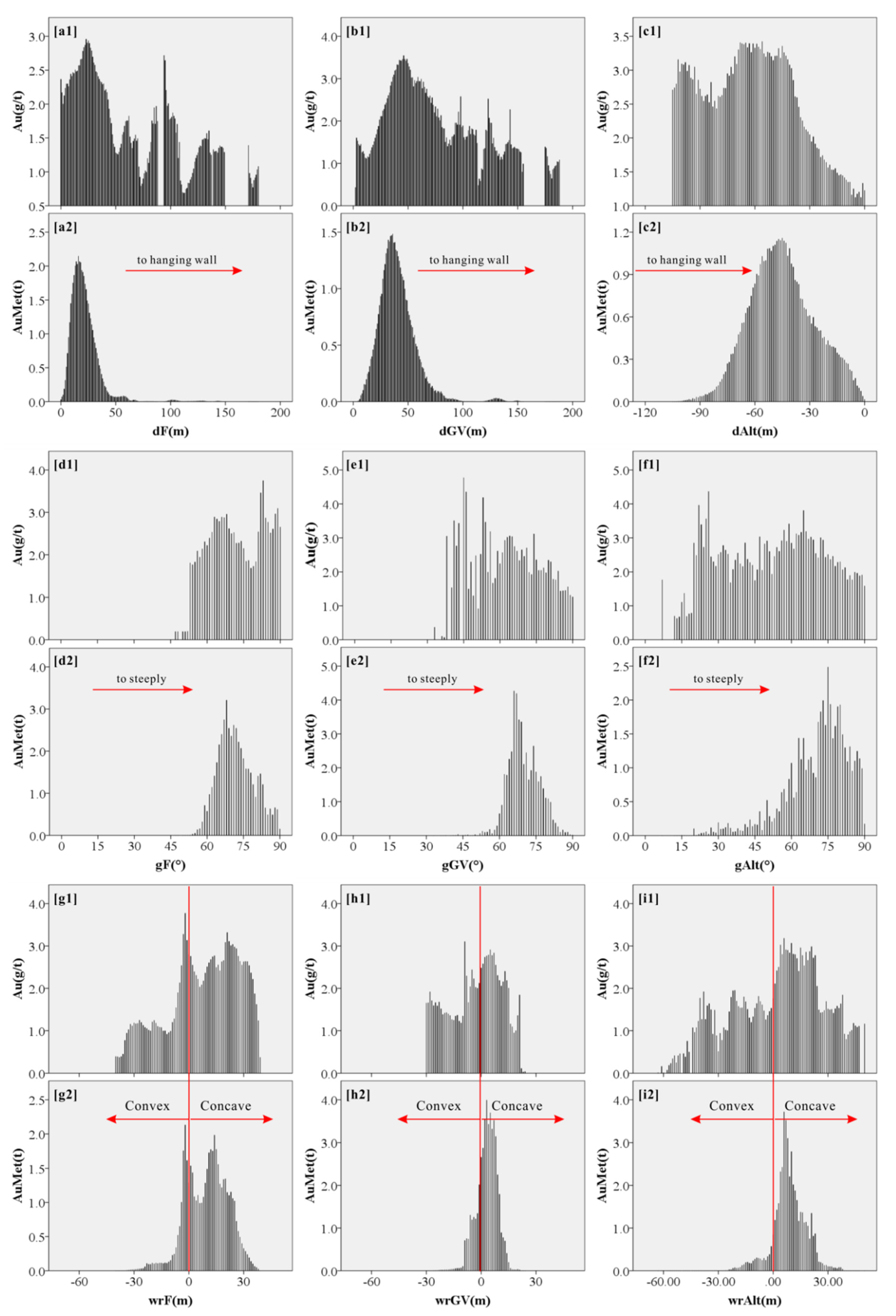
The spatial analysis results indicate that there is a complicated non-linear spatial association between gold occurrence and geological features, due to the superimposition of various geological events in the ore-forming processes that are difficult to quantify [57]. SVR, characterized by non-linearity, self-learning, and robustness, constructs a higher dimensional feature space from the lower dimensional input space via non-linear mapping [20,50,51]. Then, the complicated non-linear spatial association in the original low dimensional input space is treated as an oversimplified linear regression solution in high dimensional feature space, and therefore it can be commendably quantified and the prediction ability is improved [54,62].

(3)

There are many parameters that have to be determined using expert opinion in traditional prospectivity models (e.g., weight definition in fuzzy WofE), resulting in systemic bias and error [20,79]. By contrast, GA-SVR obtains optimal parameters that could produce the best prediction via GA with less subjectivity [30,32,61].

Consequently, the hybrid model of GA-SVR based on the combination of SVR and GA takes advantage both of GA and SVR in the prospecting modeling of the Axi gold deposit, and therefore is a promising method in 3D mineral prospectivity modeling.

5.3. Exploration Significanture for LS Epithermal Deposit

LS epithermal mineralization is typically developed at shallow depths in terms of the high-permeability networks favoring magmatic water ascent, external fluid influx, and the interplay of fluid and rock, thereby resulting in the extensional vein systems and intensive water-rock interactions [1,2,3,4,5,6,7]. These characteristics are clear in our 3D models and spatial analysis results and allow understanding of the metallogenic implications in the Axi LS epithermal gold deposit. In addition, the integration of obtained spatial data about F₂, LVP and the phyllic alteration zone controls on mineralization was used to identify the fertility of unknown areas at Axi. One of the targets in the northern Axi district is buried in the Aqialehe sedimentary formation and indicates ore-forming fluid migration along F₂ from conduits to the north in the shallow areas. This suggests a major horizontal fluid pathway controlled by structures in the epizonal segments of this LS epithermal deposit. Thus, in the exploration of epithermal mineralization in a mine, more attention should be given to the (sub-) horizontal extending directions from present orebodies with particular concern paid to the local structural deformation.

Although deep segments of ore fluid conduits host less gold in epithermal deposits, the areas could offer clues to find a new type of mineralization, such as base metal mineralization and porphyry [80,81]. Hence, determining as much as possible about the LS epithermal deposit fluid conduits, even at depth, has the potential to be quite valuable in guiding further mineral exploration. In this study, a comprehensive analysis of geological models and spatial analysis obtained important information about the ore fluid conduits in the Axi epithermal system that include the relative specific spatial location, meaningful geological indicators, and overprinting structural influences on up-flow zones. The above findings highlight the great potential of 3D geological modeling and spatial analysis in understanding the overprinting structural-hydrothermal processes and determining the location of fluid conduits.

In summary, the framework of 3D prospectivity modeling presented here, including 3D geological modeling, spatial analysis, and prospectivity modeling, can improve the understanding of ore genesis and allow for the improvement of exploration strategies in LS epithermal deposits. We encourage all LS mine operators and prospectors to develop similar models.

6. Conclusions

(1) The 3D prospectivity modeling for the Axi gold deposit quantitatively determines the spatial association between orebodies and geological features, and further improves evaluation of the mineralization potential in 3D space at the deposit-scale, and can aid in developing and enhancing mineral exploration strategies for the LS epithermal gold deposit.

(2) The hybrid model GA-SVR is proven to be better at quantifying the complicated non-linear spatial association between gold occurrence and geological features, with less subjectivity when compared to MNR and fuzzy WofE, demonstrating a better prediction capability in prospectivity mapping.

(3) The majority of gold mineralization in the Axi deposit is confined to zones close to fault F₂ (0–50 m), the LVP lower interface (10–60 m), and the phyllic alteration upper interface (20–70 m), with steeply dipping angles (>65°) and gentle undulation with priority on the convex areas (0–20 m). Two fluid conduits of the Axi epithermal gold deposit are speculated in sections No. 35–15 and No. 40–56.

(4) In future work, incorporating various geoscience data into 3D mineral prospectivity modeling, such as geochemical data, geophysical data, and remote sensing data, may be an effective step to provide more reliable exploration decision-making [82,83,84]. The deep learning (e.g., neuroevolution) with enormous potential in learning complicated functions is encouraged to be further applied for improving prospectivity modeling.

References

1. Hedenquist, J.W.; Arribas, A.; Gonzales-Urien, E. Exploration for epithermal gold deposits. Rev. Econ. Geol. 2000, 13, 245–277. [Google Scholar]
2. Sillitoe, R.H.; Hedenquist, J.W. Linkages between volcanotectonic settings, ore-fluid compositions, and epithermal precious metal deposits. In Volcanic, Geothermal, and Ore-Forming Fluids: Rulers and Witnesses of Processes within the Earth; Simmons, S.F., Graham, I., Eds.; Society of Economic Geologists, Inc.: Littleton, CO, USA, 2003; pp. 315–345. [Google Scholar]
3. Simmons, S.F.; White, N.C.; John, D.A. Geological characteristics of epithermal precious and base metal deposits. In Economic Geology One Hundredth Anniversary Volume 1905–2005 Society of Economic Geologists; Hedenquist, J.W., Thompson, J.F.H., Goldfarb, R.J., Richards, J.P., Eds.; Society of Economic Geologists, Inc.: Littleton, CO, USA, 2005; pp. 485–522. [Google Scholar]
4. Sillitoe, R.H. Epithermal paleosurfaces. Miner. Depos. 2015, 50, 767–793. [Google Scholar] [CrossRef]
5. Cooke, D.R.; Simmons, S.F. Characteristics and genesis of epithermal gold deposits. Rev. Econ. Geol. 2000, 13, 221–244. [Google Scholar]
6. John, D.A.; Hofstra, A.H.; Fleck, R.J.; Brummer, J.E.; Saderholm, E.C. Geologic setting and genesis of the Mule Canyon low-sulfidation epithermal gold-silver deposit, north-central Nevada. Econ. Geol. 2003, 98, 425–463. [Google Scholar] [CrossRef]
7. Clark, L.V.; Gemmell, J.B. Vein stratigraphy, mineralogy, and metal zonation of the kencana low-sulfidation epithermal Au–Ag deposit, Gosowong goldfield, Halmahera island, Indonesia. Econ. Geol. 2018, 113, 209–236. [Google Scholar] [CrossRef]
8. Simmons, S.F.; Browne, P.R. Hydrothermal minerals and precious metals in the Broadlands-Ohaaki geothermal system: Implications for understanding low-sulfidation epithermal environments. Econ. Geol. 2000, 95, 971–999. [Google Scholar] [CrossRef] [Green Version]
9. Henley, R.W. The geothermal framework of epithermal deposits. Rev. Econ. Geol. 1985, 2, 1–24. [Google Scholar]
10. Rowland, J.V.; Simmons, S.F. Hydrologic, magmatic, and tectonic controls on hydrothermal flow, Taupo Volcanic Zone, New Zealand: Implications for the formation of epithermal vein deposits. Econ. Geol. 2012, 107, 427–457. [Google Scholar] [CrossRef]
11. John, D.A.; Vikre, P.G.; du Bray, E.A.; Blakely, R.J.; Fey, D.L.; Rockwell, B.W.; Mauk, J.L.; Anderson, E.D.; Graybeal, F.T. Descriptive Models for Epithermal Gold-Silver Deposits: Chapter Q in MINERAL Deposit Models for Resource Assessment (No. 2010-5070-Q); US Geological Survey: Reston, VA, USA, 2018.
12. Cox, S.F.; Knackstedt, M.A.; Brown, J. Principle of structural control on permeability and fluid flow in hydrothermal systems. In Structural Control on Ore Genesis; Richards, J.P., Tosdal, R.M., Eds.; Society of Economic Geologists, Inc.: Littleton, CO, USA, 2001; Volume 14, pp. 1–24. [Google Scholar]
13. Berger, B.R.; Tingley, J.V.; Drew, L.J. Structural localization and origin of compartmentalized fluid flow, Comstock Lode, Virginia City, Nevada. Econ. Geol. 2003, 98, 387–408. [Google Scholar] [CrossRef]
14. Carranza, E.J.M. Controls on mineral deposit occurrence inferred from analysis of their spatial pattern and spatial association with geological features. Ore Geol. Rev. 2009, 35, 383–400. [Google Scholar] [CrossRef]
15. Xiao, F.; Chen, J.; Hou, W.; Wang, Z.; Zhou, Y.; Erten, O. A spatially weighted singularity mapping method applied to identify epithermal Ag and Pb-Zn polymetallic mineralization associated geochemical anomaly in Northwest Zhejiang, China. J. Geochem. Explor. 2018, 189, 122–137. [Google Scholar] [CrossRef]
16. De Palomera, P.A.; van Ruitenbeek, F.J.; Carranza, E.J.M. Prospectivity for epithermal gold–silver deposits in the Deseado Massif, Argentina. Ore Geol. Rev. 2015, 71, 484–501. [Google Scholar] [CrossRef]
17. Li, N.; Bagas, L.; Li, X.H.; Xiao, K.Y.; Li, Y.; Ying, L.J.; Song, X.L. An improved buffer analysis technique for model-based 3D mineral potential mapping and its application. Ore Geol. Rev. 2016, 76, 94–107. [Google Scholar] [CrossRef]
18. Mao, X.; Zhang, B.; Deng, H.; Zou, Y.; Chen, J. Three-dimensional morphological analysis method for geologic bodies and its parallel implementation. Comput. Geosci. 2016, 96, 11–22. [Google Scholar] [CrossRef]
19. Zhang, M.; Zhou, G.; Shen, L.; Zhao, W.; Liao, B.; Yuan, F.; Li, X.; Hu, X.; Wang, C. Comparison of 3D prospectivity modeling methods for Fe–Cu skarn deposits: A case study of the Zhuchong Fe–Cu deposit in the Yueshan orefield (Anhui), eastern China. Ore Geol. Rev. 2019, 114, 103126. [Google Scholar] [CrossRef]
20. Mao, X.; Ren, J.; Liu, Z.; Chen, J.; Tang, L.; Deng, H.; Bayless, R.C.; Yang, B.; Wang, M.; Liu, C. Three-dimensional prospectivity modeling of the Jiaojia-type gold deposit, Jiaodong Peninsula, Eastern China: A case study of the Dayingezhuang deposit. J. Geochem. Explor. 2019, 203, 27–44. [Google Scholar] [CrossRef]
21. Qin, Y.Z.; Liu, L.M. Quantitative 3D Association of Geological Factors and Geophysical Fields with Mineralization and Its Significance for Ore Prediction: An Example from Anqing Orefield, China. Minerals 2018, 8, 300. [Google Scholar] [CrossRef] [Green Version]
22. Yuan, F.; Li, X.H.; Zhang, M.M.; Jowitt, S.M.; Jia, C.; Zheng, T.K.; Zhou, T.F. Three-dimensional weights of evidence-based prospectivity modeling: A case study of the Baixiangshan mining area, Ningwu Basin, Middle and Lower Yangtze Metallogenic Belt, China. J. Geochem. Explor. 2014, 145, 82–97. [Google Scholar] [CrossRef]
23. Carranza, E.J.M.; Laborte, A.G. Data-driven predictive mapping of gold prospectivity, Baguio district, Philippines: Application of Random Forests algorithm. Ore Geol. Rev. 2015, 71, 777–787. [Google Scholar] [CrossRef]
24. Rodriguez-Galiano, V.; Sanchez-Castillo, M.; Chica-Olmo, M.; Chica-Rivas, M. Machine learning predictive models for mineral prospectivity: An evaluation of neural networks, random forest, regression trees and support vector machines. Ore Geol. Rev. 2015, 71, 804–818. [Google Scholar] [CrossRef]
25. Sun, T.; Chen, F.; Zhong, L.; Liu, W.; Wang, Y. GIS-based mineral prospectivity mapping using machine learning methods: A case study from Tongling ore district, eastern China. Ore Geol. Rev. 2019, 109, 26–49. [Google Scholar] [CrossRef]
26. Porwal, A.; Carranza, E.J.M.; Hale, M. Artificial Neural Networks for Mineral-Potential Mapping: A Case Study from Aravalli Province, Western India. Nat. Resour. Res. 2003, 12, 155–171. [Google Scholar] [CrossRef]
27. Harris, J.R.; Grunsky, E.; Behnia, P.; Corrigan, D. Data- and knowledge-driven mineral prospectivity maps for Canada’s North. Ore Geol. Rev. 2015, 71, 788–803. [Google Scholar] [CrossRef]
28. Juliani, C.; Ellefmo, S.L. Prospectivity Mapping of Mineral Deposits in Northern Norway Using Radial Basis Function Neural Networks. Minerals 2019, 9, 131. [Google Scholar] [CrossRef] [Green Version]
29. Hong, W.C.; Dong, Y.; Zhang, W.Y.; Chen, L.Y.; Panigrahi, B.K. Cyclic electric load forecasting by seasonal SVR with chaotic genetic algorithm. Int. J. Electr. Power 2013, 44, 604–614. [Google Scholar] [CrossRef]
30. Oyehan, T.A.; Alade, I.O.; Bagudu, A.; Sulaiman, K.O.; Olatunji, S.O.; Saleh, T.A. Predicting of the refractive index of haemoglobin using the Hybrid GA-SVR approach. Comput. Biol. Med. 2018, 98, 85–92. [Google Scholar] [CrossRef]
31. Tang, X.; Wang, L.; Cheng, J.; Chen, J.; Sheng, V. Forecasting Model Based on Information-Granulated GA-SVR and ARIMA for Producer Price Index. Tech Sci. Press 2019, 58, 463–491. [Google Scholar] [CrossRef] [Green Version]
32. Roushangar, K.; Koosheh, A. Evaluation of GA-SVR method for modeling bed load transport in gravel-bed rivers. J. Hydrol. 2015, 527, 1142–1152. [Google Scholar] [CrossRef]
33. An, F.; Zhu, Y. Geology and geochemistry of the Early Permian Axi low-sulfidation epithermal gold deposit in North Tianshan (NW China). Ore Geol. Rev. 2018, 100, 12–30. [Google Scholar] [CrossRef]
34. Zhang, B.; Li, N.; Shu, S.P.; Wang, W.; Yu, J.; Chen, X.; Ye, T.; Chen, Y.J. Textural and compositional evolution of Au-hosting Fe–S–As minerals at the Axi epithermal gold deposit, Western Tianshan, NW China. Ore Geol. Rev. 2018, 100, 31–50. [Google Scholar] [CrossRef]
35. Liu, Z.; Mao, X.; Deng, H.; Li, B.; Zhang, S.; Lai, J.; Bayless, R.C.; Pan, M.; Li, L.; Shang, Q. Hydrothermal processes at the Axi epithermal Au deposit, western Tianshan: Insights from geochemical effects of alteration, mineralization and trace elements in pyrite. Ore Geol. Rev. 2018, 102, 368–385. [Google Scholar] [CrossRef]
36. Zhai, W.; Sun, X.; Sun, W.; Su, L.; He, X.; Wu, Y. Geology, geochemistry, and genesis of Axi: A Paleozoic low-sulfidation type epithermal gold deposit in Xinjiang, China. Ore Geol. Rev. 2009, 36, 265–281. [Google Scholar] [CrossRef]
37. Liu, Z.; Mao, X.; Ackerman, L.; Li, B.; Dick, J.M.; Yu, M.; Peng, J.; Shahzad, S.M. Two-stage gold mineralization of the Axi epithermal Au deposit, Western Tianshan, NW China: Evidence from Re–Os dating, S isotope, and trace elements of pyrite. Miner. Depos. 2019. [Google Scholar] [CrossRef]
38. Zhao, X.; Xue, C.; Chi, G.; Wang, H.; Qi, T. Epithermal Au and polymetallic mineralization in the Tulasu Basin, western Tianshan, NW China: Potential for the discovery of porphyry CuAu deposits. Ore Geol. Rev. 2014, 60, 76–96. [Google Scholar] [CrossRef]
39. An, F.; Zhu, Y.; Wei, S.; Lai, S. An Early Devonian to Early Carboniferous volcanic arc in North Tianshan, NW China: Geochronological and geochemical evidence from volcanic rocks. J. Asian Earth Sci. 2013, 78, 100–113. [Google Scholar] [CrossRef]
40. Tang, G.J.; Wang, Q.; Wyman, D.A.; Sun, M.; Zhao, Z.H.; Jiang, Z.Q. Petrogenesis of gold-mineralized magmatic rocks of the Taerbieke area, northwestern Tianshan (western China), Constraints from geochronology, geochemistry and Sr–Nd–Pb–Hf isotopic compositions. J. Asian Earth Sci. 2013, 74, 113–128. [Google Scholar] [CrossRef]
41. Wei, J.L.; Cao, X.Z.; Xu, B.J.; Zhang, W.S.; Rao, D.P.; Huang, L.W. Erosion and post-mineralization change of Axi epithermal gold deposit in Western Tianshan Mountains. Miner. Depos. 2014, 33, 241–254. (In Chinese) [Google Scholar]
42. Jessell, M.; Ailleres, L.; De Kemp, E.; Lindsay, M.; Wellmann, F.; Hillier, M.; Laurent, G.; Carmichael, T.; Martin, R. Next Generation Three-Dimensional Geologic Modeling and Inversion. In Building Exploration Capability for the 21st Century; Kelley, K.D., Golden, H.C., Eds.; Soc Economic Geologists, Inc.: Littleton, CO, USA, 2014; pp. 261–272. [Google Scholar]
43. Li, X.; Yuan, F.; Zhang, M.; Jowitt, S.M.; Ord, A.; Zhou, T.; Dai, W. 3D computational simulation-based mineral prospectivity modeling for exploration for concealed Fe–Cu skarn-type mineralization within the Yueshan orefield, Anqing district, Anhui Province, China. Ore Geol. Rev. 2019, 105, 1–17. [Google Scholar] [CrossRef]
44. Li, N.; Song, X.; Xiao, K.; Li, S.; Li, C.; Wang, K. Part II: A demonstration of integrating multiple-scale 3D modelling into GIS-based prospectivity analysis: A case study of the Huayuan-Malichang district, China. Ore Geol. Rev. 2018, 95, 292–305. [Google Scholar] [CrossRef]
45. Sporli, K.B.; Cargill, H. Structural Evolution of a World-Class Epithermal Orebody: The Martha Hill Deposit, Waihi, New Zealand. Econ. Geol. 2011, 106, 975–998. [Google Scholar] [CrossRef] [Green Version]
46. Jowitt, S.M.; Cooper, K.; Squire, R.J.; Thebaud, N.; Fisher, L.A.; Cas, R.A.F.; Pegg, I. Geology, mineralogy, and geochemistry of magnetite-associated Au mineralization of the ultramafic-basalt greenstone hosted Crusader Complex, Agnew Gold Camp, Eastern Yilgarn Craton, Western Australia; a Late Archean intrusion-related Au deposit? Ore Geol. Rev. 2014, 56, 53–72. [Google Scholar] [CrossRef]
47. Mao, X.; Tang, Y.; Lai, J.; Zou, Y.; Chen, J.; Peng, S.; Shao, Y.J. Three Dimensional Structure of Metallogenic Geologic Bodies in the Fenghuangshan Ore Field and Ore-controlling Geological Factors. Acta Geol. Sin. 2011, 85, 1507–1518. (In Chinese) [Google Scholar]
48. Mao, X.; Zhao, Y.; Tang, Y.; Peng, Z.; Chen, J.; Deng, H. Three-dimensional morphological analysis method for geological interfaces based on TIN and its application. J. Cent. South Univ. 2013, 44, 1493–1499. (In Chinese) [Google Scholar]
49. Zuo, R. A nonlinear controlling function of geological features on magmatic-hydrothermal mineralization. Sci. Rep. 2016, 6, 27127. [Google Scholar] [CrossRef] [PubMed]
50. Abedi, M.; Norouzi, G.-H.; Bahroudi, A. Support vector machine for multi-classification of mineral prospectivity areas. Comput. Geosci. 2012, 46, 272–283. [Google Scholar] [CrossRef]
51. Zuo, R.; Carranza, E.J.M. Support vector machine: A tool for mapping mineral prospectivity. Comput. Geosci. 2011, 37, 1967–1975. [Google Scholar] [CrossRef]
52. Shabankareh, M.; Hezarkhani, A. Application of support vector machines for copper potential mapping in Kerman region, Iran. J. Afr. Earth Sci. 2017, 128, 116–126. [Google Scholar] [CrossRef]
53. Carranza, E.J.M. Geocomputation of mineral exploration targets. Comput. Geosci. 2011, 37, 1907–1916. [Google Scholar] [CrossRef]
54. Li, X.; Luo, A.; Li, J.; Li, Y. Air Pollutant Concentration Forecast Based on Support Vector Regression and Quantum-Behaved Particle Swarm Optimization. Environ. Model. Assess. 2018, 24, 205–222. [Google Scholar] [CrossRef]
55. Santamaria-Bonfil, G.; Reyes-Ballesteros, A.; Gershenson, C. Wind speed forecasting for wind farms: A method based on support vector regression. Renew. Energy 2016, 85, 790–809. [Google Scholar] [CrossRef]
56. Patel, A.K.; Chatterjee, S.; Gorai, A.K. Development of a machine vision system using the support vector machine regression (SVR) algorithm for the online prediction of iron ore grades. Earth Sci. Inf. 2019, 12, 197–210. [Google Scholar] [CrossRef]
57. Cheng, Q. Non-Linear Theory and Power-Law Models for Information Integration and Mineral Resources Quantitative Assessments. Math. Geosci. 2008, 40, 503–532. [Google Scholar] [CrossRef]
58. Yousefi, M.; Carranza, E.J.M. Prediction–area (P–A) plot and C–A fractal analysis to classify and evaluate evidential maps for mineral prospectivity modeling. Comput. Geosci. 2015, 79, 69–81. [Google Scholar] [CrossRef]
59. Nykänen, V.; Lahti, I.; Niiranen, T.; Korhonen, K. Receiver operating characteristics (ROC) as validation tool for prospectivity models—A magmatic Ni–Cu case study from the Central Lapland Greenstone Belt, Northern Finland. Ore Geol. Rev. 2015, 71, 853–860. [Google Scholar] [CrossRef]
60. Vapnik, V.N. The Nature of Statistical Learning Theory; Springer: New York, NY, USA, 1995. [Google Scholar] [CrossRef] [Green Version]
61. Wang, L.; Wang, C.; Khoshnevisan, S.; Ge, Y.; Sun, Z. Determination of two-dimensional joint roughness coefficient using support vector regression and factor analysis. Eng. Geol. 2017, 231, 238–251. [Google Scholar] [CrossRef]
62. Wang, J.; Li, Y. Short-Term Wind Speed Prediction Using Signal Preprocessing Technique and Evolutionary Support Vector Regression. Neural Process. Lett. 2017, 48, 1043–1061. [Google Scholar] [CrossRef]
63. Scholkopf, B.; Sung, K.K.; Burges, C.J.C.; Girosi, F.; Niyogi, P.; Poggio, T. Comparing support vector machines with Gaussian kernels to radial basis function classifiers. IEEE Trans. Signal Proces. 1997, 45, 2758–2765. [Google Scholar] [CrossRef] [Green Version]
64. Ghaedi, M.; Dashtian, K.; Ghaedi, A.M.; Dehghanian, N. A hybrid model of support vector regression with genetic algorithm for forecasting adsorption of malachite green onto multi-walled carbon nanotubes: Central composite design optimization. Phys. Chem. Chem. Phys. 2016, 18, 13310–13321. [Google Scholar] [CrossRef]
65. Xin, N.; Gu, X.F.; Wu, H.; Hu, Y.Z.; Yang, Z.L. Application of genetic algorithm-support vector regression (GA-SVR) for quantitative analysis of herbal medicines. J. Chemom. 2012, 26, 353–360. [Google Scholar] [CrossRef]
66. Liu, S.; Tai, H.; Ding, Q.; Li, D.; Xu, L.; Wei, Y. A hybrid approach of support vector regression with genetic algorithm optimization for aquaculture water quality prediction. Math. Comput. Model. 2013, 58, 458–465. [Google Scholar] [CrossRef]
67. Stanley, K.O.; Clune, J.; Lehman, J.; Miikkulainen, R. Designing neural networks through neuroevolution. Nat. Mach. Intell. 2019, 1, 24–35. [Google Scholar] [CrossRef]
68. Chang, C.C.; Lin, C.J. LIBSVM: A Library for Support Vector Machines. ACM Trans. Intell. Syst. Technol. 2011, 2. [Google Scholar] [CrossRef]
69. Cheng, Q.M.; Agterberg, F.P. Fuzzy Weights of Evidence Method and Its Application in Mineral Potential Mapping. Nat. Resour. Res. 1999, 8, 27–35. [Google Scholar] [CrossRef]
70. Mao, X.; Zou, Y.; Lu, X.; Wu, X.; Dai, T. Quantitative analysis of geological ore-controlling factors and stereoscopic quantitative prediction of concealed ore bodies. J. Cent. South Univ. Technol. 2009, 16, 0987–0993. [Google Scholar] [CrossRef]
71. Bradley, A.P. The use of the area under the ROC curve in the evaluation of machine learning algorithms. Pattern Recogn. 1997, 30, 1145–1159. [Google Scholar] [CrossRef] [Green Version]
72. Xiao, K.Y.; Li, N.; Alok, P.; Holden, E.J.; Leon, B.; Lu, Y.J. GIS-based 3D prospectivity mapping: A case study of Jiama copper-polymetallic deposit in Tibet, China. Ore Geol. Rev. 2015, 71, 611–632. [Google Scholar] [CrossRef]
73. Sibson, R.H. Structural permeability of fluid-driven fault-fracture meshes. J. Struct. Geol. 1996, 18, 1031–1042. [Google Scholar] [CrossRef]
74. Micklethwaite, S. Mechanisms of faulting and permeability enhancement during epithermal mineralisation: Cracow goldfield, Australia. J. Struct. Geol. 2009, 31, 288–300. [Google Scholar] [CrossRef]
75. Williams, J.N.; Toy, V.G.; Smith, S.A.F.; Boulton, C. Fracturing, fluid-rock interaction and mineralisation during the seismic cycle along the Alpine Fault. J. Struct. Geol. 2017, 103, 151–166. [Google Scholar] [CrossRef]
76. Yang, L.; Zhao, R.; Wang, Q.F.; Liu, X.F.; Carranza, E.J.M. Fault geometry and fluid-rock reaction: Combined controls on mineralization in the Xinli gold deposit, Jiaodong Peninsula, China. J. Struct. Geol. 2018, 111, 14–26. [Google Scholar] [CrossRef]
77. De Palomera, P.A.; van Ruitenbeek, F.J.A.; van der Meer, F.D.; Fernandez, R. Geochemical indicators of gold-rich zones in the La Josefina epithermal deposit, Deseado Massif, Argentina. Ore Geol. Rev. 2012, 45, 61–80. [Google Scholar] [CrossRef]
78. Chang, Z.S.; Hedenquist, J.W.; White, N.C.; Cooke, D.R.; Roach, M.; Deyell, C.L.; Garcia, J.; Gemmell, J.B.; McKnight, S.; Cuison, A.L. Exploration Tools for Linked Porphyry and Epithermal Deposits: Example from the Mankayan Intrusion-Centered Cu–Au District, Luzon, Philippines. Econ. Geol. 2011, 106, 1365–1398. [Google Scholar] [CrossRef] [Green Version]
79. Yousefi, M.; Carranza, E.J.M. Fuzzification of continuous-value spatial evidence for mineral prospectivity mapping. Comput. Geosci. 2015, 74, 97–109. [Google Scholar] [CrossRef]
80. Spry, P.G.; Paredes, M.M.; Foster, F.; Truckle, J.S.; Chadwick, T.H. Evidence for a genetic link between gold-silver telluride and porphyry molybdenum mineralization at the Golden Sunlight Deposit, Whitehall, Montana; fluid inclusion and stable isotope studies. Econ. Geol. 1996, 91, 507–526. [Google Scholar] [CrossRef]
81. Sillitoe, R.H. Some metallogenic features of gold and copper deposits related to alkaline rocks and consequences for exploration. Miner. Depos. 2002, 37, 4–13. [Google Scholar] [CrossRef]
82. Farahbakhsh, E.; Chandra, R.; Eslamkish, T.; Müller, R.D. Modeling geochemical anomalies of stream sediment data through a weighted drainage catchment basin method for detecting porphyry Cu–Au mineralization. J. Geochem. Explor. 2019, 204, 12–32. [Google Scholar] [CrossRef]
83. Scalzo, R.; Kohn, D.; Olierook, H.; Houseman, G.; Chandra, R.; Girolami, M.; Cripps, S. Efficiency and robustness in Monte Carlo sampling for 3-D geophysical inversions with Obsidian v0.1.2: Setting up for success. Geosci. Model. Dev. 2019, 12, 2941–2960. [Google Scholar] [CrossRef] [Green Version]
84. Farahbakhsh, E.; Chandra, R.; Olierook, H.K.H.; Scalzo, R.; Clark, C.; Reddy, S.M.; Mueller, R.D. Computer vision-based framework for extracting tectonic lineaments from optical remote sensing data. Int. J. Remote Sens. 2020, 41, 1760–1787. [Google Scholar] [CrossRef]
Figure 1. (a) Geological map of the Tulasu basin showing the locations of porphyry and epithermal deposits. (b) Geological map of the Axi district. Both subfigures are based on Liu et al. [35].
Minerals 10 00233 g001
Figure 2. Representative cross-section (Line 48 on Figure 1b) illustrating the spatial relationships among orebodies, alteration, and fault in the Axi deposit. After Liu et al. [37].
Minerals 10 00233 g002
Figure 3. Above; 3D geological models of orebodies, phyllic alteration zone, late volcanic phase (LVP), and fault F2 in the Axi gold deposit.
Minerals 10 00233 g003
Figure 4. Genetic algorithm optimized support vector regression (GA-SVR) flowchart involved in prospectivity modeling for the Axi epithermal gold deposit.
Minerals 10 00233 g004
Figure 5. Above; 3D assay models showing the spatial distribution of gold grade of each voxel in the horizontal (a) and vertical (b,c) directions in the Axi deposit.
Minerals 10 00233 g005
Figure 6. Above; 3D raster models showing the distribution of geological features of the Axi deposit. (a) dF (distance value to F2); (b) dGV (distance value to the lower interface of LVP); (c) dAlt (distance value to the upper interface of the phyllic alteration zone); (d) gF (slope of F2); (e) gGV (slope of the lower interface of LVP); (f) gAlt (slope of the upper interface of the phyllic alteration zone); (g) wrF (undulation of F2); (h) wrGV (undulation of the lower interface of LVP); and (i) wrAlt (undulation of the upper interface of the phyllic alteration zone).
Minerals 10 00233 g006
Figure 7. Bar charts of geological features and mineralization indexes. (a) dF v.s. Au and AuMet; (b) dGV v.s. Au and AuMet; (c) dAlt v.s. Au and AuMet; (d) gF v.s. Au and AuMet; (e) gGV v.s. Au and AuMet; (f) gAlt v.s. Au and AuMet; (g) wrF v.s. Au and AuMet; (h) wrGV v.s. Au and AuMet; (i) wrAlt v.s. Au and AuMet. Au stands for the gold grade, and AuMet is the gold resource summation of all ore voxels in the same factor value.
Minerals 10 00233 g007
Figure 8. Prediction-area (P-A) plots and receiver operating characteristic (ROC) curves for different prospectivity models. (a) PA plot of MNR; (b) PA plot of fuzzy weights-of-evidence (WofE); (c) PA plot of GA-SVR; (d) ROC curves of three prospectivity models.
Minerals 10 00233 g008
Figure 9. Targets determined by the 3D prospectivity modeling of the Axi gold deposit.
Minerals 10 00233 g009