Abstract
The understanding of the dissolution and precipitation of minerals and its impact on the transport of fluids in porous media is essential for various subsurface applications, including shale gas production using hydraulic fracturing (“fracking”), CO2 sequestration, or geothermal energy extraction. In this work, we conducted a flow through column experiment to investigate the effect of barite precipitation following the dissolution of celestine and consequential permeability changes. These processes were assessed by a combination of 3D non-invasive magnetic resonance imaging, scanning electron microscopy, and conventional permeability measurements. The formation of barite overgrowths on the surface of celestine manifested in a reduced transverse relaxation time due to its higher magnetic susceptibility compared to the original celestine. Two empirical nuclear magnetic resonance (NMR) porosity–permeability relations could successfully predict the observed changes in permeability by the change in the transverse relaxation times and porosity. Based on the observation that the advancement of the reaction front follows the square root of time, and micro-continuum reactive transport modelling of the solid/fluid interface, it can be inferred that the mineral overgrowth is porous and allows the diffusion of solutes, thus affecting the mineral reactivity in the system. Our current investigation indicates that the porosity of the newly formed precipitate and consequently its diffusion properties depend on the supersaturation in solution that prevails during precipitation.
1. Introduction
Mineral precipitation and consequential changes in transport properties of porous media is of major interest for various natural and man-made systems ([1,2] and references therein). In particular, barite (BaSO4) is known to precipitate during oil and gas extraction, reducing the permeability of reservoir rocks and consequently decrease the extraction efficiency [3,4]. Moreover, in geothermal reservoirs and hydraulic fracturing of shales, barite precipitation is likely to occur in fractured zones [5,6,7]. Regarding nuclear waste disposal, barite can be an important secondary phase with respect to the retention of radium by the formation of (BaSO4-RaSO4) solid solutions [8,9,10]. As a result, barite precipitation mechanisms in porous media have been widely studied (e.g., [11,12,13,14,15]). However, so far only few studies provided quantitative assessment of barite precipitation in porous media and the consequential evolution of solute transport properties (e.g., permeability and diffusivity).
In a recent study, Poonoosamy et al. conducted a series of flow through column experiments to investigate the effect of supersaturation on barite precipitation mechanisms in porous media and consequential permeability changes [16]. These experiments served as an experimental benchmark for the validation of the implementation of conceptual models in reactive transport codes. The authors found that the Kozeny-Carman equation distinctively underestimated the permeability changes observed in the experiments, although it is widely applied in many reactive transport codes in a simplified form for describing porosity and permeability changes due to mineral dissolution and precipitation [1,2,17]. The Kozeny-Carman equation predicts fairly well the hydraulic conductivity of most soils with some exceptions involving heterogeneity or unconnected porosities (e.g., [18,19]). This is because the empirical relationship does not account for the changes in the microstructure and the pore architecture of the porous medium, such as pore throat distributions and connectivity of the pore network [20,21]. In fact, the Kozeny-Carman equation was not originally developed to describe the permeability changes of porous media undergoing alteration in its pore architecture [22].
Capturing local processes is important for the interpretation of permeability changes observed at macro-scale and requires the application of non-invasive imaging methods. Amongst these, nuclear magnetic resonance (NMR) including relaxometry (nuclear magnetic resonance relaxometry, NMRR) and imaging (magnetic resonance imaging, MRI) are valuable tools for the investigation of liquids and precipitation processes in porous media [23,24,25,26,27].
In this work, we investigate the use of a combination of NMRR and MRI for a better understanding of the effects of barite precipitation on the changes in porosity and permeability in porous medium. Although NMRR is a widely used technique to determine rock properties such as porosity and pore connectivity, its application to monitor the evolution of dissolution and precipitation processes in porous media is to our knowledge not well explored [27]. In addition, we test the conventional NMR porosity-permeability relationships, which are used to calculate the permeability from relaxometry measurements and verify their applicability for evolving porous media due to mineral dissolution/precipitation [28]. The experimental model system used in our study follow Poonoosamy et al., selecting the boundary conditions that led to different barite growth mechanisms in a single experiment [16].
2. Theory of MRI
MRI is based on the NMR effect which is, besides chemical analysis and biomedical imaging, widely used to study the water dynamics in porous media. Its principle relies on the nuclear magnetism linked with the spin of certain atomic nuclei. In case of water these are the hydrogen nuclei with spin = ½. When placed in an external magnetic field, two discrete energy states exist (Zeeman splitting). In an ensemble of spins the lower energy state is slightly higher populated according to Boltzmann’s statistical distribution, and ensemble averaging leads to macroscopic magnetization pointing along the direction of the external magnetic field (z-direction). The spin system can be excited by irradiation with electromagnetic waves, e.g., by a radio-frequency (rf) pulse in pulsed NMR, under the resonance condition that the energy gap between both states is proportional to the irradiation frequency (Larmor frequency) so that the macroscopic magnetization now precesses in the xy-plane perpendicular to the z-axis. This precessing transverse magnetization creates an electric current induced in a coil around the sample and is measured in NMR experiments. Subsequently, the system relaxes back to equilibrium with two different decay processes: transverse relaxation (T2) due to dephasing of individual spins and restoration of the thermal equilibrium by longitudinal relaxation (T1). Both relaxation processes control the measurable signal S(t) in ideal cases after a 90° exciting rf-pulse:
where S0 is proportional to the so-called spin density, i.e., water or liquid content, in the system under investigation, and tR is the repletion time between successive rf-excitations. The wealth of NMR methods is found in the multiple ways to manipulate the signal by combinations of additional rf-pulses and pulses of magnetic field gradient. The entire, time dependent set of the different pulses is termed as pulse sequence and is controlled by several pulse sequence parameters. An important one is the so-called spin-echo sequence, where the dephased, precessing magnetization in the xy-plane is rephased by a second rf-pulse, which creates a spin-echo. It’s intensity is controlled by the experimental parameters echo time, tE, repetition time tR, and the relaxation times. These methods can be applied either integrally as NMR relaxometry (NMRR) or spatially resolved as relaxometric imaging or, synonymously, NMR relaxation time mapping. Following quantities are obtained either for the entire sample (NMRR) or in each voxel (MRI): the relaxation amplitude, which is proportional to the water content, and the relaxation times T1 or T2.
S(t) = S0(1 − exp(−tR/T1)) exp(−t/T2)
2.1. Relaxometry
Translational relaxation is measured by multi-echo pulse sequences either integrally by the so-called CPMG pulse sequence [29,30]. Longitudinal relaxation can be measured either by a T1 sensitive inversion recovery [31], or saturation recovery filter preceding the actual pulse sequence or by manipulating the contrast by variation of repetition times or flip angles [32]. If water is present in porous media, its relaxation times T1 and T2 are strongly affected by the structure of the pore system. Most decisive factors are the pore size expressed by the pore surface to volume ratio S/V and the presence of paramagnetic impurities in the liquid phase or at the pore walls. Moreover, the effective transverse relaxation time, T2,eff, is affected by water diffusion (self-diffusion, translational or other kinds of dynamics of water molecules) in the presence of gradients of the magnetic field. These gradients can be caused either by external magnetic inhomogeneity or internal gradients due to the difference in magnetic susceptibilities of adsorbate and surface, leading to an additional contribution to spin-spin relaxation rates [33]. These relaxation times are expressed in Equation (2) [29,30]:
Here, 1/Ti (i = 1, bulk or 2, bulk), are the relaxation times of the bulk liquid without influence of the porous medium, ρi (i = 1 or 2) are system specific surface relaxivities for longitudinal and transversal relaxation, respectively, and 1/T2,diff describes the diffusional acceleration of transverse relaxation. The ‘≅’ sign indicates that the bulk relaxation rate, which is approximately 0.5 s−1 can be neglected in many cases, and the effective transverse relaxation rate is mainly controlled by the properties of the pore system [34,35]. The diffusional term is proportional to the square of internal magnetic field gradient strength in the so-called short time limit, but it may show other relations in other motional regimes [36]. This depends on the choice of the echo time, the given pore dimensions, and the strength of the internal gradients. Internal gradients are caused by para- or ferromagnetic impurities in the solid matrix and are due to susceptibility differences between the solid and liquid phases and scale approximately linearly with the magnetic susceptibility difference between liquid and solid phases. They control the diffusion term in Equation (2) in the so-called short time limit given in Equation (3) [35,36]:
with the inter-echo spacing of the CPMG sequence tE, the gyromagnetic ratio of hydrogen atoms γ, the internal magnetic field gradient g, and the average translational self-diffusion coefficient D (m2 s−1).
2.2. Imaging (MRI) and Relaxometric Imaging
NMR methods can be applied either integrally as relaxometry (NMRR) or spatially resolved as imaging (MRI). MRI is performed by additional switching of magnetic field gradients which resolve the signal spatially and thus create images of liquid content, relaxation times, etc. Those parameters can be used for the further calculation of properties of porous medium e.g., permeability [24,36,37,38]. The image is finally obtained by Fourier transformation of the raw data in the time domain. For the example of the spin-echo pulse sequence, Equation (1) describes the intensity of a voxel (volume pixel), where the time t in the 2nd exponential term is identical to the echo time tE. The voxel intensity depends on the local concentration of hydrogen-bearing molecules, in many cases water, and their specific relaxation properties in the porous medium [32].
To disentangle the multiplicative contributions of water content and the relaxation processes to the MRI signal, one can combine MRI with relaxation measurements. In doing so, maps of relaxation times are obtained, i.e., T1 or T2,eff in each voxel. They obey Equation (2) and thus allow specific statements about the local properties of the porous medium. In this work, we employed T1 and T2 relaxation time mapping by a combination of the spatially resolved MRI signal with either an inversion recovery preparation [39] or CPMG echo train decoding [40]. Especially, the obtained T2 maps allowed the monitoring of the progress of the reaction due to the sensitivity of T2 on the conversion from celestine to barite.
2.3. NMR Relaxometry and Permeability
The strong influence of the properties of porous media on NMR relaxation times allowed early use of them to determine permeabilities in rocks [34,35,41,42,43,44]. A frequently used model is Kenyon’s equation [45]:
which scales the permeability k with the 4th power of the porosity and the square of a mean transverse relaxation time, T2,mean. a is an empirical constant. Different variants of this equation exist for different types of the mean relaxation time, a popular one is that of Schlumberger-Doll [35]. The empirical parameter a is specific for the mineralogy of the rock. Later, further elaborated models have been developed, here only the model of Pape et al. is mentioned [28], which introduces a tortuosity parameter Thydr and a porosity specific factor cφ:
In Equation (5) r2corr is a corrected average pore radius, and T2LM is the log-mean transverse relaxation time [28]. This allows the estimation of hydraulic conductivities for series of similar rocks with equal specific factors from NMR relaxometry, if the average pore radius is obtained from independent measurements such as X-ray CT, electron micrographs, or intrusion porosimetry.
3. Materials and Methods
3.1. Experimental Setup
A column of inner diameter of 0.01 m and length of 0.07 m was filled with 0.011 m of reacting celestine (SrSO4) grains (purity 99.7%), sandwiched between two 0.03 m layers of quartz sand (purity 99.9%; cf. [16] for details). The schematic of the experimental system is displayed in Figure 1b. The column was placed in a Bruker vertical super wide bore 4.7 T MRI magnet (Figure 1a), equipped with an inserted mini gradient system for imaging with a maximum strength of 1.4 T m−1 and a 2.5 cm radiofrequency coil for excitation and receiving the NMR signal. The system was operated by a Bruker Avance III console (Brucker Biospin, Rheinstetten, Germany) and Paravision 6 software (Bruker Biospin, Rheinstetten, Germany). The syringe pump (kds scientific) was placed outside of the 0.5 mT stray field of the magnet to avoid disturbance of its operation by magnetic fields. The effluent was collected for later analysis of reaction progress.
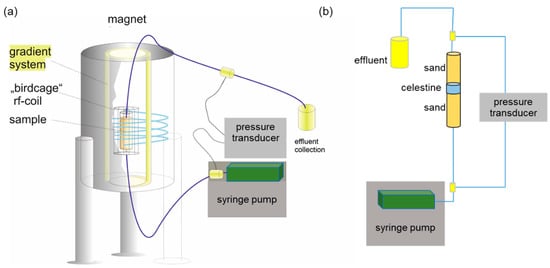
Figure 1.
(a) Schematic representation of the experimental setup with the flow through column placed in a high field magnetic resonance imaging scanner. It is composed of a superconducting magnet, a gradient system for creating magnetic field gradients for imaging in three Cartesian directions, and a radiofrequency coil (200 MHz) for the excitation and detection of the NMR signal. The sample is inserted into the rf-coil, whereas the other components of the setup such as pressure transducer and pump are placed outside to avoid disturbance by the magnet’s stray field. (b) experimental setup for permeability measurements.
After insertion of the sample into the magnet, the system was equilibrated for 24 h by pumping a saturated solution of SrSO4 through the column at a flow rate of 2.5 × 10⁻¹⁰ m−3 s−1. On day zero, the dissolution of celestine and subsequent precipitation of barite was triggered by injection of a 10 mM BaCl2 solution at a flow rate of 2.5 × 10⁻¹⁰ m−3 s−1. The entire reaction was monitored for a period of 30 days with frequent MRI scans (see below Section 3.2). The injection of the BaCl2 solution triggers the dissolution of celestine and subsequently barite precipitation due to the difference in their solubility products (K0sp (BaSO4) = 10−9.97 mol2 L−2 and K0sp(SrSO4) = 10−6.63 mol2 L−2 at 298.15 K and 1013 hPa [46]).
The mineral transformation in the column can be described as follows:
Ba2+(aq) + SrSO4(s) ↔ BaSO4(s) + Sr2+(aq)
Because of the larger molar volume of barite (52.1 cm3 mol−1) compared to celestine (46.25 cm3 mol−1), a porosity and permeability decrease is expected.
The porosity, , of the quartz sand and celestine regions was (0.46 ± 0.02) m3 m−3, evaluated using the following formula:
where ρbulk [kg m−3] and ρgrain [kg m−3] are the bulk and grain densities (measured quantity) of the solid, respectively. Bulk densities were calculated as the ratio of the mass of the quartz/celestine and the volume of the column. The initial and final permeabilities of the system (i.e., comprising both sand layers, the celestine layer, and filters) were determined by differential pressure measurements (see Appendix A). The initial characteristics of the column are summarized in Table 1.

Table 1.
Summary of experimental parameters.
The injection of the BaCl2 solution lasted 30 days to ensure observable changes in the celestine layer. The column effluent was sampled at regular time intervals. The sampled effluents were filtered and their chemical composition determined using ion exchange chromatography for anions (Cl−, SO42−) and by inductively coupled plasma-optical emission spectrometry (ICP-OES) for cations (Sr2+, Ba2+). This enabled the quantification of the amounts of SrSO4 that dissolved and of BaSO4 that precipitated with time, and consequently the net porosity changes of the system. After the experiment, the porous medium in the column was impregnated under vacuum using resin (Araldite), sliced longitudinally and polished for scanning electron microscopy (SEM) investigation. SEM examinations were carried out in low vacuum mode at 60 Pa, using a FEI Quanta 200F electron microscope (Thermo Fischer Scientific, Waltham, MA, USA) equipped with EDS (Apollo X silicon drift Detector, EDAX), to investigate the chemical and microstructural changes in the celestine and sand regions.
3.2. Nuclear Magnetic Resonance Measurements
We monitored the progress of the reaction from SrSO4 to BaSO4 by MRI with so-called relaxation time mapping in a Bruker vertical super wide bore scanner. Its field strength of 4.7 T corresponds to a 1H Larmor frequency of 200 MHz (Figure 1a). The system was equipped with a set-in gradient system with a maximum gradient strength of 1.4 T m−1 and rf probe head with 25 mm internal diameter. T2 relaxation time maps were obtained by a multi-slice multi-echo pulse sequence in vertical orientation with a field of view of 32 × 16 mm, a matrix size of 256 × 128 points, and 12 slices with a thickness of 0.9 mm and a gap of 0.1 mm in interleaved mode. Further, 48 echoes were recorded with an echo time of 2.0 ms and a repetition time of 10 s, sufficiently long to avoid saturation effects due to long T1 times.
For T1 mapping we used a single-echo, multi-slice sequence with inversion recovery (IR) preparation in the same selected axial slices with a thickness 2 mm and a field of view (FOV) of 16 × 16 mm through fresh and reacted domains of the column. Inversion times were varied in 7 steps between tinv = 0.4 s and tinv = 4 s and an additional reference scan was performed without IR preparation. The evaluation proceeded by complex division of the scans with IR preparation by the reference scan. This procedure benefits from the full range of the IR prepared signal from −1 to +1 for the real part of the complex image and the avoidance of cross-talk effects [40]. Additionally, fresh and fully reacted columns were scanned separately to determine the respective T1 and T2 relaxation times. To assess the contribution of internal gradients (see Equation (3)) we also determined the dependence of T2 on tE for the fresh sample. The echo time was varied between 1.6 and 4.0 ms, the slice thickness was 8 mm and the resolution was 32 × 32 points for an isotropic FOV of 16 mm.
All mathematical calculations involved in the image processing, such as fast Fourier transformation, filtering, and complex division, were performed within IDL (Harris Geospatial, Broomfield, CO, USA), for the final graphical representation we used Fiji [47].
3.3. ESR Measurements
ESR measurements were performed to determine the amount of paramagnetic impurities in the porous media by using a benchtop X-band EPR spectrometer Magnettech 5000 (Magnettech, Freiberg Instruments, Freiberg, Germany) at 304 K with the following parameters: modulation amplitude, 1 G; microwave power, 10 mW; microwave frequency, 9.4656 GHz. A DPPH (2,2-diphenyl-1-picrylhydrazyl) reference sample was used to calculate the concentration of paramagnetic centers.
3.4. Assessing Celestine Reactivity due to Barite Overgrowth Using Reactive Transport Tools
A micro-continuum reactive transport model was used to investigate the impacts of the properties of the precipitating barite layer on subsequent celestine dissolution and barite precipitation. Without detailed geometric information, the model considers a flat channel scenario, which is the equivalent of tracking the reactions along the path of a streamline (Figure 2). Three layers of materials are included: the grain of celestine, the barite coating, and the pore fluid. The thickness of the three layers in the model are 25 µm (celestine, cel), 2.5 µm or 5 µm (barite) and 25 µm (pore water, PW), consistent with the grain size of 20–63 µm and a porosity of 0.46 m3 m−3. The length of the computational domain is chosen to be 2 cm, which assumes a tortuosity of 2 in the 1 cm celestine section, to illustrate the variations of upstream and downstream reactions due to reactions along the flow path.
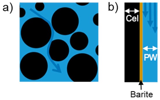
Figure 2.
(a) Schematic of fluid flow in porous media, and (b) a simplified model following a streamline, the so-called flat channel scenario.
The simulations were performed using CrunchFlow [48]. The governing equation is the mass balance equation:
where [m3 pore space m−3 porous medium] is the porosity, and a value of 1 is used for the pore space. No flow is considered in the matrix, and the velocity in the pore water follows a parabolic velocity profile and has an average value of 6.96 × 10⁻⁶ m s−1. is the dispersion tensor, which in this case assumes the value of molecular diffusion in the pore water and an effective diffusivity in the barite precipitate. A range of diffusivity values for the newly formed precipitate (1 × 10⁻⁹, 1 × 10⁻¹⁰, 1 × 10⁻¹¹, 1 × 10⁻¹², 1 × 10⁻¹⁴ m2 s−1) were tested. For the simulations, Equation (8) is written with respective to the total concentrations of H2CO3, Sr2+, Ba2+, SO42−, and Cl−. Concentrations of other aqueous species, e.g. CO32−, are solved based on the total concentrations of the primary species and the law of mass action.
Mineral reactions (, [mol m−3 porous medium s−1]) are treated as a source/sink term.
where is the stoichiometric coefficient of species in the reaction of mineral . [m2 m−3 porous medium] is the reactive surface area, and is calculated based on a specific surface area of 0.077 m2 g−1 assuming the same value for both celestine and barite. Celestine dissolution and barite precipitation are treated kinetically following the transition state theory rate laws:
where [mol m−2 s−1] is the kinetic coefficient [49]. The last term is the chemical affinity that depends on the ion activity product (), the solubility constant (). The ratio of to is termed saturation ratio. This simulation is a sensitivity case study to evaluate the effect of the diffusivity of the barite overgrowth on further barite precipitation and do not account for the evolution of the coating (overgrowth) layer. Rather, we focus on the steady state reaction rate for a given combination of parameters.
4. Results
4.1. Mineral Transformation, Porosity and Permeability Changes
The ingress of the BaCl2 solution triggers the dissolution of celestine leading to the precipitation of barite. Figure 3 shows SEM images of the reacted porous medium from the column experiment, collected at the upstream region and downstream region of the reacted celestine layer. Barite precipitated as an overgrowth on the surface of the celestine, the thickness of the barite overgrowth increased from the upstream region (~2.5 µm rim thickness) to the downstream region (>5 µm rim thickness) of the celestine layer (Figure 3a,b). Based on the SEM images, the amount of barite that precipitated downstream appears higher than the amount that precipitated upstream; this will be further discussed in Section 5.1. No precipitation of barite was observed in the sand region. Previous experimental observations revealed the absence of Ba-Sr-sulfate solid solutions under the chosen experimental conditions [16].
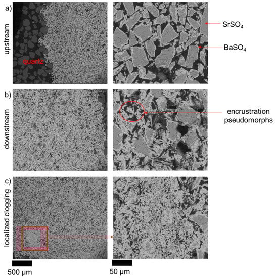
Figure 3.
SEM Back Scattered Electron (BSE) images of the celestine region after 30 days of BaCl2 injection; (a) upstream sand/celestine interface, (b) downstream celestine/sand interface, and (c) zones of localized clogging. The darker shades refer to a Sr rich phase (SrSO4) and the lighter refer to a Ba rich phase (BaSO4).
The mineralogical changes of the porous medium during the flow-through experiment are shown in Figure 4a, calculated from the difference between the composition of the injected solution and that of the effluent. The total celestine dissolution and barite precipitation (in the system) proceeded linearly with time. The global rate of dissolution and consequently precipitation (Figure 3b) were constant at −2.5 × 10⁻⁹ mol s−1 and 2.5 × 10⁻⁹ mol s−1, respectively, for the first 600 h of the experiment and decreased afterwards. This deceleration of the dissolution rate of celestine is due to passivation by barite formed on its surface (cf. Figure 4). Consequently, less SO42− is liberated into the pore space, slowing down the further precipitation of barite.
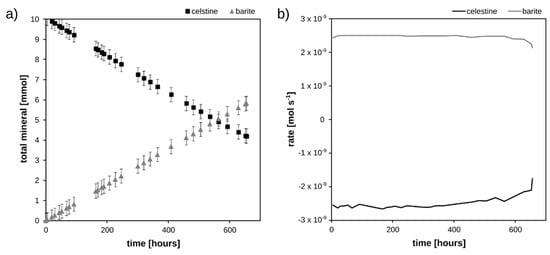
Figure 4.
(a) Total amounts of minerals in the column, and (b) rates of barite precipitation and celestine dissolution as function of time.
The temporal evolution of the bulk porosity of the reactive celestine layer, calculated from the amounts of minerals present and their molar volumes, and the permeability measured before and after the experiment are presented in Figure 5. Throughout the experiment, the overall porosity of the celestine layer decreased only slightly by ~8% from 0.460 m3 m−3 to 0.424 m3 m−3, while the permeability decreased significantly by a factor of ~30. Because of the relatively long tubings (3 m) connecting the column to the pressure transducer (placed outside of the 0.5 mT stray field of the magnet), the recorded pressure measurement during the experiment were not useable and are therefore not presented. The observed porosity and permeability changes are within the same orders of magnitude as reported in previous work for a similar experimental set up and identical boundary conditions [16].
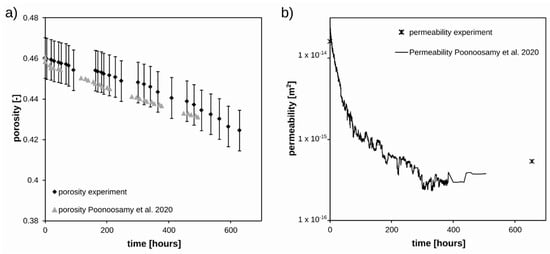
Figure 5.
(a) Calculated porosity, and (b) measured permeability in the celestine layer during the experiment. The measured porosity and permeability changes obtained by Poonoosamy et al. for similar boundary conditions are provided for comparison [16].
4.2. Magnetic Resonance Imaging
MRI allows the reaction front to be observed online and non-invasively while the column remains connected to the pump and pressure transducer. Its contrast is based on the liquid content and the local relaxation properties in the porous medium. We monitored the system under full saturation. Since the change in porosity, i.e., the change in the local liquid content is relatively small, which is also partially related to the S/V parameter in Equation (4), we expect that the change in the mineralogy and the related properties (magnetic susceptibilities) of the pore system will control the contrast by changes in the relaxation times, and consequently the reaction progress is monitorable by MRI relaxation time mapping. The convenience of this approach is illustrated in Figure 6 for the column after eight days of reaction. The longitudinal relaxation times in the reacted zone (at 1 and 3 mm) are not significantly shorter than in the pristine zone at 5 and 7 mm above the lower boundary of the SrSO4 zone (Figure 6b).
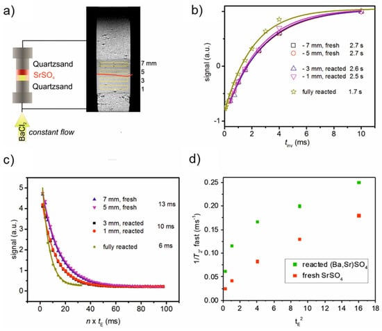
Figure 6.
(a) Setup showing the state on day 8; flow is from bottom. In a central vertical MRI slice the reacted zone is clearly distinguishable from the pristine zone by it’s brighter color. The boundary is indicated by a red curve. Shown are also four selected axial slices at 1, and 3 mm in the reacted zone and at 5 and 7 mm in the pristine zone. (b) T1 relaxation curves in the selected zone plus the curve from a fully reacted sample (after the experiment), separately measured. (c) T2 relaxation curves in the selected zone plus the curve from a fully reacted sample, separately measured. T1 and T2 values were obtained by fitting an exponential function to the data of b) and c) and included. (d) Dependence of 1/T2 of pure celestine and reacted celestine/barite packings as a function of the inter-echo spacing tE2.
Additional measurement on the fully reacted sample showed a slight decrease of T1 (see Figure 6b, green curve). The change in T2 is more significant (Figure 6c). It reduces from 13 ms in the pristine zone to 10 ms in the reacted zone and further to 6 ms when fully reacted (Figure 6c, green curve). Considering Equation (2), the observed constant T1 and reduced T2 suggest a predominance of the relaxation enhancement by water diffusion in internal gradients over the surface-enhanced relaxation acceleration controlled by the pore surface to volume ratio. An obvious explanation are the different magnetic susceptibilities of celestine, −57.9 10−6 cm3 mol−1, and barite, −65.8 10−6 cm3 mol−1 [50]. They are sufficiently different to contribute to significant changes in the third term of Equation (2), which describes the acceleration of transverse relaxation due to diffusion in internal gradients g.
The investigation of the dependence of 1/T2 on the square of the echo time tE (Figure 6d) indicates a strong contribution of accelerated relaxation by diffusion in internal gradients. The initial slopes of the curves in Figure 6d make it possible to estimate the internal gradients according to Equation (3) as 2.2 T m−1 for the reacted sample or 1.0 T m−1 for the fresh sample. These values are in the same order of magnitude as found for washed quartz and natural beach sands [51].
The relaxometry results show that T1 changes only slightly, but T2 becomes significantly shorter and thus allows the progress of the conversion from celestine to barite to be monitored with the help of T2 mapping. Figure 7 shows the temporal evolution of the relaxation time map (T2) as the reaction proceeded. Initially, during the first week, a reaction front developed and moved upwards with relative homogeneous distribution of relaxation times. Later, from day 15 onwards, a clearly heterogeneous distribution of regions with a high degree of conversion (dark blue patches) behind the front also occurred. These localized regions of a few 100 µm2 size correspond to the localized clogging observed in the SEM images (Figure 3c).

Figure 7.
MRI T2 relaxation time maps of a central vertical slice through the column. The reaction started on day 0 and the experiment was terminated on day 30. Flow is from bottom to top. Please note that the color in the sand packing below and above the celestine/barite zone is uniformly red due to overexposure in the selected color table. The excerpt on the right hand side in the bottom line shows exemplary patchy patterns of the barite precipitate. Resolution was 0.125 mm in-plane and the slice thickness was 0.9 mm.
The advancement of the precipitation front, characterized by a decrease of the mean relaxation time (T2), was further analyzed as a function of time (see Figure 8). Generally, the advancement speed of a few mm per week is much slower than the pore flow velocity of 0.6 m per day, which corresponds to an exchange of 59 pore volumes per day. This indicates that the advancement of the precipitation front is not to be confused with a classical break-through curve, which would proceed approximately with the pore flow velocity. Rather, the rate-determining step is the reaction on the mineral surface. Because BaCl2 is supplied at a constant rate, the advancement of the front was surprisingly not linear with time, but was rather a function of the square root of time (√t) indicating a diffusive process. Possible reasons will be discussed in Section 5.1.

Figure 8.
Graph of the advancement of the precipitation front as function of time.
4.3. Empirical Relationships Linking Relaxation Time to Permeability
The effective inverse relaxation times, 1/T2,eff in Equation (2), of the fresh celestine and reacted medium (Figure 6d) allow to estimate the permeability k using empirical relations according to Equations (4) and (5) considering the measured porosities and pore radii. The most widespread classical model of Kenyon relates k to the 2nd power of the average effective relaxation time and the 4th power of porosity. Alternatively, Pape et al. have developed another model, where the permeability scales linearly with the relaxation time and quadratic with the mean pore radius and the porosity [28]. We used both models to estimate the ratio of permeability of unreacted column (pure celestine) and reacted column (celestine and barite) to compare the results with the experimental data taken from Figure 6b; Table 2 gives a summary. Although, the absolute permeability values derived from [28] differ by a factor of 2–4, the experimental ratio of kunreacted/kreacted = 30 is very satisfactorily confirmed by the NMR-based results. The classical mean 1/T2,eff model of Schlumberger-Doll yields a ratio of 12 [35], whereas the model of Pape [28] gives a closer value (20) to the experimentally observed ratio. The obtained surface relaxivities are in the same range as observed for some washed and natural sands [52].
Table 2.
Evaluation of permeabilities and input parameters used for the calculations.
4.4. Numerical Modelling of the Barite Overgrowth
The numerical results reported here are steady state barite overgrowth rates for a given combination of diffusivity and thickness of the coating layer, in order to examine the impacts of coating layer properties on the overgrowth rate of barite. While conditions such as the flow rate and thickness range of the coating layer are taken from the experiments, some of the settings (e.g., geometry) of the sensitivity analyses are simplified and the intent is not to reproduce the experimental observations.
The effective diffusivity of the coating barite layer on the celestine grains can impact the subsequent barite precipitation. Figure 9a shows the barite precipitation rate of a 0.5 mm section at the upstream as a function of the diffusivity of an existing barite layer. Our numerical investigation shows that decreasing the effective diffusivity of the coating layer from 1 × 10⁻⁹ m−2 s−1 to 1 × 10⁻¹¹ m2 s−1 would cause the precipitation rate in the highlighted box to decrease from ~1.6 × 10⁻¹⁴ mol s−1 to ~6.1 × 10⁻¹⁷ mol s−1. At a low diffusivity of 1 × 10⁻¹¹ m2 s−1, no precipitation occurred after 10 h because the outward diffusing SO42− from celestine dissolution and the inward diffusing Ba2+ have not mixed yet. The thickness of the coating layer has a secondary effect on the barite precipitation rate. A thinner coating layer corresponds to a weaker diffusion limitation and thus higher precipitation rate. The precipitation rate in presence of a 2.5 µm coating layer is higher by a factor of ~3 than the rate in presence of a 5 µm coating layer when the diffusivity is 1 × 10⁻⁹ m2 s−1, the factor is ~2 when a diffusivity of 1 × 10⁻¹¹ m2 s−1 is used instead.
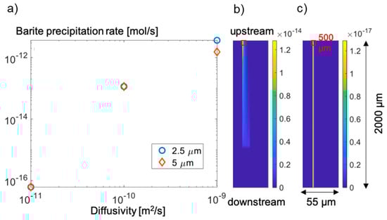
Figure 9.
(a) Barite precipitation rate as a function of the effective diffusivity of the coating layer assuming a thickness of 2.5 µm and 5 µm, (b) barite precipitation rate simulated with a diffusion coefficient of 1 × 10⁻¹⁰ m2 s−1 and a layer thickness of 5 µm leading to high barite precipitation rate and no precipitation downstream, and (c) barite precipitation rate simulated with a diffusion coefficient of 1 × 10⁻¹¹ m2 s−1 and a layer thickness of 5 µm leading to low barite precipitation rate all over the considered section (See also Figure 2). The red box in (b) and (c) highlights the region used to calculate the barite precipitation rate presented in (a).
The effective diffusivity of the coating barite layer also largely influences the difference between the upstream and downstream precipitation rate as schematically shown in Figure 2b. For instance, with a high diffusivity, the precipitation rate is high in the upstream and Ba2+ becomes depleted in the downstream, leading to no precipitation or a low local precipitation rate. This is demonstrated in Figure 9b. In contrast, if the diffusivity is low, the upstream precipitation rate is low, making Ba2+ available for downstream precipitation as well (Figure 9c).
5. Discussion
5.1. Heterogeneous Distribution of Barite Across the Reaction Layer
As expected from the experimental conditions, barite precipitated unevenly across the celestine region. This was explained in by the different supersaturation with respect to barite and consequently differences in the barite nucleation rates that prevail along the celestine region (calculated supersaturation upstream and downstream were 103.82 and 100.34, respectively, cf. Table 3 in [16]. At high supersaturation (saturation ratio > 103), nucleation is fast leading to a rapid precipitation of barite on the celestine, passivating its surface and slowing down its further dissolution. At lower supersaturation (saturation ratio < 103), barite nucleates at a slower pace on the surface of the celestine. Besides, at low supersaturation, the energy barrier to nucleate new barite is more significant than at high supersaturation, which would mean that it is easier to grow on existing barite [53]. This resulted in partial covering of the celestine with a barite coating. Moreover, it enabled further dissolution of the celestine grains and precipitation of barite on the surface, leading to an increase of the barite overgrowth (rim thickness) and formation of encrustation pseudomorphs in some cases.
In addition, we observed localized clogging zones at several places as shown in Figure 3c. These regions show a completely different pore network than the rest of the column. The possible reason for these localized clogging zones could be explained either by an initial heterogeneity, which is unlikely in this case based of the rather homogeneous initial relaxation map reported in Figure 7. These clogging zones might result from the development of local heterogeneities in the celestine region, characterized by lower local porosities and consequently lower flow velocities. It translated into an increase in residence time, favoring a complete dissolution of celestine and precipitation of barite. This line of argumentation is in agreement with the numerical study of Nissan & Berkowitz, who indicated that a low Péclet number (ratio of advective transport time and diffusive transport time) usually increases the amounts of product [54,55].
The description of kinetically controlled dissolution processes in reactive transport models are usually based on a transition state theory (TST) approach with a reactive surface area that usually varies with time. The simplest implemented models, usually scale the reactive surface area linearly to the volume of the dissolving mineral [17]. Alternatively, other more sophisticated models taking into account passivation processes have also been developed [56]. In the passivation model, the reactive surface area is a function of the volumes of the dissolving mineral and of the mineral precipitating as secondary phase on its surface. In an analogous experiment, we observed that for the ingress concentration of 10 mM BaCl2 the dissolution and precipitation scenarios could neither be described by a linearly scaled reactive surface area model for celestine dissolution nor by the passivation model based on Daval et al. [56]. The authors inferred that the barite overgrowth on the surface of celestine was porous and that the porosity/diffusive properties of the barite overgrowth had a major role in further dissolution and precipitation processes [16]. Our current non-invasive monitoring of the progress of the conversion by MRI, showing the dependence of the precipitation front as a function of √t, confirms the hypothesis that the barite overgrowth is porous, and its diffusive properties have to be taken into account. The diffusive properties of this layer is likely to depend on the nucleation rate of barite and thus on the supersaturation that prevails across the celestine region. Our numerical investigation suggests that the diffusive properties of the barite overgrowth could influence further dissolution/precipitation processes. The higher the diffusive properties of the barite overgrowth, the higher is the amount of barite that precipitates and vice versa. The sensitivity analysis gives a hint that the barite overgrowth upstream could have a lower diffusivity than downstream which would translate into a decrease in the dissolution of celestine upstream compared to downstream, increasing the thickness of the barite overgrowth downstream. The variation in diffusivity may be related to the dependence of the precipitation mechanisms on supersaturation, as discussed earlier.
5.2. Porosity/Permeability Changes and Application of MRI Based Empirical Relationships
The barite precipitation in the porous medium altered the net porosity by only −8% but significantly changed the permeability of the system by a factor of 30. In parallel the effective transverse relaxation rates increased by a factor of three. This, at first glance, unexpected behavior might reflect a decrease in pore and pore-throat sizes as shown in the numerical investigations of Steinwinder and Beckingham [21]. In addition, the presence of localized clogging zones (Figure 3) could strongly affect the tortuosity of the system, decreasing also its permeability which is in in agreement with previous observations [16]. In the previous work [16], different porosity/permeability relationships implemented in reactive transport codes were tested against experimental observations to predict the evolution of permeability due to barite precipitation. The porosity/permeability relationship involving a critical porosity (see Appendix B, Equation (A2)), usually defined as the porosity at which the porous media becomes impermeable [19], gave a satisfactory match with experimental observations compared to classical porosity permeability relationships derived from the Kozeny-Carman (see Appendix B Equations (A3) and (A4)). However, the authors had no clear understanding of the physical meaning of the so-called critical porosity, nor experimental evidence of a change in pore connectivity. With the current combination of MRI and SEM results, it is clear that the localized clogging zones substantially changes the pore connectivity. These localized clogging zones with a size in the order of 100 µm are still porous (Figure 3c) and need to be upscaled in a continuum scale-based model. Including a critical porosity could be an elegant way of upscaling these pore scale features.
The changes in the relaxation times observed after 15 days, when first indication of the localized clogging occurs, might indicate changes in the pore architecture. This reorganization of the pore structure might be due to changes in flow velocities, flow field, and pressure as a consequence of the localized clogging, since the solution is pumped at a constant rate.
The strong decrease of permeability is also consistent with permeability models derived from NMR relaxometry, which is a common tool for the assessment of liquid availability in well logging by combination of different experimental information [35]. The conventional (NMR) model of Kenyon, but even better the more elaborated model of Pape et al. reproduced very satisfactorily the observed decrease in permeability from the combination of porosity changes with the decrease in transverse NMR relaxation times. Please note that the empirical factors, characteristic for the chemistry and mineralogy of the given porous medium remained constant. It is reasonable since the system does not change significantly. Both mineral phases represent alkaline earth metal sulfates.
Regarding the NMR relaxation times, the most striking point is the uncommon high ratio of T1/T2 combined with a significant, non-linear dependence of T2 on the square of the echo time. Furthermore, the latter effect became stronger with the conversion of the mineral phases whereas the change in T1 was smaller. Due to the fact that the effective, observable relaxation rates are dominated by internal magnetic field gradients, which generally may result from paramagnetic impurities or inherent magnetic susceptibilities of the mineral phases themselves. To exclude the first factor, we have measured the electron spin resonance of the original SrSO4. The ESR spectrum (Figure 10) allowed the calculation of the mass electron spin density as the 0.17 µmol g−1, which is typical for mineral phases with non-paramagnetic metal ions. The structure of ESR spectrum reflects the presence of paramagnetic centers, which are represented by holes and electron centers of sulfate ions and oxygen radicals [57].
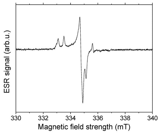
Figure 10.
ESR spectrum of fresh celestine packing.
Thus, the only remaining factor responsible for the accelerated T2 relaxation is the change of the magnetic susceptibility accompanying the conversion from celestine (χ = −57.9 10−6 cm3 mol−1) to barite, (χ = −65.8 × 10⁻⁶ cm3 mol−1). It caused the steeper increase of the transverse relaxation rate with the echo time but also the different offsets when extrapolating to tE = 0 (see also Table 2, Column 7). The high ratio of T1/T2 persists even for the extrapolated values of T2. Since the extrapolation eliminates the influence of the third term (in Equation (2)), we could calculate the specific relaxivities for celestine as 50 µm s−1 and for barite as 60 µm s−1 (Table 2). These data are in the same range as obtained for purified silica sand, where we have found values between 60 and 130 µm s−1 [52]. This significant dependency of T2 on the mineralogy allowed us to observe the reaction progress by MRI with T2 mapping. Here, the observed square-root of time dependence of the reaction front is most probably indirectly due to diffusion processes in the growing barite layer on the celestine grains. Since the progress of the reaction was monitored over a long period, the development of the clogging zones could be detected.
6. Conclusions
In this work, we explored the application of MRI for the assessment of transport parameters (porosity and permeability) and mineralogical changes during barite precipitation in porous media. The NMR results show that the dissolution of celestine followed by the precipitation of barite led to a slight change in the net porosity and the formation of localized clogging zones. The permeability change derived from porosity/permeability relaxometry relationship, in agreement with independent experimental measurements, was substantial, highlighting the impact of the localized clogging zone and pore throat reduction (observed during SEM investigation), which would reduce the pore connectivity. Further work will focus on the investigation of the pore connectivity using low field 2D relaxometry [40].
The temporal and spatial distribution of barite obtained from MRI and SEM as well as the micro-continuum reactive transport model sensitivity analysis suggest that the mineral overgrowth is porous and allows the diffusion of solutes, thus affecting further mineral dissolution and precipitation. Future work will combine TEM work to assess the porosity of the barite overgrowth upstream and downstream, which will be used as input parameter in a “growing core model with a defined diffusivity” as an attempt to describe the heterogeneous distribution of barite in the column. Understanding the interplay between macroscopic flow regimes and microscopic reaction mechanisms (e.g., nucleation and crystal growth pathways) in controlling the dynamic evolution (thickness and diffusive properties) of the coating (overgrowth) layer is still a challenging and unresolved task. This requires further investigation as it has important implications for predicting natural weathering processes, scaling in the subsurface energy production systems, cement degradation, and glass corrosion among others. The combination of pores scale modelling and microstructural information is a versatile tool to investigate these phenomena [58,59].
Author Contributions
J.P., A.P., G.D., F.B. and D.B. participated in the design of the experiment. J.P. and AP. conducted the experiments. A.P. and S.H.-P. analyzed relaxometry measurements. J.P. did the chemical and permeability analysis. H.D. conducted the modelling. M.K. and J.P. conducted the SEM investigations. B.G. and S.S. did the ESR measurements. All authors contributed to the discussion of the results and to writing the manuscript. All authors have read and agreed to the published version of the manuscript.
Funding
The research leading to these results has received funding from the German Federal Ministry of Education and Research (BMBF, grant agreement 02NUK053A) and from the Initiative and Networking Fund of the Helmholtz Association (HGF grant SO-093) within the collaborative project iCross.
Acknowledgments
The first author is indebted towards David Caterina for setting up the contact with Andreas Pohlmeier and for making the first test MRI measurements on her samples. This work beneficiated from the technical support of Daniel Assenmacher. Hang Deng would like to thank the support from the Spent Fuel and Waste Science and Technology Campaign, Office of Nuclear Energy, of the U.S. Department of Energy under Contract Number DE-AC02-05CH11231 with Lawrence Berkeley National Laboratory.
Conflicts of Interest
The authors declare no conflict of interest.
Appendix A
The initial and final permeability of the system (i.e. comprising both sand layers, the celestine layer and filters) were determined by differential pressure measurements during the injection of a solution at a constant flowrate of 2.5 × 10⁻¹⁰ m−3 s−1 during 12 h. For these measurements, a saturated SrSO4 solution (initial measurement) and a saturated BaSO4 solution (final measurement), respectively, were used. Pressure sensors X26-015DV from Omega Engineering Inc., allowing the measurement of pressure differences from 0 to 1030 hPa, were used in our study to measure the permeabilities. The sensitivity of the sensor was 0.1 hPa. The permeability, ktot, was determined using Equation (A1):
where Q is the flow rate [m3 s−1], A [m2] and L [m] are the inner cross sectional area and length of the column, respectively, µ is the fluid viscosity [Pa s] and Δp [Pa] is the difference in pressure between the outlet and inlet. The permeability of the sand was determined independently using the same procedure, i.e. measuring the differential pressure during the time water was pumped in at a constant flow rate of 2.5 × 10⁻¹⁰ m3 s−1 through a 0.07 m long sand column. The permeability of the filter (80 µm thick polyester cloth) was determined using a falling head method [60]. The permeabilities of the filter and the compacted sand were (2.4 ± 0.1) × 10−14 m2 and (8.1 ± 0.1) × 10−12 m2, respectively. The initial permeability of the celestine layer was calculated from the permeabilities determined for the complete system and the data for the sand layers and filters, respectively, to (1.55 ± 0.6) × 10−14 m2, following the approach that the overall permeability of a layered system can be represented by the harmonic mean of the permeabilities of the individual layers [61].
ktot = (µLQ)/(AΔp)
Appendix B
Empirical formulations based on the Kozeny-Carman, parameterizing the complex evolution of the pore space geometry to porosity changes as the only parameter (Equations (A2) and (A3)) and commonly used in numerical models.
Verma and Pruess proposed a porosity-permeability relationship as follows [62]:
where k0 and are the initial permeability and porosity respectively. and n are the critical porosity and the exponent with the general relation; , for . The critical porosity of a porous medium refers to the porosity at which the medium becomes practically impermeable.
References
- Poonoosamy, J.; Wanner, C.; Alt Epping, P.; Aguila, J.F.; Samper, J.; Montenegro, L.; Xie, M.; Su, D.; Mayer, K.U.; Mäder, U.; et al. Benchmarking of reactive transport codes for 2D simulations with mineral dissolution/precipitation reactions and feedback on transport parameters. Comput. Geosci. 2018, 1–22. [Google Scholar] [CrossRef]
- Xie, M.L.; Mayer, K.U.; Claret, F.; Alt-Epping, P.; Jacques, D.; Steefel, C.; Chiaberge, C.; Simunek, J. Implementation and evaluation of permeability-porosity and tortuosity-porosity relationships linked to mineral dissolution-precipitation. Comput. Geosci. 2015, 19, 655–671. [Google Scholar] [CrossRef]
- Fu, Y.J.; van Berk, W.; Schulz, H.M. Hydrogeochemical modelling of fluid-rock interactions triggered by seawater injection into oil reservoirs: Case study Miller field (UK North Sea). Appl. Geochem. 2012, 27, 1266–1277. [Google Scholar] [CrossRef]
- Oddo, J.E.; Tomson, M.B. Why scale forms and how to predict it. SPE Prod. Facil. 1994, 9, 47–54. [Google Scholar] [CrossRef]
- Aquilina, L.; Dia, A.N.; Boulègue, J.; Bourgois, J.; Fouillac, A.M. Massive barite deposits in the convergent margin off Peru: Implications for fluid circulation within subduction zones. Geochim. Cosmochim. Acta 1997, 61, 1233–1245. [Google Scholar] [CrossRef]
- Mundhenk, N.; Huttenloch, P.; Sanjuan, B.; Kohl, T.; Steger, H.; Zorn, R. Corrosion and scaling as interrelated phenomena in an operating geothermal power plant. Corros. Sci. 2013, 70, 17–28. [Google Scholar] [CrossRef]
- Vengosh, A.; Jackson, R.B.; Warner, N.; Darrah, T.H.; Kondash, A. A critical review of the risks to water resources from unconventional shale gas development and hydraulic fracturing in the United States. Environ. Sci. Technol. 2014, 48, 8334–8348. [Google Scholar] [CrossRef]
- Vinograd, V.L.; Kulik, D.A.; Brandt, F.; Klinkenberg, M.; Weber, J.; Winkler, B.; Bosbach, D. Thermodynamics of the solid solution-Aqueous solution system (Ba,Sr,Ra)SO4 + H2O: II. Radium retention in barite-type minerals at elevated temperatures. Appl. Geochem. 2018, 93, 190–208. [Google Scholar] [CrossRef]
- Klinkenberg, M.; Weber, J.; Barthel, J.; Vinograd, V.; Poonoosamy, J.; Kruth, M.; Bosbach, D.; Brandt, F. The solid solution-aqueous solution system (Sr,Ba,Ra)SO4 + H2O: A combined experimental and theoretical study of phase equilibria at Sr-rich compositions. Chem. Geol. 2018, 497, 1–17. [Google Scholar] [CrossRef]
- Brandt, F.; Klinkenberg, M.; Weber, J.; Poonoosamy, J.; Bosbach, D. The effect of ionic strength and Sr-aq upon the uptake of Ra during the recrystallization of barite. Minerals 2018, 8, 502. [Google Scholar] [CrossRef]
- Poonoosamy, J.; Kosakowski, G.; Van Loon, L.R.; Mäder, U. Dissolution-precipitation processes in tank experiments for testing numerical models for reactive transport calculations: Experiments and modelling. J. Contam. Hydrol. 2015, 177, 1–17. [Google Scholar] [CrossRef]
- Poonoosamy, J.; Curti, E.; Kosakowski, G.; Grolimund, D.; Van Loon, L.R.; Mäder, U. Barite precipitation following celestite dissolution in a porous medium: A SEM/BSE and mu-XRD/XRF study. Geochim. Cosmochim. Acta 2016, 182, 131–144. [Google Scholar] [CrossRef]
- Rajyaguru, A.; L’Hôpital, E.; Savoye, S.; Wittebroodt, C.; Bildstein, O.; Arnoux, P.; Detilleux, V.; Fatnassi, I.; Gouze, P.; Lagneau, V. Experimental characterization of coupled diffusion reaction mechanisms in low permeability chalk. Chem. Geol. 2019, 503, 29–39. [Google Scholar] [CrossRef]
- Vankeuren, A.N.P.; Hakala, J.A.; Jarvis, K.; Moore, J.E. Mineral reactions in shale gas reservoirs: Barite scale formation from reusing produced water as hydraulic fracturing fluid. Environ. Sci. Technol. 2017, 51, 9391–9402. [Google Scholar] [CrossRef]
- Stack, A.G. Precipitation in pores: A geochemical frontier. Rev. Miner. Geochem. 2015, 80, 165–190. [Google Scholar] [CrossRef]
- Poonoosamy, J.; Klinkenberg, M.; Deissmann, G.; Brandt, F.; Bosbach, D.; Mäder, U.; Kosakowski, G. Effects of solution supersaturation on barite precipitation in porous media and consequences on permeability: Experiments and modelling. Geochim. Cosmochim. Acta 2020, 270, 43–60. [Google Scholar] [CrossRef]
- Cochepin, B.; Trotignon, L.; Bildstein, O.; Steefel, C.I.; Lagneau, V.; Van der Lee, J. Approaches to modelling coupled flow and reaction in a 2D cementation experiment. Adv. Water Resour. 2008, 3, 1540–1551. [Google Scholar] [CrossRef]
- Chapuis, R.P.; Aubertin, M. On the use of the Kozeny-Carman equation to predict the hydraulic conductivity of soils. Can. Geotech. J. 2003, 40, 616–628. [Google Scholar] [CrossRef]
- Hommel, J.; Coltman, E.; Class, H. Porosity-permeability relations for evolving pore space: A review with a focus on (bio-)geochemically altered porous media. Transp. Porous Media 2018, 124, 589–629. [Google Scholar] [CrossRef]
- Beckingham, L.E.; Peters, C.A.; Um, W.; Jones, K.W.; Lindquist, W.B. 2D and 3D imaging resolution trade-offs in quantifying pore throats for prediction of permeability. Adv. Water Resour. 2013, 62, 1–12. [Google Scholar] [CrossRef]
- Steinwinder, J.; Beckingham, L.E. Role of pore and pore-throat distributions in controlling permeability in heterogeneous mineral dissolution and precipitation scenarios. Water Resour. Res. 2019, 55, 5502–5517. [Google Scholar] [CrossRef]
- Seigneur, N.; Mayer, K.U.; Steefel, C.I. Reactive transport in evolving porous media. Rev. Miner. Geochem. 2019, 85, 197–238. [Google Scholar] [CrossRef]
- Bray, J.M.; Lauchnor, E.G.; Redden, G.D.; Gerlach, R.; Fujita, Y.; Codd, S.L.; Seymour, J.D. Impact of mineral precipitation on flow and mixing in porous media determined by microcomputed tomography and MRI. Environ. Sci. Technol. 2017, 51, 1562–1569. [Google Scholar] [CrossRef] [PubMed]
- Britton, M.M. MRI of chemical reactions and processes. Prog. Nucl. Mag. Res. Sp. 2017, 101, 51–70. [Google Scholar] [CrossRef]
- Gladden, L.F.; Sederman, A.J. Magnetic Resonance Imaging and velocity mapping in chemical engineering applications. In Annual Review of Chemical and Biomolecular Engineering; Prausnitz, J.M., Ed.; Annual Reviews: Palo Alto, CA, USA, 2017; Volume 8, pp. 227–247. [Google Scholar]
- Pini, R.; Joss, L. See the unseen: Applications of imaging techniques to study adsorption in microporous materials. Curr. Opin. Chem. Eng. 2019, 24, 37–44. [Google Scholar] [CrossRef]
- Sham, E.; Mantle, M.D.; Mitchell, J.; Tobler, D.J.; Phoenix, V.R.; John, M.L. Monitoring bacterially induced calcite precipitation in porous media using magnetic resonance imaging and flow measurements. J. Contam. Hydrol. 2013, 152, 35–43. [Google Scholar] [CrossRef]
- Pape, H.; Arnold, J.; Pechnig, R.; Clauser, V.; Talnishnikh, E.; Anferova, S.; Blümich, B. Permeability prediction for low porosity rocks by mobile NMR. Pure Appl. Geophys. 2009, 166, 1125–1163. [Google Scholar] [CrossRef]
- Carr, H.Y.; Purcell, E.M. Effects of diffusion on free precession in Nuclear Magnetic Resonance experiments. Phys. Rev. 1954, 94, 630–638. [Google Scholar] [CrossRef]
- Meiboom, S.; Gill, D. Modified spin-echo method for measuring nuclear relaxation times. Rev. Sci. Instrum. 1958, 29, 688–691. [Google Scholar] [CrossRef]
- Park, H.W.; Cho, M.H.; Cho, Z.H. Real value representation in inversion recovery NMR imaging by use of a phase-correction method. Magn. Reson. Med. 1986, 3, 15–23. [Google Scholar] [CrossRef] [PubMed]
- Wehrli, F.W.; MacFall, J.R.; Shutts, D.; Breger, R.; Herfkens, R.J. Mechanisms of contrast in NMR imaging. J. Comput. Assist. Tomogr. 1984, 8, 369–380. [Google Scholar] [CrossRef] [PubMed]
- Hurlimann, M.D. Effective gradients in porous media due to susceptibility differences. J. Magn. Reson. 1998, 131, 232–240. [Google Scholar] [CrossRef] [PubMed]
- Kleinberg, R.L.; Kenyon, W.E.; Mitra, P.P. Mechanism of NMR relaxation of fluids in rocks. J. Magn. Reson. A 1994, 108, 206–214. [Google Scholar] [CrossRef]
- Coates, G.R.; Xiao, L.; Prammer, M.G. NMR Logging: Principles and Applications; Halliburton Energy Services: Houston, TX, USA, 1999; 234p. [Google Scholar]
- Mitchell, J.; Chandrasekera, T.C.; Gladden, L.F. Obtaining true transverse relaxation time distributions in high-field NMR measurements of saturated porous media: Removing the influence of internal gradients. J. Chem. Phys. 2010, 132, 244705. [Google Scholar] [CrossRef]
- Blümich, B. NMR Imaging of Materials; Oxford University Press: Oxford, UK, 2003; 568p. [Google Scholar]
- Callaghan, P.T. Principles of Nuclear Magnetic Resonance Microscopy; Clarendon Press: Oxford, UK, 1991; 516p. [Google Scholar]
- Song, Y.Q. Magnetic resonance of porous media (MRPM): A perspective. J. Magn. Reson. 2013, 229, 12–24. [Google Scholar] [CrossRef]
- Haber-Pohlmeier, S.; Vanderborght, J.; Pohlmeier, A. Quantitative mapping of solute accumulation in a soil-root system by Magnetic Resonance Imaging. Water Resour. Res. 2017, 53, 7469–7480. [Google Scholar] [CrossRef]
- Edzes, H.T.; van Dusschoten, D.; Van As, H. Quantitative T-2 imaging of plant tissues by means of multi-echo MRI microscopy. Magn. Reson. Imaging 1998, 16, 185–196. [Google Scholar] [CrossRef]
- Kleinberg, R.L. Well Logging. In Encyclopedia of NMR; Harris, R.K., Wasylishen, R., Eds.; John Wiley & Sons: New York, NY, USA, 1996; pp. 4960–4969. [Google Scholar]
- Sen, P.N.; Straley, C.; Kenyon, W.E.; Whittingham, M.S. Surface-to-Volume ratio, charge density, nuclear magnetic relaxation, and permeability in clay-bearing sandstones. Geophysics 1990, 55, 61–69. [Google Scholar] [CrossRef]
- Vogeley, J.R.; Moses, C.O. 1H NMR relaxation and rock permeability. Geochim. Cosmochim. Acta 1992, 56, 2947–2953. [Google Scholar] [CrossRef]
- Kenyon, W.E. Nuclear Magnetic Resonance as a petrophysical measurement. Nucl. Geophys. 1992, 6, 153–171. [Google Scholar]
- Hummel, W.; Berner, U.; Curti, E.; Pearson, F.J.; Thoenen, T. Nagra/PSI chemical thermodynamic data base 01/01. Radiochim. Acta 2002, 90, 805–813. [Google Scholar] [CrossRef]
- Schindelin, J.; Arganda-Carreras, I.; Frise, E.; Kaynig, V.; Longair, M.; Pietzsch, T.; Preibisch, S.; Rueden, C.; Saalfeld, S.; Schmid, B.; et al. Fiji: An open-source platform for biological-image analysis. Nat. Methods 2012, 9, 676–682. [Google Scholar] [CrossRef] [PubMed]
- Steefel, C.I.; Appelo, C.A.J.; Arora, B.; Jacques, D.; Kalbacher, T.; Kolditz, O.; Lagneau, V.; Lichtner, P.C.; Mayer, K.U.; Meeussen, J.C.L.; et al. Reactive transport codes for subsurface environmental simulation. Comput. Geosci. 2015, 19, 445–478. [Google Scholar] [CrossRef]
- Palandri, J.L.; Kharaka, Y.K. Ferric iron-bearing sediments as a mineral trap for CO2 sequestration: Iron reduction using sulfur-bearing waste gas. Chem. Geol. 2005, 217, 351–364. [Google Scholar] [CrossRef]
- Rumble, J. (Ed.) CRC Handbook of Chemistry and Physics, 100th ed.; CRC Press: Boca Raton, FL, USA, 2019; 1700p. [Google Scholar]
- Washburn, K.E.; Eccles, C.D.; Callaghan, P.T. The dependence on magnetic field strength of correlated internal gradient relaxation time distributions in heterogeneous materials. J. Magn. Reson. 2008, 194, 33–40. [Google Scholar] [CrossRef]
- Duschl, M.; Galvosas, P.; Brox, T.I.; Pohlmeier, A.; Vereecken, H. In situ determination of surface relaxivities for unconsolidated sediments. Water Resour. Res. 2015, 51, 6549–6563. [Google Scholar] [CrossRef]
- De Yoreo, J.J.; Vekilov, P.G. Principles of crystal nucleation and growth. Rev. Miner. Geochem. 2003, 54, 57–93. [Google Scholar] [CrossRef]
- Nissan, A.; Berkowitz, B. Anomalous transport dependence on Peclet number, porous medium heterogeneity, and a temporally varying velocity field. Phys. Rev. E 2019, 99, 33108. [Google Scholar] [CrossRef]
- Nissan, A.; Berkowitz, B. Reactive transport in heterogeneous porous media under different Peclet numbers. Water Resour. Res. 2019, 55, 10119–10129. [Google Scholar] [CrossRef]
- Daval, D.; Martinez, I.; Corvisier, J.; Findling, N.; Goffé, B.; Guyo, F. Carbonation of Ca-bearing silicates, the case of wollastonite: Experimental investigations and kinetic modeling. Chem. Geol. 2009, 265, 63–78. [Google Scholar] [CrossRef]
- Rushdi, M.A.H.; Abdel-Fattah, A.A.; Sherif, M.M.; Soliman, Y.S.; Mansour, A. Strontium sulfate as an EPR dosimeter for radiation technology application. Radiat. Phys. Chem. 2015, 106, 130–135. [Google Scholar] [CrossRef]
- Poonoosamy, J.; Westerwalbesloh, C.; Deissmann, G.; Mahrous, M.; Curti, E.; Churakov, S.V.; Klinkenberg, M.; Kohlheyer, D.; von Lieres, E.; Bosbach, D.; et al. A microfluidic experiment and pore scale modelling diagnostics for assessing mineral precipitation and dissolution in confined spaces. Chem. Geol. 2019, 528, 119264. [Google Scholar] [CrossRef]
- Prasianakis, N.I.; Curti, E.; Kosakowski, G.; Poonoosamy, J.; Churakov, S.V. Deciphering pore-level precipitation mechanisms. Sci. Rep. 2017, 7, 13765. [Google Scholar] [CrossRef] [PubMed]
- Kresic, N. Hydrogeology and Groundwater Modeling, 2nd ed.; CRC Press: Boca Raton, FL, USA, 2006; 828p. [Google Scholar]
- Ahmed, T. Working Guide to Reservoir Rock Properties and Fluid Flow; Gulf Professional Publishing: Burlington, MA, USA, 2010; 262p. [Google Scholar]
- Verma, A.; Pruess, K. Thermohydrological conditions and silica redistribubution near high level nuclear waste emplaced in saturated geological formation. J. Geophy. Res. 1988, 93, 1159–1173. [Google Scholar] [CrossRef]
© 2020 by the authors. Licensee MDPI, Basel, Switzerland. This article is an open access article distributed under the terms and conditions of the Creative Commons Attribution (CC BY) license (http://creativecommons.org/licenses/by/4.0/).