Production Allocation: Rosetta Stone or Red Herring? Best Practices for Understanding Produced Oils in Resource Plays

Abstract

The production of crude oil from resource plays has increased enormously over the past decade. In the USA, around 63% of total output in 2019 was from unconventional production. The major unconventional plays in the USA (e.g., Permian Basin, Anadarko Basin, Eagle Ford, etc.) have become some of the world’s largest oil producers. However, unlike “conventional” exploitation, the target zones in unconventional systems are generally the source rocks themselves or adjacent strata and require numerous horizontal wells and stimulation via hydraulic fracturing to meet production targets. In order to maximize production, operators have developed various well stacking methods, all of which require some form of monitoring to ensure that well spacing is optimized and fluid production is not being “stolen” from adjacent formations, thereby reducing the production potential in associated wells. This necessity, amongst other geochemical considerations related to source rock characterization, has resulted in the expansion of “production allocation” and “time lapse geochemistry” methods. These methods were initially developed for conventional production decades ago, but have since been adapted to unconventional systems. However, the direct applicability of this method is not straightforward and numerous considerations need to be taken into account, foremost among which are: (1) “What defines your end-members?” (2) “Are these end-members valid across a meaningful development area?” and (3) “What is the most appropriate use of geochemistry data in these systems?”. Reservoir geochemistry studies, which include both “time lapse geochemistry/production monitoring” and “production allocation”, are valuable geochemical methods in unconventional plays but need to be used appropriately to provide the cost savings and business direction that operators expect. In this paper, we will discuss a number of case studies, both theoretical and natural, and outline the important factors which need to be considered when designing a reservoir geochemistry study and the common pitfalls which exist. The case studies and best practice approach discussed are designed to highlight the power and flexibility of geochemical data collection methods, integration with the operator’s knowledgebase, and other analytical methods to customize the program for individual development programs. Emphasis is placed upon developing robust and applicable fluid relationships from geochemical data and evidence for statistically significant changes through time.

1. Introduction

Unconventional petroleum systems and production methods, particularly in the USA, have contributed an increasing share of oil production over the past decade. Unlike conventional production methods, where vertical wells primarily target migrated fluids trapped in porous reservoir formations, unconventional production involves targeting the source (or near source) directly via horizontal wells which extend laterally (Figure 1A), potentially for several miles [1,2]. These target formations/zones contain oil locked in tight, low permeability lithologies, and in order to generate economic production, the wells need to be stimulated via hydraulic fracturing. The process of hydraulic fracturing creates what is referred to as a “stimulated rock volume” (SRV) across which the oil flows and allows the oil to be produced (Figure 1B). It has been observed that not all of the stimulated area is actually contributing to production and that the zone from which the oil drains is smaller than the SRV and may change over time as the frac “heals”. This smaller area that directly contributes is referred to as the “drained rock volume” (DRV) (Figure 1B). DRV is what geochemists are ultimately looking to define from produced fluids, whereas SRV is determined by core extracts and methods such as micro-seismic, completion models, and other techniques [3,4].

Another aspect of defining the DRV and the “reach” of production is how many potential contributing zones are being accessed by a single horizontal well. The major unconventional plays in the USA (e.g., Permian, Anadarko, Eagle Ford, etc.) include multiple unconventional target source formations. These formations are generally stratigraphically layered and therefore offer the potential for fluid co-mingling, which can occur over geologic timescales but also created as a result of stimulation during the completion process.

As operators have developed these unconventional assets, understanding the distribution of the SRV to DRV has become increasingly crucial to determining output and the lifetime of individual wells. Ideally, the objective is to maximize production within individual target zones (flow units) without causing interference with nearby wells. Geochemistry aids this understanding by assessing the produced fluid from wells post completion, and adjusting completion strategies for new wells based upon this information. To do this, operators must ask two important questions of the fluid geochemistry data:

• How is the chemistry of the fluid changing through production time (time lapse geochemistry/production monitoring)?
• Which in-situ fluids are contributing to the production fluid (production allocation)?

Question 1 is relatively straightforward and is the premise behind the unconventional time lapse geochemistry studies reported by numerous workers [5,6,7]. Question 2 is a significantly more complicated one to answer, and while there are a number of studies which address this capability [8,9,10,11,12,13], it is certainly not a one size fits all strategy with numerous caveats which will be discussed throughout this paper.

The term production allocation, in respect to petroleum geochemistry, was developed more than 30 years ago in conventional petroleum systems [10,14,15]. Production allocation in conventional systems involves two very crucial pieces of information which are generally lacking in unconventional plays. First, the geochemists have access to definitive end-member fluids which are directly equivalent and comparable to the mixed fluids being assessed. Second, these systems can be considered largely homogenous and, therefore, when quantifying allocation values, error propagation will be low, with a tolerance usually better than 5%. In contrast, unconventional systems are not homogenous. Added to this, the stimulation process further disrupts the homogeneity of the system, and fluid analyses completed prior to stimulation and production becomes irrelevant compared to the produced fluid geochemical data. This means defining an equivalent end-member for produced fluid is challenging to say the least, and the error tolerance will be much greater than that in conventional allocation estimates.

Some studies that allocate production fluids back to specific target formations have utilized extracts from core material (sometimes cuttings) from target formations and have assumed that these extracts are representative of produced fluid end-members [5,16]. However, ignoring cuttings, which have their own considerable issues in terms of provenance and contamination, the extraction of fluids from core material, whether it be via solvents, heat, supercritical CO₂ or some other method, does not mimic the geologic processes which produce oil [17,18,19]. Therefore, while these samples may be incredibly important for core-to-oil correlation studies [20,21,22], their utility as viable fluid end-members for allocation is limited. However, if we were to ignore this and assume the produced and extracted fluids were directly equivalent to one another, we would still have a number of other issues to overcome for these fluids to be useful for quantification. The overriding problem is heterogeneity. Numerous studies (including this one) have shown that, within well-defined and discrete target formations, geochemical heterogeneity exists both stratigraphically and laterally [11,23,24]. A decision must therefore be made as to how to select an extracted fluid that is most representative of the produced fluid:

• the average
• the median
• the closest sample to the target lateral
• the most distinct geochemically, etc.

With all of these potential candidates there are no wrong answers, but there are also no uniquely right answers either.

With few projects containing core from more than one well, yet most laterals being several miles in length, there is a largely unknowable geological/geochemical variability across the SRV in these projects. All of these unknowns suggest that the use of even the best-preserved core material requires caution when it comes to contemplating quantified production allocation in unconventional systems. That is not to say that quantitative allocation is an impossibility. Indeed, generating contribution values is mathematically straightforward, as discussed below. However, there are more appropriate and reliable methods for geochemically assessing fluids to understand contributions and changes through time. Recent studies that understand the above caveats have focused on establishing core-to-oil correlations and used this knowledge to define produced oil end-members (not extracts) and generate realistic allocation thresholds [25].

In this paper, we will use relevant examples to discuss the benefits and limitations of reservoir geochemistry monitoring in unconventional systems. We will present a series of results from projects in the Delaware Basin and the Eagle Ford Play as well as an in-house series of fluid mixing experiments.

2. Methods

2.1. Geochemical Methods

The geochemical data discussed throughout this paper were all collected in GeoMark Research’s organic geochemistry laboratories in Houston, TX, USA. The case studies discussed in this paper followed slightly different analytical programs based largely upon the thermal maturity of the samples and therefore whether traditional biomarkers would be present. All of the samples discussed were analyzed for their bulk properties, specifically API gravity, weight % sulfur, saturate/aromatic/resin/asphaltene (SARA) content, and carbon isotopes (δ¹³C_VPDB) of the saturate, aromatic, and whole oil components. API gravity was measured on 1–2 mL of whole oil via injection into an Anton Paar DMA 500 density meter (Anton Paar GmbH, Graz, Austria) and calculated using the standard API gravity 60 °F method. The weight % sulfur and carbon isotope (δ¹³C_VPDB) signatures were analyzed on a vario ISOTOPE select cube elemental analyzer (EA) connected to a VisION isotope ratio mass spectrometer (IRMS) from elementar (Elementar UK Ltd., Stockport, UK). Weight % sulfur was determined from the thermal conductivity detector (TCD) on the EA and calibrated using known weight % sulfur standards. The carbon isotope results were determined from the IRMS and calibrated to VPDB using known international and in-house carbon isotope standards, including USGS 24 and NBS 22. SARA composition is determined via gravity-flow column chromatography employing a 100–200 mesh silica gel. The samples are deasphaltened using excess n-hexane to determine asphaltene content before hexane is used to elute the saturated fraction, methylene chloride for the aromatic fraction, and a mixture of methylene chloride/methanol for the resin/NSO fraction. Core material discussed in this paper was analyzed following the same procedures, with the exception of API gravity where insufficient volume is generated. Hydrocarbons were extracted from core material using a Dionex ASE 350 (Thermo Fisher Scientific, Waltham, MA, USA) using dichloromethane (DCM) solvent. These extract samples were taken to dryness and quantified prior to be analyzed for their C15+ bulk properties.

All of the samples discussed were also analyzed via high resolution gas chromatography (HRGC) on an Agilent 7890A (Agilent Technologies, Santa Clara, CA, USA) gas chromatograph. Whole oil samples are dissolved in carbon disulfide (CS2) and an internal standard (1-hexene) and injected in split mode (50:1) onto a 50 m × 0.2 μm HP Pona column (0.50 μm film thickness). The GC method is a ramped temperature program with the eluting peaks collected on a flame ionization (FID) detector. HRGC includes peak height and area results as well as peak ratios from both the heavy range of the chromatography (i.e., pristane/phytane) and the gasoline or light hydrocarbon (LHC) range (<nC₉). Hydrocarbon extract samples are analyzed using the sample method on the GC, but are extracted from core chips using a CS2 solvent method while being kept chilled at all times to maximize LC sample integrity [17,19]. Gas chromatography/mass spectrometry (GC/MS) was carried out on the branched/cyclic component of the saturated fraction and on the aromatic fraction. This analytical tool was not used to assess the samples from the Eagle Ford Play, case study 3 in this paper, due to the high maturity of the samples resulting in negligible if any traditional biomarker peak retention. The samples from case studies 1 and 2 were analyzed via this method using an Agilent 7890B GC interfaced to either a 5975C or 5977A mass spectrometer (Agilent Technologies, Santa Clara, CA, USA). The mass spectrometer is run in selected ion mode (SIM) monitoring ions m/z 177, 191, 205, 217, 218, 221, 231, and 259 (branched/cyclic) and m/z 133, 156, 170, 178, 184, 188, 192, 198, 231, 239, 245, and 253 (aromatics). In order to determine absolute concentrations of individual biomarkers, a deuterated internal standard (d4-C29 20R Ethylcholestane; Chiron Laboratories, Norway) is added to the C15+ branched/cyclic hydrocarbon fraction and a deuterated anthracene standard (d10) is added to the aromatic hydrocarbon fraction [20].

2.2. Statistical Methods

All of the geochemical data discussed in this paper were compared using the Pirouette^® statistical software package from Infometrix (Infometrix, Bothwell, WA, USA, Version 4.5 Rev. 1). The three algorithms utilized in this study were hierarchical cluster analysis (HCA), principal component analysis (PCA), and alternating least squares (ALS).

HCA is a statistical algorithm which is used to group similar samples into clusters. In the petroleum industry these clusters are referred to by a number of names, including tribes and families, although all of these terms really refer back to the cluster definition in HCA [15,17,18,20]. Each cluster of samples share similar characteristics, and in this scenario geochemical parameters, which distinguishes them from other clusters of samples. The actual number of clusters are defined by the “user” depending upon the correlation coefficient value selected. The primary visual output from HCA is a cluster dendrogram whereby the samples forming the clusters and their proximity to other samples/clusters is readily identifiable. The HCA dendrograms discussed in this paper are generated from biomarker and isotopic ratios (δ¹³C_VPDB) with the exact parameters utilized varying between projects [15,18,20].

The PCA algorithm is closely associated with HCA and both are generally generated from the same geochemical variables but, while HCA allows clustering of samples to be quickly identified PCA allows the variables controlling those clusters and the separation to be much more readily understood. PCA is an algorithm which reduces the dimensionality of a dataset down to a set of principal components designed to increase interpretability while minimizing information loss. PCA factors (1, 2, 3, etc.) are defined by the relationship between variables rather than by single variables themselves. The primary visual output from PCA is scores, which is the distribution of the samples relative to one another, and loadings, which is the distribution of the geochemical variables. PCA plots can be viewed in 2 or 3 dimensions and are generally color coded relative to the clusters defined by the correlation coefficient selection in the HCA. The HCA and PCA algorithms are generally used together to understand sample relationships and what controls said relationships [20].

The ALS algorithm is a blind source statistical algorithm that is generally utilized, in petroleum geochemistry, to determine the number of “unique” geochemical sources within a given dataset [15]. Additionally, this algorithm allows the contributions of these sources to be determined in geochemically mixed samples. As with the other algorithms, ALS requires geochemical loadings to be input in order to determine source and mixing relationships. However, care needs to be taken when deciding on the appropriate loadings and applying this algorithm as ratio relationships are non-linear [18]. The utility and caveats associated with this specific algorithm are discussed in detail in case study 1 in Section 3.

3. Results and Discussion

The results and discussion section focuses on three components: (1) What do idealized reservoir geochemistry/allocation results look like? (2) What happens when we look to real world examples? (3) Based upon these examples, what are the best practice recommendations for designing such a study? The natural world examples cover two major unconventional plays in the USA (Permian Basin and South Texas Eagle Ford Play) and explain, in detail, the considerations which must be borne in mind when determining the objectives of these studies.

3.1. A Perfect World: In-House Mixing Experiments & Allocation

As discussed in the introduction, reservoir geochemistry projects focused on production allocation is at a disadvantage when applied to unconventional systems. Not only do these systems lack accessible and representative pre-production “end-members” but there is also a significant question over their lateral, and stratigraphic, homogeneity within discrete benches [5,18,26]. However, for the purposes of detailing what can be achieved through this methodology, let’s assume a perfect world with none of these limitations. In order to test the ability to perform production allocation in a perfect system, three distinct end-member oils were selected and mixes were prepared by volume in the laboratory. The geochemical results were then analyzed statistically to test the ability of the un-mixing algorithm in the Pirouette software from Infometrix to match the known amounts.

Three distinct oil samples were selected from GeoMark’s oil library, specifically samples from the Upper Devonian Bakken (1), Miocene Monterey (2), and Cretaceous Tuscaloosa (3) formations, as our end-members (

Table 1. Comparison table of the calculated source contributions relative to the known contributions for both the primarily compositional loadings (A) and the ratio loadings (B). The known end-member oils are highlighted in yellow (Tuscaloosa (T), Monterey (M) and Bakken (B)) as are the known mixed contributions by volume. The percentage offset from this known value as determined from ALS, for compositional loadings (A) and ratios loadings (B) are shown. Calculated contributions greater than 5% from the known mixed value are highlighted in red. Compositional loadings included 15 peaks selected from the collected high resolution gas chromatography (HRGC) and gas chromatography mass spectrometry (GC-MS) results as well as Pr/Ph and Whole Oil δ¹³C_VPDB. Ratio loadings included 18 GC-MS biomarker and isotope ratios.

	Known Mixed Volume + End-Members		(A) ALS Comp Offset			(B) ALS Ratio Offset
Sample ID	End-Members	Volume Mixing	Oil 1 (T)	Oil 2 (M)	Oil 3 (B)	Oil 1 (T)	Oil 2 (M)	Oil 3 (B)
CDB0001	100% Tuscaloosa (T)	100% T; 0% M; 0% B	1%	−1%	0%	2%	−2%	0%
CDB0004		90% T; 10% M; 0% B	2%	−1%	−1%	41%	−41%	0%
CDB0003		80% T; 20% M; 0% B	−10%	10%	0%	46%	−46%	0%
CDB0009		60% T; 40% M; 0% B	−5%	5%	0%	36%	−36%	0%
CDB0002		50% T; 50% M; 0% B	−3%	3%	0%	23%	−23%	0%
CDB0007		40% T; 60% M; 0% B	−8%	8%	0%	24%	−24%	0%
CDB0008		30% T; 70% M; 0% B	−3%	3%	0%	19%	−19%	0%
CDB0006		20% T; 80% M; 0% B	−1%	1%	0%	7%	−4%	−3%
CDB0005		10% T; 90% M; 0% B	−2%	2%	0%	9%	3%	−12%
CDB0010	100% Monterey (M)	0% T; 100% M; 0% B	0%	1%	−1%	0%	3%	−3%
CDB0013		0% T; 90% M; 10% B	0%	3%	−3%	−6%	7%	−1%
CDB0012		0% T; 80% M; 20% B	0%	0%	0%	−3%	−1%	4%
CDB0017		0% T; 60% M; 40% B	−1%	2%	0%	−7%	−3%	10%
CDB0011		0% T; 50% M; 50% B	−1%	5%	−4%	−3%	0%	3%
CDB0016		0% T; 40% M; 60% B	0%	−5%	5%	−7%	−9%	16%
CDB0018		0% T; 30% M; 70% B	0%	9%	−9%	−3%	−14%	17%
CDB0015		0% T; 20% M; 80% B	−1%	−8%	9%	−6%	−20%	26%
CDB0014		0% T; 10% M; 90% B	0%	9%	−9%	0%	−8%	8%
CDB0019	100% Bakken (B)	0% T, 0% M; 100% B	−1%	0%	1%	−2%	0%	2%
CDB0028		90% T; 8% M; 2% B	−6%	7%	−2%	32%	−35%	3%
CDB0020		70% T; 20% M; 10% B	−6%	5%	1%	37%	−47%	10%
CDB0021		60% T; 30% M; 10% B	5%	−13%	8%	27%	−37%	10%
CDB0022		60% T; 20% M; 20% B	1%	2%	−3%	33%	−49%	17%
CDB0023		50% T; 30% M; 20% B	4%	−5%	1%	30%	−41%	12%
CDB0030		50% T; 0% M; 50% B	−3%	0%	3%	27%	−3%	−24%
CDB0026		47% T; 3% M; 50% B	2%	3%	−4%	27%	−4%	−23%
CDB0027		40% T; 10% M; 50% B	−3%	3%	0%	20%	−30%	10%
CDB0024		20% T; 40% M; 40% B	5%	−4%	−1%	15%	−12%	−3%
CDB0025		10% T; 50% M; 40% B	3%	−2%	−1%	−6%	−19%	25%
CDB0029		10% T; 87% M; 3% B	−2%	4%	−2%	10%	−5%	−5%

). The samples were selected due to their definitive geochemical differences, and all were of a maturity that allowed biomarkers to be analyzed for comparison. In total, 27 oil mixes were created and analyzed, in addition to the three end-member oils. Of these 27 mixed oils, 17 were mixes between two of the end-members and 10 were mixes of all three end-members (Table 1). All of the samples were analyzed following the same analytical protocols, including bulk (API gravity, carbon isotopes (δ¹³C_VPDB), SARA, %S), high resolution gas chromatography (HRGC), and traditional GC-MS biomarkers (terpanes, steranes, etc.) [27].

It has been noted throughout the literature on production allocation that some users utilize un-mixing protocols exclusively from compositional data [13,15,28], while others utilize a combination of compositional and ratio data [5,25] while it is also implied that some practitioners rely solely on ratios. It is well reported, across numerous disciplines, that un-mixing of materials cannot easily rely purely upon ratios, due to the very simple fact that these relationships are non-linear [15]. This means that while mixed samples relatively close to end-member signatures will be potentially viable, the greater the mix, the greater the variation from reality (Figure 2). The actual curvature also varies depending upon the ratios being compared, and therefore assuming a standard curvature fit to the results is fraught with difficulties. One method of dealing with this effect, where ratios are a must for un-mixing, is to create variable mix amounts from your end-members as a modelled data set and then compare the unknowns directly to this dataset. This method requires the end-members to be definitively established (a difficultly on its own), adds cost, time, and additional material requirements and is still likely less effective, with larger associated errors, than when dealing with linear compositional data directly.

To highlight the difference between focusing on ratios or compositional data in this case study we followed both approaches for un-mixing our in-house fluids (Table 1; Figure 2). Un-mixing of the samples was carried out using the alternating least squares (ALS) algorithm [15,29] which uses a series of geochemical parameters, called loadings, and can either be passively or actively managed when determining source amounts. Passive management involves no refinement by the operator and the algorithm defines the geochemical end-members and number of sources, resulting in defined contributions for the mixed samples. Active usage allows the operator to refine the loadings based upon the already assessed data as well as any context information and guides the algorithm to what samples are the end-members to use to predict the contributions in the unknown samples. For the example shown, a passive approach was used, and the algorithm determined all of the contributions, including the number of sources (Table 1). The passive approach, using 17 geochemical parameters (15 compositional parameters and two ratios: Pristane/Phytane (Pr/Ph) and δ¹³C_VPDB Whole Oil isotopes) resulted in contribution results within 5% of the known mixed volume in 85% of the results—a similar error to those of conventional allocation work. In contrast, where 18 biomarker and isotope ratios were used in the algorithm, a mere 37% of the results are correct and the calculated offset between known results is a clear curvature away from the defined end-member samples (Figure 2).

This dataset shows that the mathematics underpinning production allocation, no matter what particular algorithm or program is used, are relatively straightforward. However, care must be taken in what parameters are used and appropriate for reliable source contribution determination. Ratios are extensively used in petroleum geochemistry assessments and relationship determinations [20,27,30], but they are not simply plug and play when it comes to production allocation. In a perfect world where homogeneity is assumed to be the norm, biomarkers are accessible and definitive end-members are available and equivalent to produced oils, this method can be applied to its fullest (Figure 3A). However, unconventional systems are rarely so straightforward and therefore direct applicability of definitive fluid quantification, as outlined, is going to be limited in most projects (Figure 3B). The two examples in Figure 3 highlight how assumptions around homogeneity, relative to well reported heterogeneity in natural systems, will impact both the definition of end-member geochemical signatures and the co-mingled production wells which are allocated back to these end-members. Where homogeneity is assumed (Figure 3A), across whatever the defined scale is, the defined end-members represent discrete and unique geochemical signatures. All of the production wells can be readily allocated back to these end-members (2+) with equivalent error results as those outlined in Figure 2 and Table 1. However, given the well-known and reported lateral and stratigraphic heterogeneity within unconventional target formations, homogeneity is unrealistic. Therefore, end-member definition, even where assessing just stratigraphic changes within a single core, will present a range of potential end-member geochemical signatures (Figure 3B). Mathematically, we still have to assign single end-member definitions for un-mixing determinations, although running the algorithm numerous times with different definitions would give at least a sense of the cloud of uncertainty associated with the results. Regardless, this range, usually defined from a single core and therefore not accounting for any lateral variability, means that the production wells allocated back to these end-members will have a similar minimal associated error which, in systems with similar organofacies across target formations, may be as large as the range of the end-members themselves.

This case study, and associated thought exercise (Figure 3), serves to illustrate why applying allocation methodologies is not one size fits all and care must be taken when selecting a method. There is of course immense value in this type of work. It merely needs to be used appropriately. As will be shown in the following case studies, there are other and more appropriate means for understanding fluid changes and contributions in unconventional systems which take the dynamic nature of these plays into account.

3.2. The Real World: Example Case Studies

While the case study discussed above deals with a “perfect world” where the limitations associated with unconventional systems can be ignored, the following case studies are from “real world” samples and settings and therefore adaptation is essential to ensure the value of the work is realized. This section includes examples from two unconventional systems, namely the (1) Permian Basin and (2) Eagle Ford Play, with each example highlighting the limitations of these projects, but more importantly, also showing what can be achieved from the data collected.

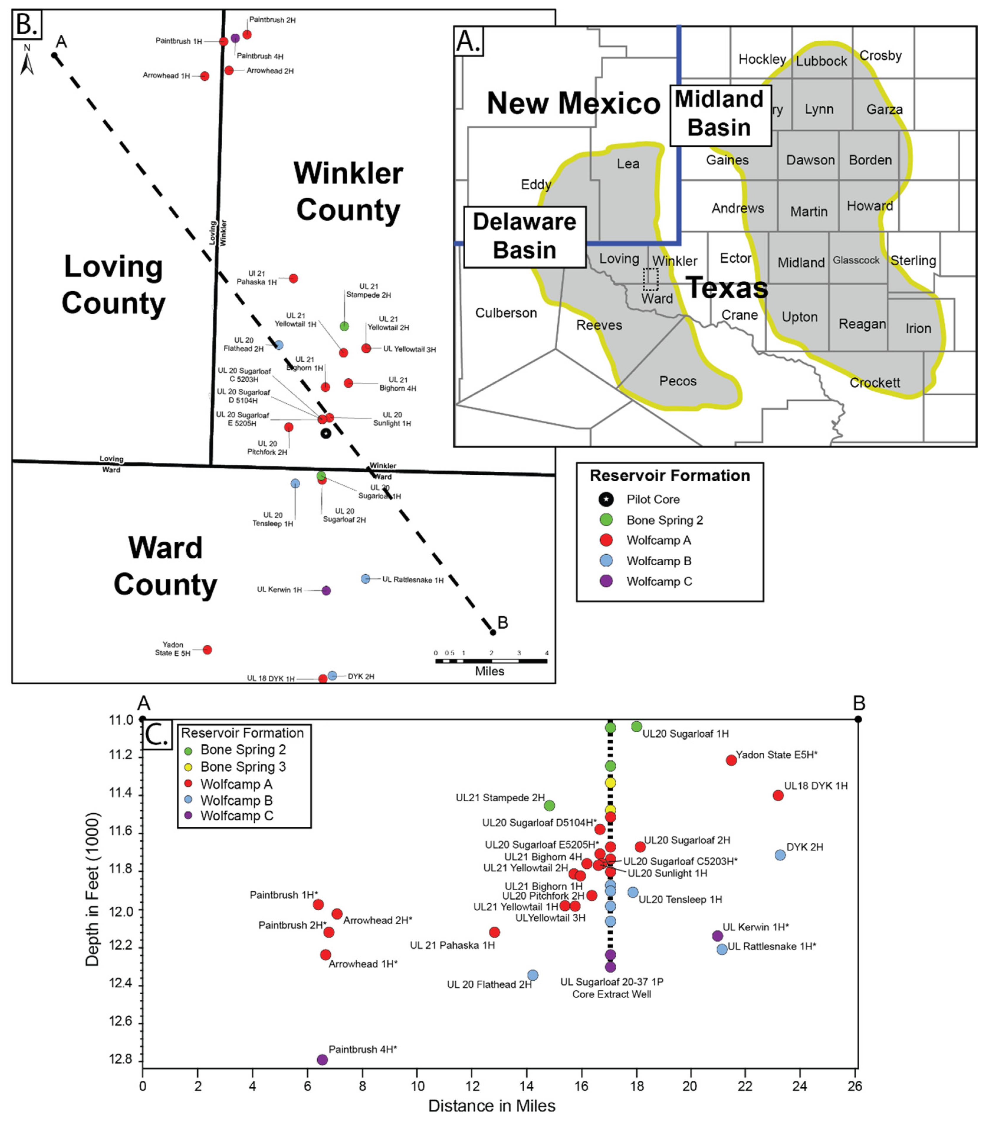
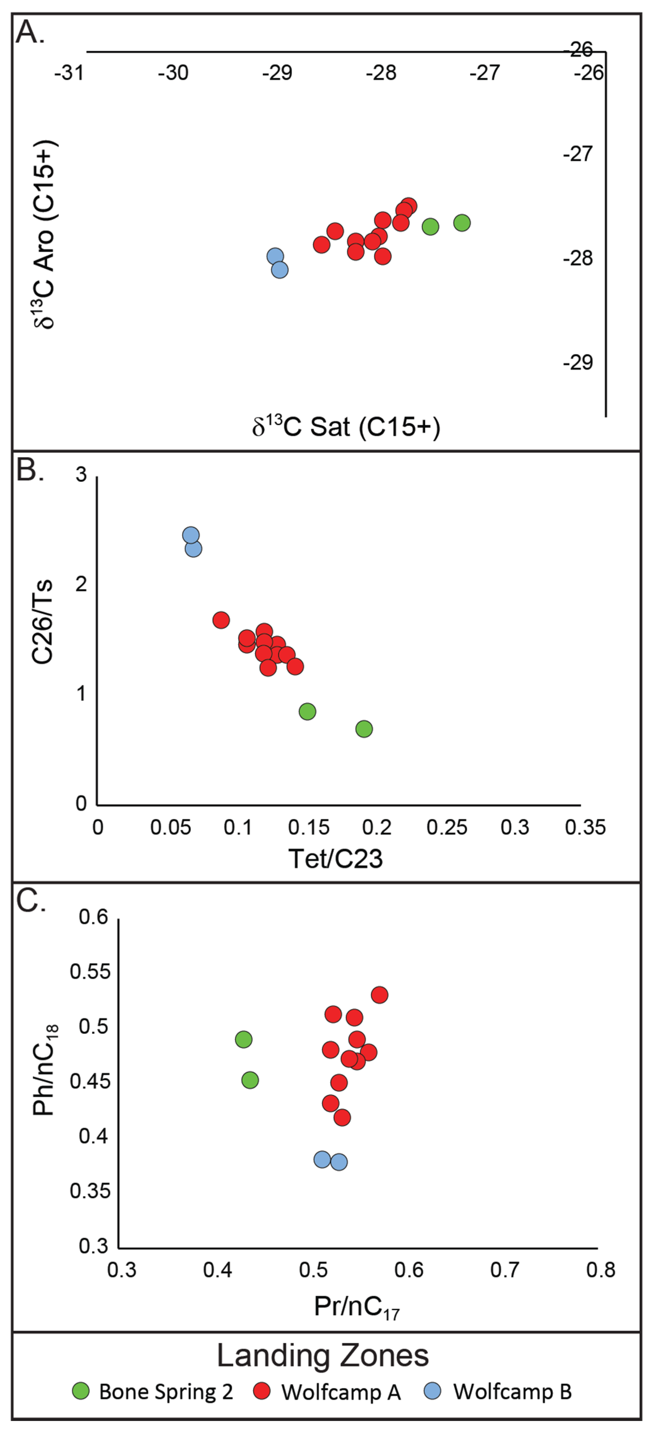
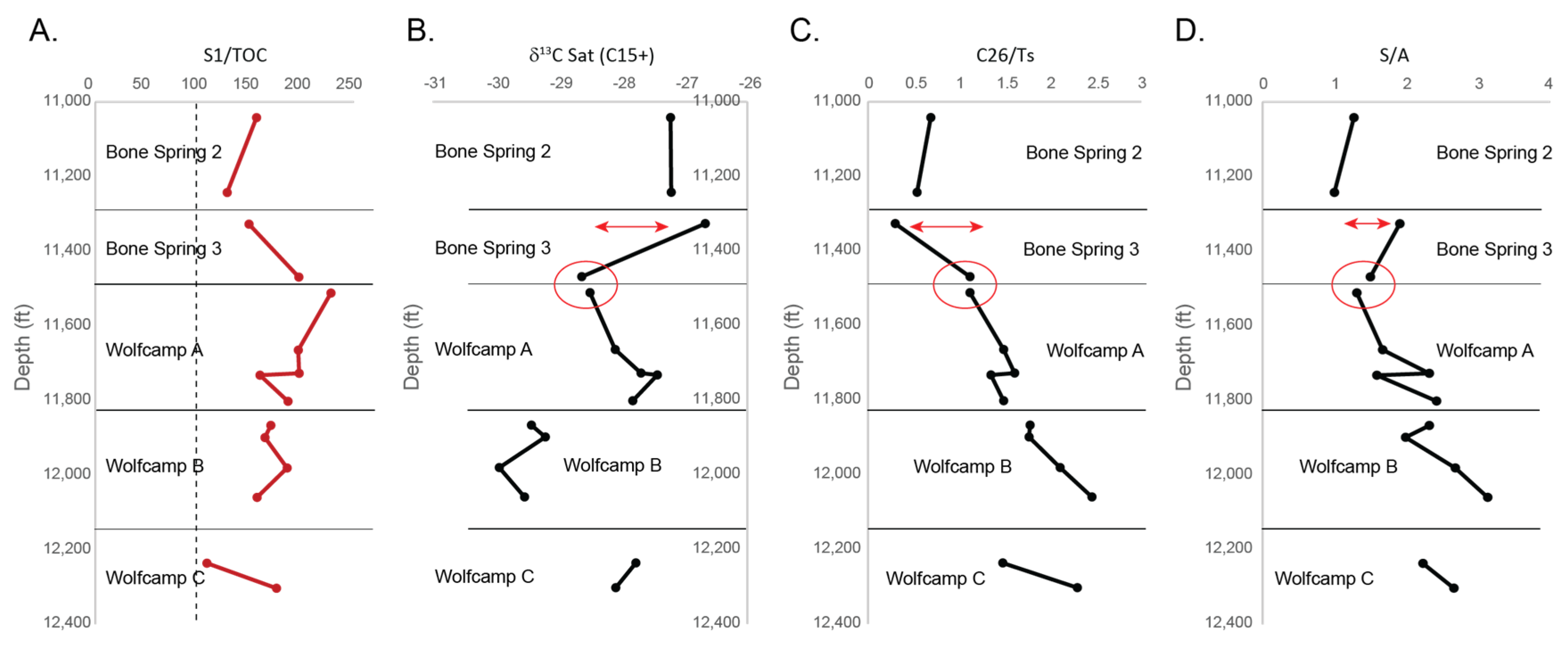
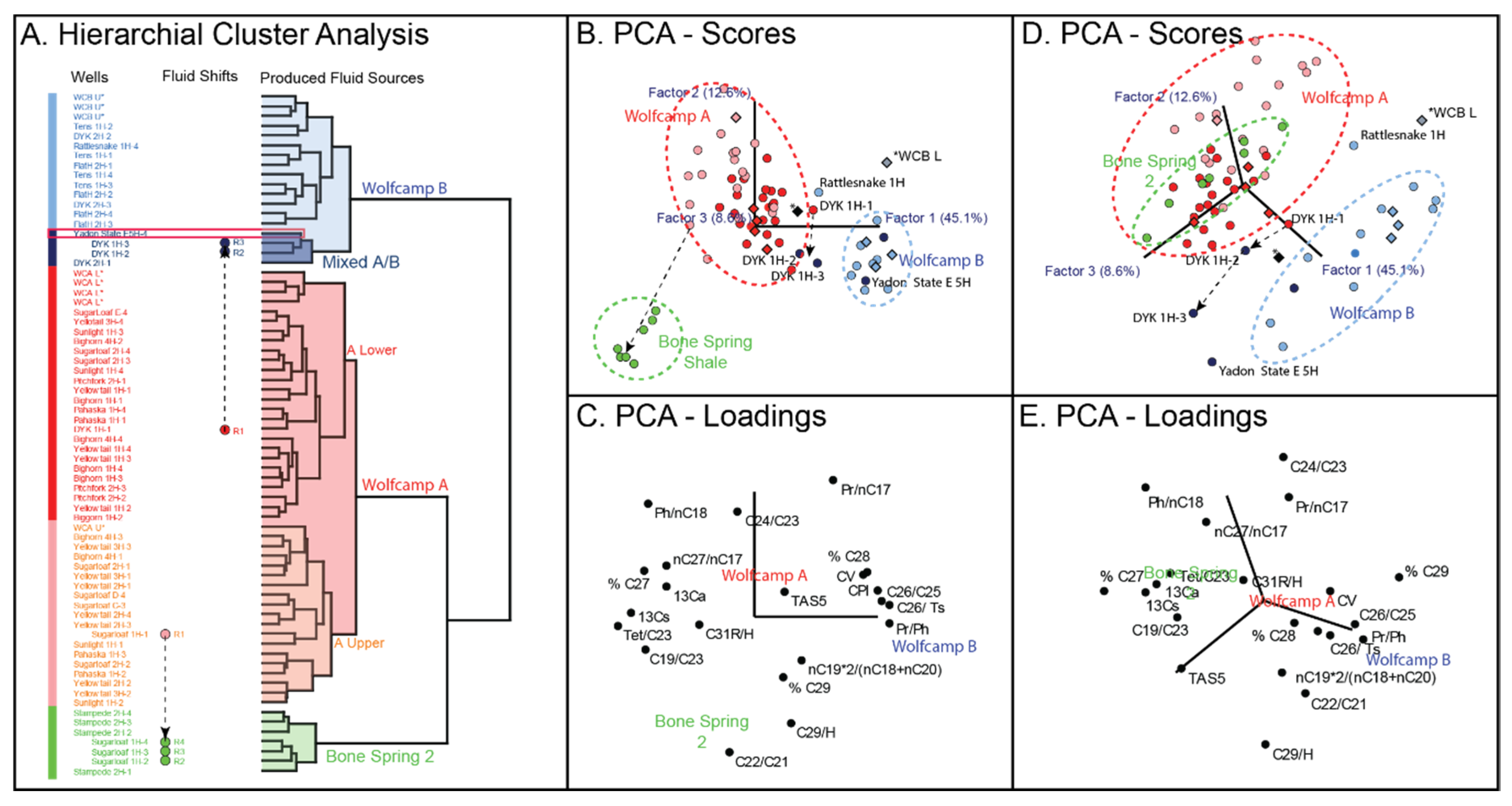
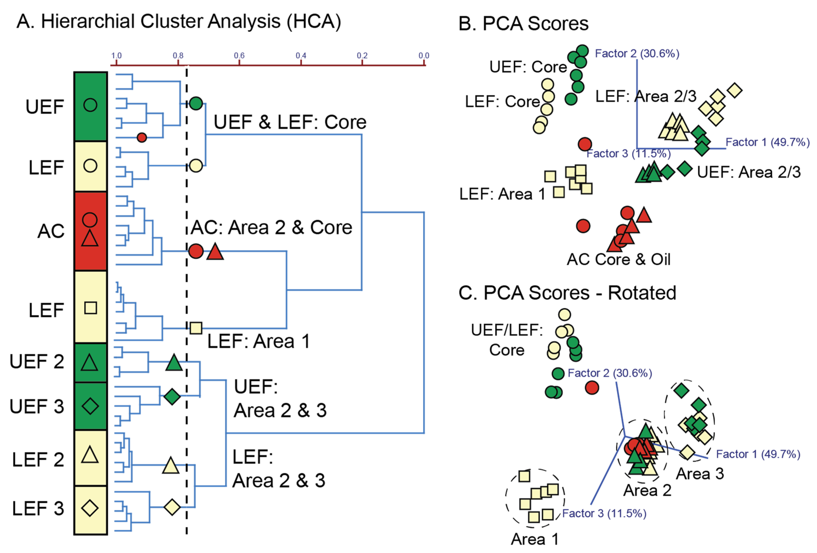
3.2.1. Permian Basin: Core-to-Oil Correlation & Time Lapse Geochemistry

The Permian Basin located in southwest Texas and southeastern New Mexico is the largest unconventional play in the USA. The Delaware Basin, the westerly sub-basin of the Permian, is prodigiously productive and includes numerous Permian age formations with proven hydrocarbon resources (Guadeloupian, Leonardian, and Wolfcampian) as well as the deeper Pennsylvanian/Devonian Formations [31,32]. The case study from the Delaware Basin discussed here has been outlined in considerable detail in previous work [18] and only a summary of the findings and its impact on reservoir geochemistry, specifically extracted fluids to produced oil correlations, will be discussed. This case study uses samples from Winkler, Ward, and Loving Counties in Texas (Figure 4). This project consisted of 4 sampling rounds, a total of 74 produced oils from 26 individual wells, 15 core extracts from a single well in Winkler County and target zones in the Bone Spring 2 (BS 2), Wolfcamp A (WC A), Wolfcamp B (WC B) and Wolfcamp C (WC C) Formations (Figure 4). The initial “baseline” assessment of the fluids in this study focused on 15 wells in the BS 2, WC A and WC B formations, and used no core/cuttings material. Once baseline separation of the fluids was determined, additional wells, sampling rounds and core extract was added to the project to get a better handling on landing zone variation, source correlations and contributions.

Geochemical results from the initial baseline samples revealed that the signature of the produced oils differed based upon the targeted landing formation, i.e., BS 2, WC A and WC B (Figure 5). Given our understanding of the regional geochemical variation in oils across the Permian Basin also based on formation [33], the geochemical differences can be inferred to be predominantly associated with these different landing formations. This evident geochemical compartmentalization appropriately convinced the operator that they were producing distinct fluids from the various target zones, and therefore assessing fluid changes over time and determining fluid ingress and co-mingling was achievable. Three additional fluid rounds were collected (sampling approximately every three months), additional wells producing from the same and new target zones were added and core material was provided from the UL Sugarloaf 20–37 1P pilot well for correlation and allocation purposes (Figure 4). Source rock-to-oil correlation has been a foundational task of petroleum system geochemistry for decades and there is considerable literature on the subject [20,21,22]. Correlation, however, is not the same as allocation. The former is looking to assess geochemical relationships but is not necessarily quantitative, while allocation, on the other hand, by its very definition is a quantitative assessment whereby the core signatures are the de facto end-member fluids of an un-mixed system. In this case study, the purpose of adding core samples was for statistical correlation assessment that would better define what zones were contributing to production, but the extracts were not intend to serve as end-members for allocation work, particularly when produced oils were available for the task.

Hydrocarbons were extracted from 15 sub-samples of the core as illustrated in Figure 6, all of which were TOC and free hydrocarbon rich. The geochemical signature of these core extracts was comparable to that from the baseline oil samples (Figure 5), with the different target formations preserving distinct and similar–albeit not identical–geochemical signatures as those from the produced oils in the same landing formations (Figure 7). However, while the geochemical signatures of the extracts are similar to those of the produced oils, there are differences which can have several explanations:

• The produced oils are all “mixed” fluids producing, to a variable extent, from more than one compartment/end-member.
• The extracted hydrocarbons, by their very nature, are not fully reflective of the produced oils and therefore some offset is expected.
• The extracted hydrocarbons represent a single core plug and while stratigraphic variability can be accounted for, to some extent, lateral variability cannot (Figure 3B). The producing laterals, being several miles in length, are therefore producing from varying organofacies is not reflected in the core fluids.
• “Migration happens”, both inter- and intra-formational (Figure 6), even within tight shales over geological time scales, and this would mean producing wells will not necessarily be geochemically similar to core extracts from nearby wells.

The reasoning for the offset is almost certainly a combination of all of these factors, all of which complicate the idea that extracted core fluids can be used directly for specific quantitative allocation assessments in unconventional plays. Every project is different and the utility of this approach, even where the results look appropriate, may only extend to the scale of a limited number of wells. What this case study highlights very well is that the real value of the extract data is not in allocation, rather it is in the correlation of the produced oils to the extracted hydrocarbons from the same target laterals. This step confirmed the initial SRV potential, giving a solid case from which to estimate the DRV from the produced oils. Using this oil–extract correlation, the following questions can be addressed:

• Where is my oil sourced from (Figure 7)?
• Is there evidence for mixing (Figure 7 and Figure 8)?
• Is the fluid changing through time (Figure 8)?

By expanding the geochemical dataset beyond the 1st round of produced oils, and using the relationships evident from the initial baseline work, all of the above questions can be answered. The BS 2, WC A, and WC B target formations, through time, all retain evident geochemical separation, with the exception of the BS 2 landed Sugarloaf 1H well (Figure 7). This sample looked geochemically similar to the other BS 2 well (Stampede 2H) in the 1st round of sampling (Figure 5). However, with the addition of more samples and timestamps, it is evident that the Sugarloaf 1H well is producing a co-mingled BS 2 and WC A oil in the 1st round of sampling, which by the time the 2nd sampling round took place had transitioned to a dominantly BS 2 producing well, matching up with the landing zone (Figure 7). This produced oil remained consistently BS 2 through all subsequent sampling rounds and was the only sample to show a statistically significant shift through time and evidence for production induced co-mingling (Figure 8). While there was some geochemical changes in other producing wells, none were statistically significant, and this points towards this geochemical variation being indicative of “cleaning up” of the drained rock volume (DRV) with time rather than a change in fluid contributions across target zones. As part of this study, one of the 1st round WC A oils was mixed with one of the WC B oils in the laboratory to highlight how this sample would cluster in PCA space relative to the proposed WC A and WC B source fluids (Figure 8).Two of the wells in the southern section of the study area (Figure 4) consistently grouped with this mixed A/B sample through all sampling rounds (UL 18 DYK 1H and Yadon State E5H). Both of these potentially co-mingled wells are WC A landed and situated in close proximity to a known fracture zone. All of this information, i.e., core extract data, produced oils through time, in-house mixed fluid, and the geologic context, conclude with the hypothesis that the migration of deeper WC B fluids, along fracture pathways, has generated a geologic mix of WC A and B fluids in the reservoir of these wells, and co-mingling in these samples is therefore geologic and not from completions or production.

This case study highlights the considerable value offered by examining the geochemistry of produced oils, particularly in scenarios where core/cuttings are contaminated, unaffordable or inaccessible. The addition of core material adds significant context and can greatly reduce uncertainty, but only if used appropriately to reinforce the evidence from the produced fluids. This case study also shows that geochemistry is only one aspect to be considered. Geologic context, production data, and field development information should all be considered when explaining SRV and DRV distribution and fluid changes within a development area.

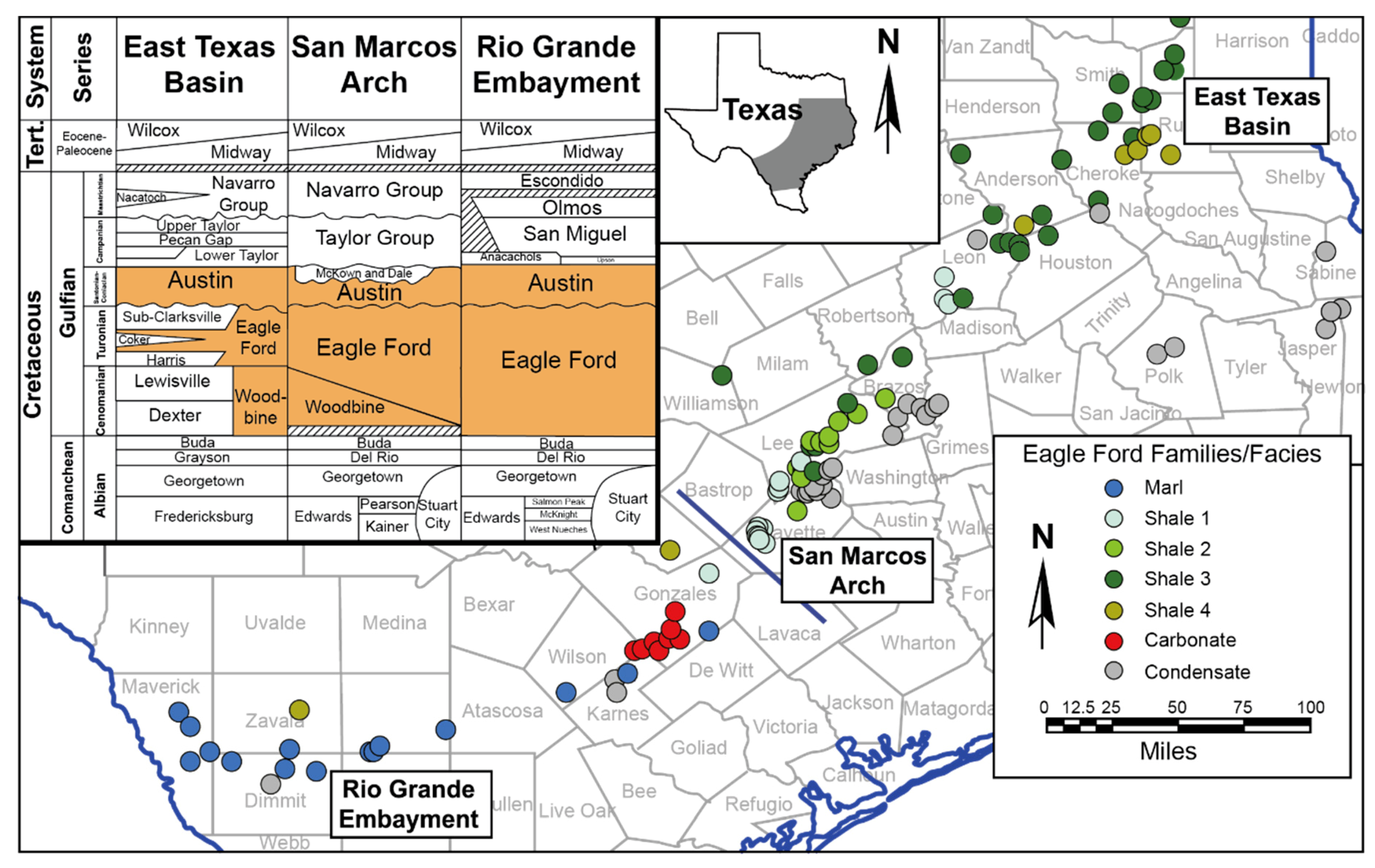
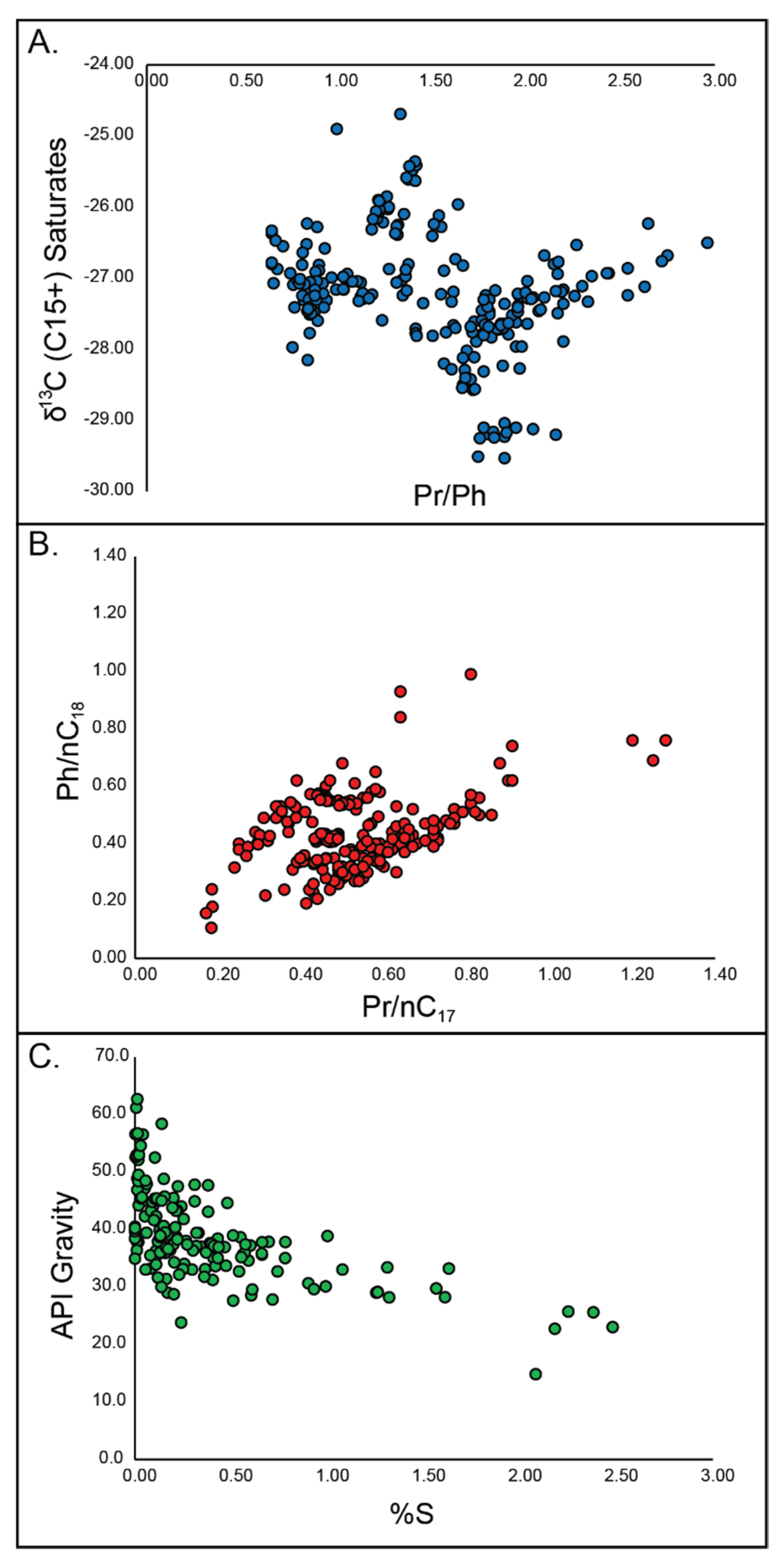
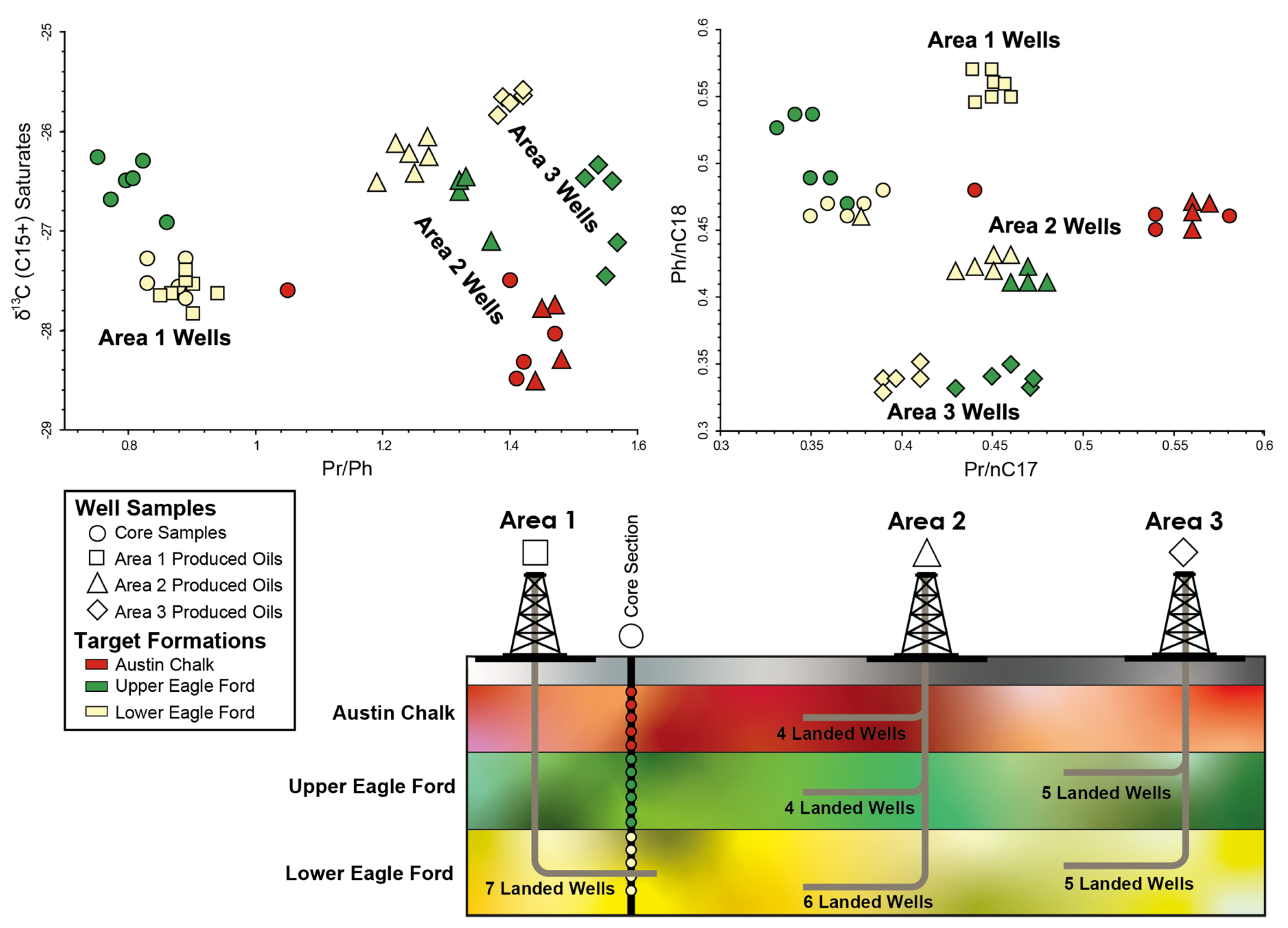
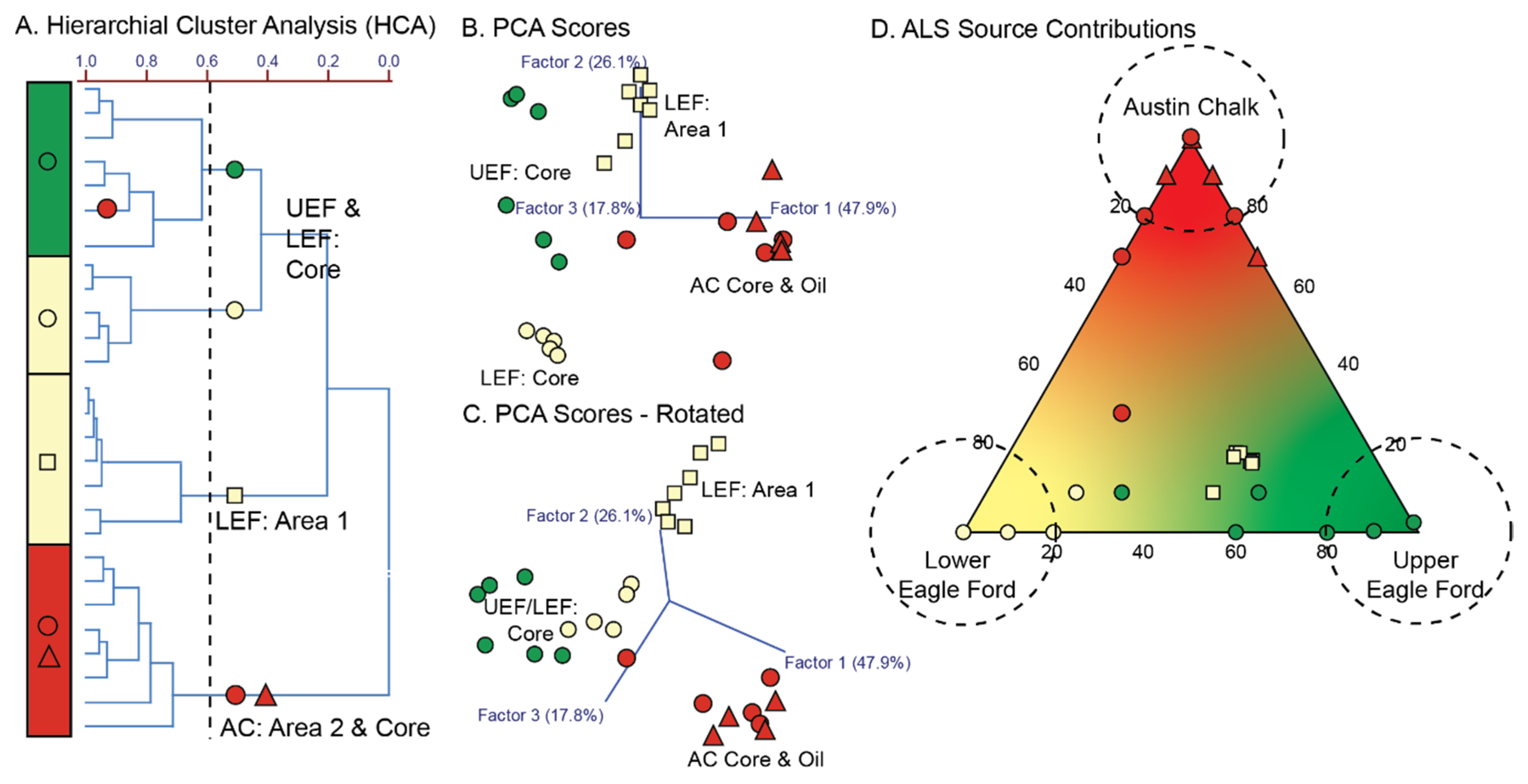
3.2.2. Permian Basin: Eagle Ford Play: Organofacies Variation, Migration & Allocation

One of the primary reasons that using core extracts, as end-members in unconventional systems, was expected to be successful is that many of these plays are primarily self-sourcing. However, “migration happens” [34] and even in these relatively tight lithologies, expulsion and migration do indeed happen, both naturally and from stimulation, otherwise production wouldn’t be possible. The Eagle Ford Shale is a prime example of a play which contains both self-sourced hydrocarbons (Lower Eagle Ford) and dominantly migrated hydrocarbons (Upper Eagle Ford, Austin Chalk and Buda amongst others). The Eagle Ford Play stretches from Southwest Texas to Northeastern Louisiana in the USA (Figure 9) and is one of the most active unconventional systems in the world, producing more than one million barrels of oil/condensate per day through July 2020 [35]. Stratigraphically, the focus for hydrocarbon production in this play is, unsurprisingly, the Cretaceous-aged Eagle Ford shale, although both the underlying Buda Formation and the overlying Austin Chalk are increasingly common target formations for unconventional production (Figure 9). There is a plethora of early literature on the stratigraphy and organic geochemistry of the Eagle Ford [36,37], although this work focused on conventional reservoir systems. In the past few years, the geochemical focus has largely shifted to unconventional fluid production [38], with the work of Jweda et al. [5] leading to a burgeoning interest in the application of reservoir geochemistry and its methodologies in this and other unconventional systems [6,18,25,28].

The Eagle Ford Play represents an interesting challenge from an unconventional reservoir geochemistry stand point. Time lapse geochemistry, as outlined in the previous example, is relatively straightforward and changes across a range of scales (well, pad, regional, etc.) can be readily identified. In this case study, we focus much of the discussion on production allocation and how numerous factors can complicate the data geochemists have to work with:

• Maturity: Many operators are producing higher maturity fluids that lack biomarkers. This is not an insurmountable challenge as there are numerous other technique available which can characterize these samples (HRGC, δ¹³C_VPDB and δ³⁴S_VCDT Isotopes, GC-MSMS QQQ biomarkers, etc.). However, increased maturity does reduce the analytical avenues available, but more importantly, it adds additional complexity where fluids from the same target zone differ in maturity due to lateral depth variations. Therefore, it is difficult to assess if fluids from the same target zones are differing due to co-mingling of differing maturity fluids or is it a maturity variation within a single zone.
• Oil-based mud (OBM): Most drilling in the Eagle Ford relies on the use of OBM. From a geochemical stand point, OBM rules out cuttings being used for anything more than a source rock maturity assessment, due to contamination. This may not affect center cut core samples, but additional care must be taken during sampling and preparation.
• Organofacies variation: The Eagle Ford Shale is well known for considerable organofacies variation both stratigraphically and laterally with carbonaceous and shaley input varying across relatively small distances, reducing confidence in quantitative source contribution determination beyond the pad scale [38].
• Migration or self-sourcing: One of the assumptions often made about unconventional allocation work is that the fluids are self-sourced from the lateral target zones. This is the case in many systems and is at least partly evident in the Eagle Ford. However, most of the fluids produced from both the Upper Eagle Ford and the Austin Chalk Formations are generally considered to be at least partially sourced from the Lower Eagle Ford and have migrated into place over geologic time. Therefore, caution must be taken when assuming an evidently co-mingled fluid signature in these formations is evidence of production induced, as it may very well be geologic. Core material can assist with this determination but, given all of the factors noted above, this approach may be limited in scope.

These complications make allocation assignment generally complex. However, this does not mean that discrete fluid compartments can’t be defined or that fluid changes related to production can’t be examined. Those are readily obtainable objectives and provide excellent insight into the dynamics of an operator’s acreage. There can be confusion as to whether a migrated fluid showing a distinct trend with depth can be considered a distinct fluid compartment. Just as with a fully self-sourced production unit, depending upon how that might be defined, any production related co-mingling, as a result of interaction between separate DRV networks is identifiable through the geochemical signature of the oil. Scale, of course, is always important, and the variable geochemical signature of the Eagle Ford is one of the clearest examples of scale. The organofacies of the Eagle Ford-sourced fluids in the southwest (Rio Grande Embayment) are more marly or carbonaceous in character, differing geographically (Figure 9). As you move towards the San Marcos Arch and the East Texas Basin, the Eagle Ford-sourced oils are increasingly shaley in character but statistically break up into at least five distinct oil families [38] (Figure 9). When comparing some of the geochemical variables from these Upper Cretaceous sourced oils (Figure 10), it is striking how significant the potential ranges are. While much of this variation is tied to changes in organofacies, there is also an element of thermal maturity variation and geologic co-mingling. The regional dataset very elegantly highlights how variable fluids sourced, largely, from a single source can be.

However, reservoir geochemistry studies of unconventional systems are rarely designed at such a scale. Most are focused on understanding changes and contributions across individual pads and potentially across multiple pads within a specific, much more localized region (Figure 11). In the example shown in Figure 11, pulled from GeoMark’s proprietary data in Southwest Texas (Figure 9), there are three target production zones (Austin Chalk, Upper Eagle Ford, and Lower Eagle Ford) across three production areas, all of which are within a 10-mile radius of one another. In addition to the wells landed across the target formations in the three areas, there is also core material—and, therefore, geochemical extraction—from a pilot well in close proximity to Area 1. Initial bivariate cross-plots on a selection of the geochemical results (Figure 11) reveal that there are two distinct controls on the geochemical signatures: (1) target formation and (2) geographic location. The most evident control, at least from the data shown, is related to geographic location, which can be considered a proxy for lateral organofacies variation, a point already made throughout this paper. However, it also clear that geochemically there is an obvious distinction in the oils being produced from the Austin Chalk, Upper Eagle Ford, and Lower Eagle Ford formations, and, indeed, in this dataset an obvious consistent lateral trend in the data. Focusing on the individual production areas it is clear that there is a difference in the fluids being produced, which almost certainly ties back to the different zones.

We can test this association theory, at least partly for Area 1, because we have core extracts and the geochemical story from these samples is one of mixed success (Figure 11 and Figure 12). Firstly, as with the produced oils, there are distinct differences in the geochemical signatures of the samples from the Austin Chalk (AC), Upper Eagle Ford (UEF), and Lower Eagle Ford (LEF) target zones. The LEF extracts do match with the LEF produced oils in Area 1, but not across the board geochemically, with some parameters overlapping while others show a clear offset. The LEF produced oils from Areas 2 and 3, which are laterally more disparate, show no overlap whatsoever with the LEF core samples, unsurprising given the organofacies variation evident in the Eagle Ford (Figure 9) and the problems of lateral heterogeneity as discussed earlier (Figure 3). However, why do the LEF oils from Area 1 not match with the core extracts perfectly, if the assumption is that this is indeed the source of these fluids? The answer is ultimately three fold:

• Methodologies for extracting fluids—no matter the protocols—do not mimic geologic expulsion and therefore the geochemical signature of the extracted hydrocarbons should not be anticipated to mimic the produced fluids.
• Not all oil properties behave in the same manner. Some properties change very quickly and readily over relatively small migration distances and, therefore, even close proximity to the core extract material is no guarantee of fluid matching.
• The production well is likely producing a fluid which is a combination of a much larger lateral and stratigraphic area than is recorded in the few core extracts from the single comparative well. It should therefore never be expected to be identical—similar? Yes—but with some variability and offset anticipated.

Therefore, while we can quite readily say we see a correlation between the Area 1 LEF oils and the extracted hydrocarbons, allocation presents some problems. There are no UEF produced oils in Area 1 but, even if there were, correlation to those produced oils seem unlikely. All of the UEF produced oils in the other production areas (Figure 11) are offset from the LEF fluids in a consistent direction while the core extracted UEF fluids follow the opposite trend and are much harder to distinguish from the LEF extracted hydrocarbons. It may be that these UEF extracts are simply not comparable to the UEF produced oils across these production areas, or it may indicate something about the UEF production in the other areas themselves. This is where the issue of trying to apply a single core well dataset to a larger area becomes highly subjective. There are no AC produced oils in Area 1 but, interestingly, the AC produced oils from Area 2 correlate closely with these AC extract samples and unlike the LEF correlation, it is consistent across the geochemical data collected (Figure 11). The AC produced oils are almost certainly migrated LEF oils and the extracted hydrocarbons themselves will be from the same source. In this scenario, the AC oils are behaving more as they would in a conventional system where migration and reservoir horizons play a role (in this case, the AC is the reservoir for the migrated LEF oils). This means correlation—and potentially allocation—preserves a much tighter geochemical relationship. One AC extract sample stands out as distinctly different geochemically (Figure 11 and Figure 12). This is the deepest sample stratigraphically and is likely more akin to what would be an UEF migrated fluid.

If we compare all of the production areas and the core samples statistically, the same relationships and clustering, as evident from the bivariate plots, is solidified (Figure 12). Hierarchical Cluster Analysis (HCA) indicates, with the exception of the AC core and oils, the core extracts are distinctly different geochemically from the produced oils across all areas assessed. The LEF produced oils from Area 1 share the greatest similarity to this core, but, they are still offset and statistically form their own group of oils. Although the principal component analysis (PCA) plots indicate a strong correlation between geochemical signature and production Area (Figure 12B,C) the HCA dendrogram suggests statistically the UEF and LEF zones from Areas 2 and 3 are actually closer in similarity to one another than the geographic/lateral control. As indicated in Figure 11, both the HCA and PCA statistics indicate that the AC extracts and oils correlate well with one another, with a single statistical outlier, as evident in previous plots, looking more like an UEF fluid.

Given all of these data, a question arises. Can we effectively allocate any of the produced oil samples back to the core extracts? The results indicate that the LEF and UEF oils from Areas 2 and 3 are too different from the core samples to have any chance of success. However, the Area 1 LEF oils show some similarity and the Area 2 AC oils are an even stronger candidate for allocation. Therefore, we can rerun the HCA and PCA statistics just on the core samples and the Area 1 LEF and the Area 2 AC oils to see what emerges (Figure 13). The correlations and offsets in the HCA and PCA graphs closely mirror those from the larger dataset in Figure 12. Again, as with the earlier figures, the LEF produced oils from Area 1 are closest in similarity to the LEF core extracts, but they are not a direct match. Bearing this in mind we can run the alternating least squares (ALS) algorithm on this dataset and see where the contributions fall out (Figure 13D). Unlike the previous example of ALS allocation discussed (Figure 2), this time, the algorithm was run in active mode, whereby we assigned specific core extracts as the three end-members to allocate to (Austin Chalk, Upper Eagle Ford and Lower Eagle Ford). These were determined by running the ALS algorithm on the core extracts on their own, determining the most geochemically unique samples from each zone and then building an ALS model around these three end-members. The remaining core samples and produced oils then had their source contributions predicted against these end-members. The predicted source contributions do not differ greatly from the qualitative assessment made from the HCA and PCA graphs (Figure 13D).

The AC produced oils allocate closely with the AC end-member extract. The cloud of uncertainty has been suggested at around 20% for these end-members, but given the contribution range on the AC extracts themselves, it may be closer to 30%. The LEF extracts show a similar error at around 20–25% but, from an allocation stand point, none of the Area 1 produced oils correlate with this end-member. It has been clearly shown that the oils are indeed from the LEF, but the precision required for true allocation is not present in this sample set. The UEF end-member is by far the most suspect with the non-end-member defined extracts from this formation trending off towards the LEF source. That is not to say these are incorrect. Given all of the earlier data (Figure 11 and Figure 12), it is entirely expected, and the ternary diagram is reflecting the variability in the geochemistry of these samples. The LEF produced oils from the Area 1 plot at around 60% UEF sourced, 20% LEF and 20% AC and form a relatively tight cluster of source contributions (Figure 13D). This would imply quite a different co-mingling and source scenario than is known from the geochemical data and overall context of these samples. In this case, if an operator had solely relied on the algorithm to report a contribution, the results would be disappointing. Fortunately, context and stronger geochemical correlation tools can also be employed to more readily answer these questions. This result highlights that while allocation can and does work, it is not a given and even a close proximity to your core extract samples is not a guarantee of success. Indeed, focusing purely on source contributions, as opposed to defining a geochemical framework and associated relationships, may result in wrong answers and incorrect interpretation.

3.3. Best Practices for Designing a Successful Reservoir Geochemistry Project

The case studies discussed in this paper emphasize the value of produced oil in reservoir geochemistry work and how core material can be useful, where available, but is not a necessity. These case studies also demonstrate how unconventional reservoir geochemistry is used to address key fluid character questions for operators in a production setting:

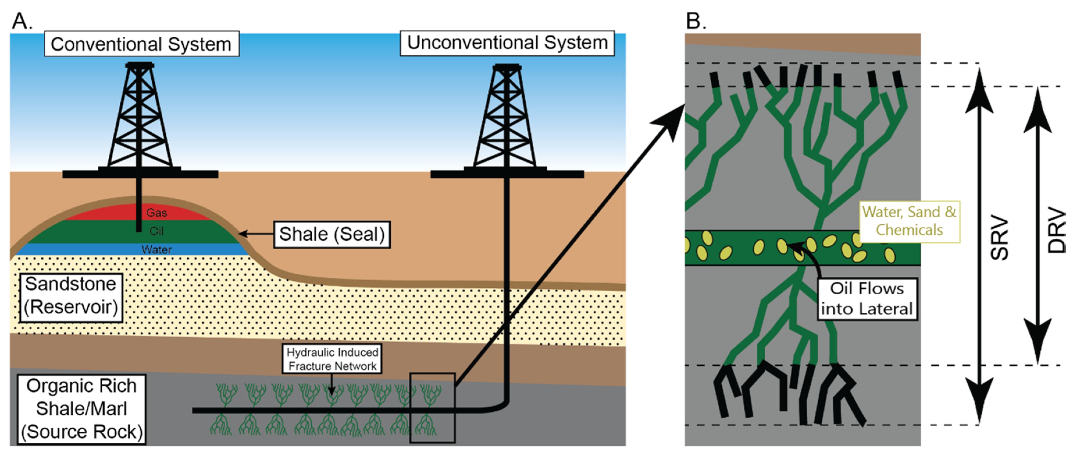
• Where is my oil draining from (DRV)?
• How much oil should be available (SRV)?

Both questions are linked and use similar data to obtain an answer. An efficient plan is needed to collect data, primarily from produced oils, and then appropriate analysis in conjunction with other geologic and production data will yield the best results. A statistical approach is recommended for unconventional production because it can use a wide range of geochemical data, while providing a robust assessment of fluid production across multiple discrete fluid compartments, and identify significant shifts in production sources while avoiding noise generated from natural variability. Extracts from core samples can provide useful information of downhole fluid relationships but the produced oils themselves are what these studies should predominantly focus upon because they offer direct information on the production and connectivity dynamics within a development program. Allocation contributions have their place and can provide valuable descriptions of production contributions. However, they are reflective of a very specific, and relatively restrictive, set of assumptions and geochemical data. Understanding the “cloud of uncertainty” associated with this quantification, as well as the geographic and stratigraphic limitations, will ensure maximum value when utilizing these data.

With all of these considerations and caveats borne in mind we would suggest a number of best practice considerations when designing and undertaking a reservoir geochemistry study in unconventional systems:

• Start with the produced oils: This is the easiest and most cost-effective way to build an initial understanding of what is being produced and from where. The initial geochemical results from this sample set, and potential evident compartmentalization, will dictate the future direction of the program.
• Sample more, analyze less: Collecting fluid (and gas) samples from the separator is relatively quick and low cost and can then go into storage for later use. It’s not necessary to analyze all of the collected samples, but having them available when changes in the geochemistry are identified can help determine the cause and specific timescale of the variation, and therefore, the correct response.
• Good data starts in the field: If you want to maximize your data return then sample integrity is crucial and sample collection procedures need to be both robust and consistent with appropriate labelling. This seems like a small point but, it can be crucial to both the success of the project and the viability of the data interpretation.
• More is better than less: Time lapse geochemistry can be carried out on a single well and comparison to existing datasets can provide significant insight into source and mixing. However, larger sampling sets provide much better understanding on source variability across an operator’s acreage and ensures much more robust statistical comparisons.
• Extracted hydrocarbons from core are important but not the crux of these projects: Core material provides valuable data, and tangible evidence, rather than inference on the source of the produced oils. However, this material is limited in range. Furthermore, given the nature of unconventional systems, the source of the fluids being targeted is generally well known, and therefore correlations are merely confirming those suspicions and identifying outliers where geologic context might be playing a role.
• Source contributions can be assigned but quantification may not add value: There are numerous mathematical algorithms and software programs available to un-mix oils and assign source contributions. However, these programs do not solve the hardest part of the problem, namely determining the ‘end-members’. As was discussed here, defining a representative end-member of a dynamic and varying system will produce wide errors on quantified allocations. There are a number of ways to get to ‘an’ answer for allocation, all of which contain a nugget of truth, but all assume a level of homogeneity and consistency which is not the norm in unconventional systems.
• Continue sampling even when fluid production remains stable: Although the majority of changes in fluid production are reported during the earliest stages of well production, changes in more established wells can and do occur. These changes are most often related to field developments, such as the addition of new wells and shut-ins, which can lead to changes in the DRV of existing wells. As said above, sample more, analyze less, so that the samples are available for analysis when needed.

The last point to consider is to directly address the overemphasis that has been placed on using extracts from core or cuttings material for use in source allocation studies. Core is often a limiting factor and, therefore, cuttings have been suggested as a cheaper and more readily available alternative [6]. However, as useful as cuttings may be in identifying source zones and so forth, their provenance is much more difficult to confirm than core material, a crucial tenant when it comes to robust allocation work. Oil-based mud (OBM) is a common contaminant and light hydrocarbon loss (LHC) is the norm, even more so than in core, no matter how the sample material is collected and stored [17,18,19]. The usage of cuttings, while cheaper and easier to collect, does not remove the issues raised when using core samples, but merely provides an additional set of problems to deal with rather than improving understanding of the specific allocation contributions of produced fluids. That is not to say that detailed geochemical core data is not useful, as its value has been demonstrated in this paper, but only if it is used in the appropriate manner. Oil–core correlations and the statistical assessment of these data provides valuable information about the source of fluids. However, like-for-like comparison, an appropriate scale (well-to-well), and an appreciation of the uncertainties, particularly pertinent to unconventional systems, are essential. If allocation is considered absolutely essential, then end member comparison should be made between produced fluids (like-for-like), not between core extract fluids and produced fluids, as they are not interchangeable.

4. Conclusions

The examples and discussion presented in this paper highlight the importance of reservoir geochemistry studies in unconventional plays. However, this paper makes clear that reservoir geochemistry must be well designed and appropriately applied. The resulting data can be of immeasurable value and ensure the right decisions are made to maximize production across an operator’s acreage. The dynamic and heterogenic nature of unconventional systems is best handled through a statistical approach that can balance the natural variance and provide direct guidance for an operator’s development program. While every project will be developed and adapted individually based upon the operator’s objectives, geochemistry is an important tool to understand DRV and variations/changes in production data and will ensure maximum ROI for any project.

References

1. Ajisafe, F.; Solovyeva, I.; Morales, A.; Ejofodomi, E.; Marongiu Porcu, M. Impact of well spacing and interference on production performance in unconventional reservoirs, Permian Basin. In Proceedings of the Unconventional Resources Technology Conference, Austin, TX, USA, 24–26 July 2017. [Google Scholar] [CrossRef]
2. Malayalam, A.; Bhokare, A.; Plemons, P.; Sebastian, H.; Abacioglu, Y. Multi-disciplinary integration for lateral length, staging and well spacing optimization in unconventional reservoirs. In Proceedings of the Unconventional Resources Technology Conference, Denver, CO, USA, 25–27 August 2014. [Google Scholar] [CrossRef]
3. Zeynal, A.R.; Kashikar, S. Understanding and quantifying variable drainage volume for unconventional wells. In Proceedings of the Unconventional Resources Technology Conference, San Antonio, TX, USA, 1–3 August 2016. [Google Scholar] [CrossRef]
4. Yong, Y.K.; Maulianda, B.; Wee, S.C.; Mohshim, D.; Elraies, K.A.; Wong, R.C.K.; Gates, I.D.; Eaton, D. Determination of stimulated reservoir volume and anisotropic permeability using analytical modelling of microseismic and hydraulic fracturing parameters. J. Nat. Gas Sci. Eng. 2018, 58, 234–240. [Google Scholar] [CrossRef]
5. Jweda, J.; Michael, E.; Jokanola, O.; Hofer, R.; Parisi, V. Optimizing field development strategy using time-lapse geochemistry and production allocation in Eagle Ford. In Proceedings of the Unconventional Resources Technology Conference, Austin, TX, USA, 24–26 July 2017. [Google Scholar] [CrossRef]
6. Liu, F.; Wu, J.; Jin, M.; Hardman, D.L.; Cannon, D. From reservoir characterization to reservoir monitoring: An integrated workflow to optimize field development using geochemical fingerprinting technology. In Proceedings of the Unconventional Resources Technology Conference, Austin, TX, USA, 20–22 July 2020. [Google Scholar] [CrossRef]
7. Yang, W.; Casey, J.F.; Gao, Y.; Li, J. A new method of geochemical allocation and monitoring of commingled crude oil production using trace and ultra-trace multi-element analyses. Fuel 2019, 241, 347–359. [Google Scholar] [CrossRef]
8. Bennett, B.; Adams, J.J.; Larter, S.R. Oil fingerprinting for production allocation: Exploiting the natural variations in fluid properties encountered in heavy oil and oil sand reservoirs. In Proceedings of the Frontiers + Innovation—CSPG CSEG CWLS Convention, Calgary, AB, Canada, 4–8 May 2009; pp. 157–160. [Google Scholar]
9. Kaufman, R.L.; Ahmed, A.S.; Elsinger, R.J. Gas chromatography as a development and production tool for fingerprinting oils from individual reservoirs: Applications in the Gulf of Mexico. In Proceedings of the 9th Annual Research Conference of the Society of Economic Paleontologists and Mineralogists, New Orleans, LA, USA; Schumaker, D., Perkins, F.B., Eds.; GCSSEPM Foundation: Houston, TX, USA, 1990; pp. 263–282. [Google Scholar]
10. Kaufman, R.L.; Ahmed, A.S.; Hempkins, W.B. A new technique for the analysis of co-mingled oils and its application to production allocation calculations. In Proceedings of the 16th Annual Indonesian Petroleum Association Convention, Jakarta, Indonesia, 20–22 October 1987; pp. 247–268. [Google Scholar]
11. Lareau, H.; Dahl, J.; Clark, A.; Parney, B.; Friedman, S. Utilizing geochemical analysis in unconventional reservoirs to allocate produced oils to Stratigraphic zone. In Proceedings of the International Conference and Exhibition, Barcelona, Spain, 3–6 April 2016. [Google Scholar] [CrossRef]
12. McCaffrey, M.A.; Baskin, D.K.; Patterson, B.A. Geochemical allocation of commingled oil production and/or commingled gas production from 2–6 Pay zones. In Proceedings of the AAPG Hedberg Conference ‘Applications of Reservoir Fluid Geochemistry’, Vail, CO, USA, 8–11 June 2010. [Google Scholar]
13. McCaffery, M.A.; Baskin, D.K. Applying oil fingerprinting to unconventional reservoirs in the permian basin for characterization of frac height and quantification of the contribution of multiple formations to commingled production. In Proceedings of the Unconventional Resources Technology Conference, San Antonio, TX, USA, 1–3 August 2016. [Google Scholar] [CrossRef]
14. Hwang, R.J.; Baskin, D.K.; Teerman, S.C. Allocation of commingled pipeline oils to field production. Org. Geochem. 2000, 31, 1463–1474. [Google Scholar] [CrossRef]
15. Peters, K.E.; Ramos, L.S.; Zumberge, J.E.; Valin, Z.C.; Bird, K.J. De-convoluting mixed crude oil in Prudhoe Bay Field, North Slope, Alaska. Org. Geochem. 2008, 39, 623–645. [Google Scholar] [CrossRef]
16. Kornacki, A.S.; Westrich, J.T. Applying HC fingerprinting technology to determine the amount of oil produced from hydraulically-fractured wolfcamp reservoirs using petroleum samples extracted from conventional core plugs. In Proceedings of the Unconventional Resources Technology Conference, Austin, TX, USA, 24–26 July 2017. [Google Scholar] [CrossRef]
17. Barrie, C.D.; Donohue, C.M.; Zumberge, J.A.; Rocher, D.; Jarvie, B.; Taylor, K.W.R. Emerging techniques and methods for improving core-to-oil and oil-zone production correlations in reservoir geochemistry. In Proceedings of the Conference Proceedings 29th International Meeting on Organic Geochemistry, Gothenburg, Sweden, 1–6 September 2019. [Google Scholar] [CrossRef]
18. Barrie, C.D.; Donohue, C.M.; Zumberge, J.A. A statistical approach to understanding fluid geochemistry changes in unconventional plays. In Proceedings of the Unconventional Resources Technology Conference, Austin, TX, USA, 20–22 July 2020. [Google Scholar] [CrossRef]
19. Donohue, C.M.; Barrie, C.D.; Jarvie, B.; Zumberge, J.A.; Zumberge, J. A comparison of hydrocarbon extraction techniques: Trying to make a mountain from a mole hill. In Proceedings of the Unconventional Resources Technology Conference, Austin, TX, USA, 20–22 July 2020. [Google Scholar] [CrossRef]
20. Zumberge, J.E. Prediction of source rock characteristics based on terpane biomarkers in crude oils: A multivariate statistical approach. Geochim. Cosmochim. Acta 1987, 51, 1625–1637. [Google Scholar] [CrossRef]
21. Telnaes, N.; Cooper, B.S. Oil-source rock correlation using biological markers, Norwegian continental shelf. Mar. Pet. Geol. 1991, 8, 425–432. [Google Scholar] [CrossRef]
22. Wang, Y.-P.; Zou, Y.-R.; Shi, J.-T.; Shi, J. Review of the chemometrics application in oil-oil and oil-source rock correlations. J. Nat. Gas Sci. 2018, 3, 217–232. [Google Scholar] [CrossRef]
23. Whitson, C.H.; Alqahtani, F.M.; Chuparova, E. Fluid heterogeneity on a well-box scale in tight unconventional reservoirs. In Proceedings of the Unconventional Resources Technology Conference, Houston, TX, USA, 23–25 July 2018. [Google Scholar] [CrossRef]
24. Yurchenko, I.A.; Moldowan, J.M.; Peters, K.E.; Magoon, L.B.; Graham, S.A. Source rock heterogeneity and migrated hydrocarbons in the Triassic Shublik Formation and their implication for unconventional resource evaluation in Arctic Alaska. Mar. Pet. Geol. 2018, 92, 932–952. [Google Scholar] [CrossRef]
25. Long, H.; Michael, E.; Bordoloi, S.; Liu, Y.; Rajappa, B.; Weaver, B.; McMahan, N.; McLin, K. Integrating oil and water geochemistry to assess SRV and DRV in the bakken/three forks hybrid play. In Proceedings of the Unconventional Resources Technology Conference, Austin, TX, USA, 20–22 July 2020. [Google Scholar] [CrossRef]
26. Liu, F.; Michael, E.; Johansen, K.; Brown, D.; Allwardt, J. Time-lapse geochemistry (TLG) application in unconventional reservoir development. In Proceedings of the Unconventional Resources Technology Conference, Austin, TX, USA, 24–26 July 2017. [Google Scholar] [CrossRef]
27. Zumberge, J.E.; Russell, J.A.; Reed, S.A. Charging of Ellis Hills reservoirs as determine by oil geochemistry. AAPG Bull. 2005, 89, 1347–1371. [Google Scholar] [CrossRef]
28. Kornacki, A.S.; Baskin, D.K.; McCaffery, M.A. Using statistical techniques to identify end members for allocating commingled oil samples produced from unconventional reservoirs. In Proceedings of the AAPG Annual Convention and Exhibition, Salt Lake City, UT, USA, 20–23 May 2018. [Google Scholar]
29. Zhan, Z.-W.; Zou, Y.-R.; Shi, J.-T.; Sun, J.-N.; Peng, P. Unmixing of mixed oil using chemometrics. Org. Geochem. 2016, 92, 1–15. [Google Scholar] [CrossRef]
30. Peters, K.E.; Walters, C.C.; Moldowan, J.M. The Biomarker Guide, 2nd ed.; Cambridge University Press: Cambridge, UK, 2005; pp. 608–640. [Google Scholar]
31. Jarvie, D.M.; Prose, D.; Jarvie, B.M.; Drozd, R.; Maende, A. Conventional and unconventional petroleum systems of the delaware basin. In Proceedings of the AAPG Annual Convention and Exhibition, Houston, TX, USA, 2–5 April 2017. Search and Discovery Article 10949. [Google Scholar]
32. Alimahomed, F.; Malpani, R.; Jose, R.; Defeu, C.; Ignacio Velez, A.; Haddad, E. Development of the stacked play in the delaware basin. In Proceedings of the Unconventional Resources Technology Conference, Houston, TX, USA, 23–25 July 2018. [Google Scholar] [CrossRef]
33. Curtis, J.C.; Zumberge, J.E. Permian basin petroleum systems—Geochemical insight into hydrocarbon generation, migration and well performance. In Proceedings of the Unconventional Resources Technology Conference, Houston, TX, USA, 23–25 July 2018. [Google Scholar] [CrossRef]
34. Zumberge, J.E.; Curtis, J.B.; Reed, J.D.; Sonnenfield, M.D. Migration happens: Geochemical evidence for movement of hydrocarbons in unconventional petroleum systems. In Proceedings of the Unconventional Resources Technology Conference, San Antonio, TX, USA, 1–3 August 2016. [Google Scholar] [CrossRef]
35. Texas Railroad Commission. Available online: https://www.rrc.state.tx.us/oil-gas/major-oil-and-gas-formations/eagle-ford-shale-information (accessed on 30 September 2020).
36. Liro, L.M.; Dawson, W.C.; Katz, B.J.; Robison, V.D. Sequence stratigraphic elements and geochemical variability within a “Condensed Section”: Eagle Ford Group, East-Central Texas. Gulf Coast Assoc. Geol. Soc. Trans. 1994, 44, 393–402. [Google Scholar]
37. Dawson, W.C. Limestone microfacies and sequence stratigraphy: Eagle Ford Group (Cenomanian-Turonian) North-Central Texas Outcrops. Gulf Coast Assoc. Geol. Soc. Trans. 1997, 47, 99–105. [Google Scholar]
38. Zumberge, J.E.; Illich, H.; Waite, L. Petroleum geochemistry of the cenomanian–turonian eagle ford oils of South Texas. In The Eagle Ford Shale: A Renaissance in U.S. Oil Production; Breyer, J.A., Ed.; American Association of Petroleum Geologists: Houston, TX, USA, 2016; Volume 110, pp. 135–165. [Google Scholar]
Figure 1. (A). Schematic illustration of the difference between “conventional” and “unconventional” petroleum systems and the target formations for production. (B). Illustration of the difference between the “Stimulated Rock Volume” (SRV) and the “Drained Rock Volume” (DRV) in an unconventional production formation.
Minerals 10 01105 g001
Figure 2. Source Contribution results for artificially mixed samples in the laboratory. The top three graphs are the individual oil samples and their known contributions (blue) compared with the calculated contributions from compositional data (red). The bottom three graphs are the same individual oil sample contributions comparing known contributions (blue) to the calculated contributions from ratio data (green). The curvature and offset in the ratio data is evident across all three contributing samples. The full comparative results are shown in Table 1.
Minerals 10 01105 g002
Figure 3. Schematic diagrams to illustrate the difference between a perfect (A) homogenous unconventional system and a natural (B) heterogeneous unconventional system. (A) This model includes 3 homogenous target zones for which end-member fluids have been defined. The 4 wells producing from these zones can then be un-mixed relative to the end-members and contributions defined to a high degree of certainty. (B) This model includes 3 heterogeneous target zones and while apparent end-member fluids can be defined there will always be a range of values and a cloud of uncertainty in which a fluid is producing entirely from a single zone. The uncertainty is defined from stratigraphic core, and, therefore, the additional lateral variation is also unaccounted for. All of the producing wells can be tied back to these apparent end-members but again a significant cloud of uncertainty is the norm to account for the range of potential end-member signatures.
Minerals 10 01105 g003
Figure 4. (A). Location Map of the sub-basins of the Permian Basin (Delaware and Midland) in Texas and New Mexico. (B). Location Map of the wells discussed in the Delaware case study in this paper, located in Winkler, Ward and Loving Counties of Texas. The samples are color coded based upon their target landing formation. The geographic location of the cross-section (C) is shown (A,B). (C). Cross-section view of the wells analyzed in this study, color coded based upon landing formation. The well names marked with an * were added after the 1st round of sampling.
Minerals 10 01105 g004
Figure 5. Bivariate Cross-Plot Results of Baseline Produced Oil Samples from bulk, biomarker and gas chromatography results. (A) Carbon isotope signatures (δ13CVPDB) of the C15+ saturate and aromatic fractions. (B) Upwelling biomarker ratios C26 S&R tricyclic terpane/C27 pentacyclic terpane Ts (18α,21β-22,29,30-trisnorhopane) ratio (C26/Ts) relative to C24 tetracyclic terpane/C23 tricyclic terpane ratio (Tet/C23). (C) Cross-plot of Pristane/nC17 (Pr/nC17) against Phytane/nC18 (Ph/nC18).
Minerals 10 01105 g005
Figure 6. Depth cross-plots for the 15 extracted hydrocarbon samples analyzed in the Delaware Basin case study. The depth range for the stratigraphic formations (Bone Spring 2, Bone Spring 3, Wolfcamp A, B and C) are highlighted. The red circles in the plots highlight samples with similar geochemical signatures across formations while the red arrows highlight distinct geochemical differences of sample extracts within formations. Detailed assessment of this information points towards some inter-formational (as well as intra-formational) migration and mixing, influencing the signatures preserved. (A) (S1/TOC)*100 ratio calculated from Total Organic Carbon (Weight % TOC) and Pyrolysis data (S1 mg HC/g rock). (B) Carbon isotope signatures (δ13CVPDB) of the C15+ saturate fraction. (C) Upwelling biomarker ratio C26 S&R tricyclic terpane/C27 pentacyclic terpane Ts (18a, 21b-22,29,30-trisnorhopane) ratio (C26/Ts). (D) Saturate Fraction relative to Aromatic fraction (C15+) ratio (S/A).
Minerals 10 01105 g006
Figure 7. Bivariate cross-plots of carbon isotope and upwelling parameters for the core extract samples and the produced oil samples from the same landing formations, across all sampling rounds. Samples are color coded based upon landing formation with core extracts shown as squares and produced oils as circles. (A) Carbon isotope signatures (δ13CVPDB) of the C15+ saturate and aromatic fractions. Cores extracts differentiate from themselves but differ from produced oils. (B) Upwelling biomarker ratios C26 S&R tricyclic terpane/C27 pentacyclic terpane Ts (18α,21β-22,29,30-trisnorhopane) ratio (C26/Ts) relative to C24 tetracyclic terpane/C23 tricyclic terpane ratio (Tet/C23). Cores extracts are differentiated from themselves and also match with produced oils.
Minerals 10 01105 g007
Figure 8. Statistical diagrams for the core extracts and produced oils (All Sample Rounds) analyzed as part of this study. (A) Hierarchical Cluster Analysis (HCA) Dendrogram showing how the oil and extract samples group into tribes geochemically. The source of the produced fluids is defined based upon core-oil correlations, and movement of produced oils between sampling rounds is shown. (B) Principal Component Analysis (PCA) scores plots showing the distribution of all of the samples. The artificially mixed Wolfcamp A/B oil is highlighted as are fluids showing potential mixing or movement between sampling rounds. (C) Principal Component Analysis (PCA) loadings plot showing the biomarker ratios which define the scores plots. (D) Rotated Principal Component Analysis (PCA) plot. (E) Rotated Principal Component Analysis (PCA) loadings plot from 21 biomarker and isotope ratios.
Minerals 10 01105 g008
Figure 9. Location map showing the extent and range of the Eagle Ford Play across Texas. The Play can be broken down into three sections moving from East to West–East Texas Basin, San Marcos Arch and Rio Grande Embayment–with slightly differing stratigraphy, all of which contain the Upper Cretaceous Eagle Ford and Austin Chalk Formations. The location map also highlights the regional Eagle Ford sourced oils [38], color coded by oil family definition as a result of geographic facies variations across the play.
Minerals 10 01105 g009
Figure 10. Bivariate cross-plots of the Upper Cretaceous Eagled Ford sourced oils identified in GeoMark’s OILS database. In addition to the organofacies variation in the Eagled Ford Shale itself, there is also significant thermal maturity variations across the play and potential for mixing with self-sourced fluids in the various reservoirs of the Eagle Ford. All of these factors play a role in the wide range of geochemical signatures across the play. (A) Carbon isotope signatures (δ13CVPDB) of the C15+ saturate relative to Pr/Ph ratio. (B) Pr/nC17 relative to Ph/nC18. (C) API gravity (60 °F) relative to weight % sulfur.
Minerals 10 01105 g010
Figure 11. Geochemical comparison of unconventional wells analyzed from three sets/areas of wells targeting production from the Austin Chalk, Upper Eagle Ford and Lower Eagle Ford Formations. Each area includes a range of wells across the three formations while additional core material covering all three formations, in close proximity to area 1 is also compared. The core samples and producing areas are highlighted by the symbol type, while the landing formation is color coded, in the bivariate cross-plots and the schematic diagram. Bivariate cross-plots are shown for Carbon isotope signatures (δ13CVPDB) of the C15+ saturate relative to Pristane/Phytane (Pr/Ph) ratio and Pristane/nC17 relative to Phytane/nC18.
Minerals 10 01105 g011
Figure 12. Statistical diagrams for the core extracts and produced oils analyzed from the three producing areas outlined in Figure 11 and color coded with respect to that figure. (A) Hierarchical Cluster Analysis (HCA) Dendrogram showing how the oil and extract samples across the three areas and the core group into tribes geochemically. (B) Principal Component Analysis (PCA) scores plots showing the distribution of all of the samples. The only core and oil samples which overlap are those from the Austin Chalk. The LEF and UEF core samples—as evident in the HCA—are geochemically offset from the equivalent producing oils in all of the production areas. (C) Rotated Principal Component Analysis (PCA) score plot. This plot highlights how there is a considerable geographic control on the fluid signatures, tied to lateral organofacies variation.
Minerals 10 01105 g012
Figure 13. Statistical diagrams for all of the core extracts and a sub-set of the produced oils, specifically the Austin Chalk oils from Area 2 and all of the oils from Area 1, the production area in closest proximity to the pilot core. Color and symbol coding is identical to that in Figure 11 and Figure 12. (A) Hierarchical Cluster Analysis (HCA) Dendrogram showing how the oil and extract samples group into tribes geochemically. As with the previous figure the Austin Chalk oil and core samples overlap and, while the Area 1 Lower Eagle Ford oils are closer in similarity to the Eagle Ford core than the Austin Chalk, there is still a distinct geochemical offset, also evident in the PCA plots. (B) Principal Component Analysis (PCA) scores plots showing the distribution of all of the samples. (C) Rotated Principal Component Analysis (PCA) score plot. (D) Alternating Least Squares (ALS) source contribution ternary diagram. Each end-point is a geochemically defined end-member (via the ALS algorithm), the dashed circles represent the likely uncertainly cloud and all of the other core and oil samples have been predicted against these end-members. As is evident from the HCA and PCA plots, the produced oils, with the exception of the Austin Chalk fluids, do not show a strong correlation with one another.
Minerals 10 01105 g013