Evaluation of an Attachment–Detachment Kinetic Model for Flotation


Abstract
1. Introduction
2. Methodology
2.1. Attachment–Detachment Kinetic Model
2.2. Application of Attachment–Detachment Kinetic Model
3. Model Evaluation
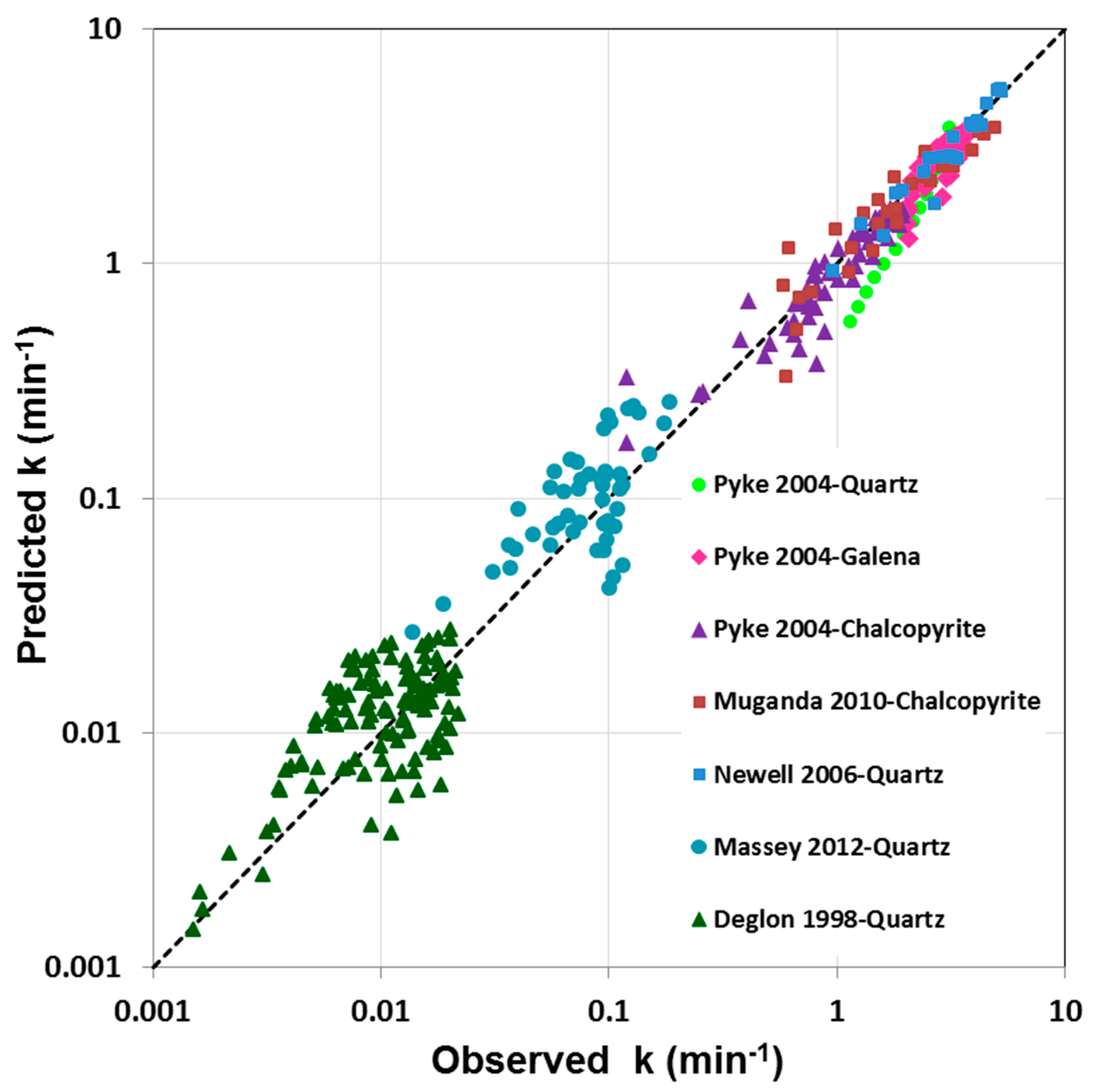
3.1. Parity Chart
3.2. Trend Prediction
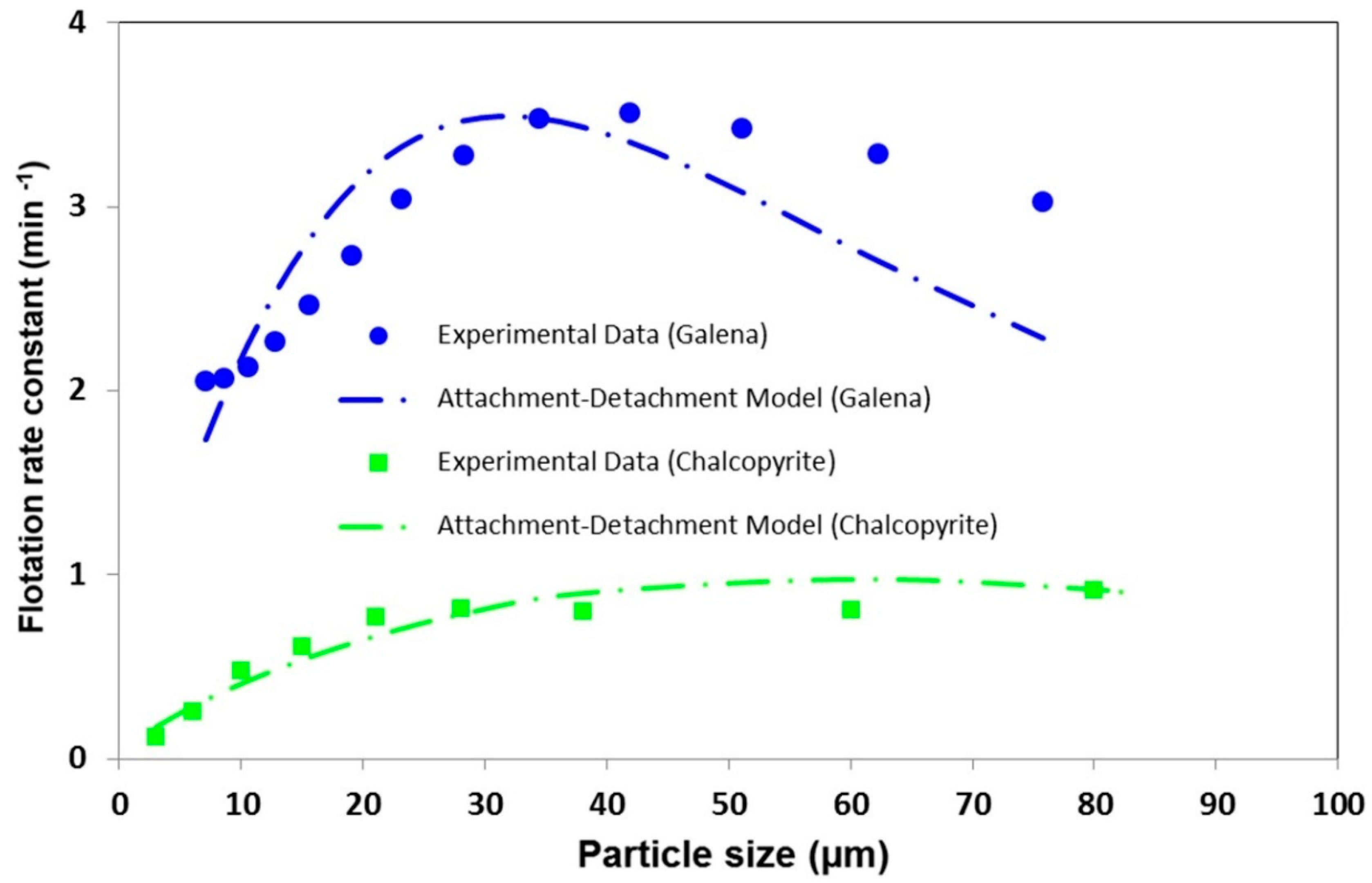
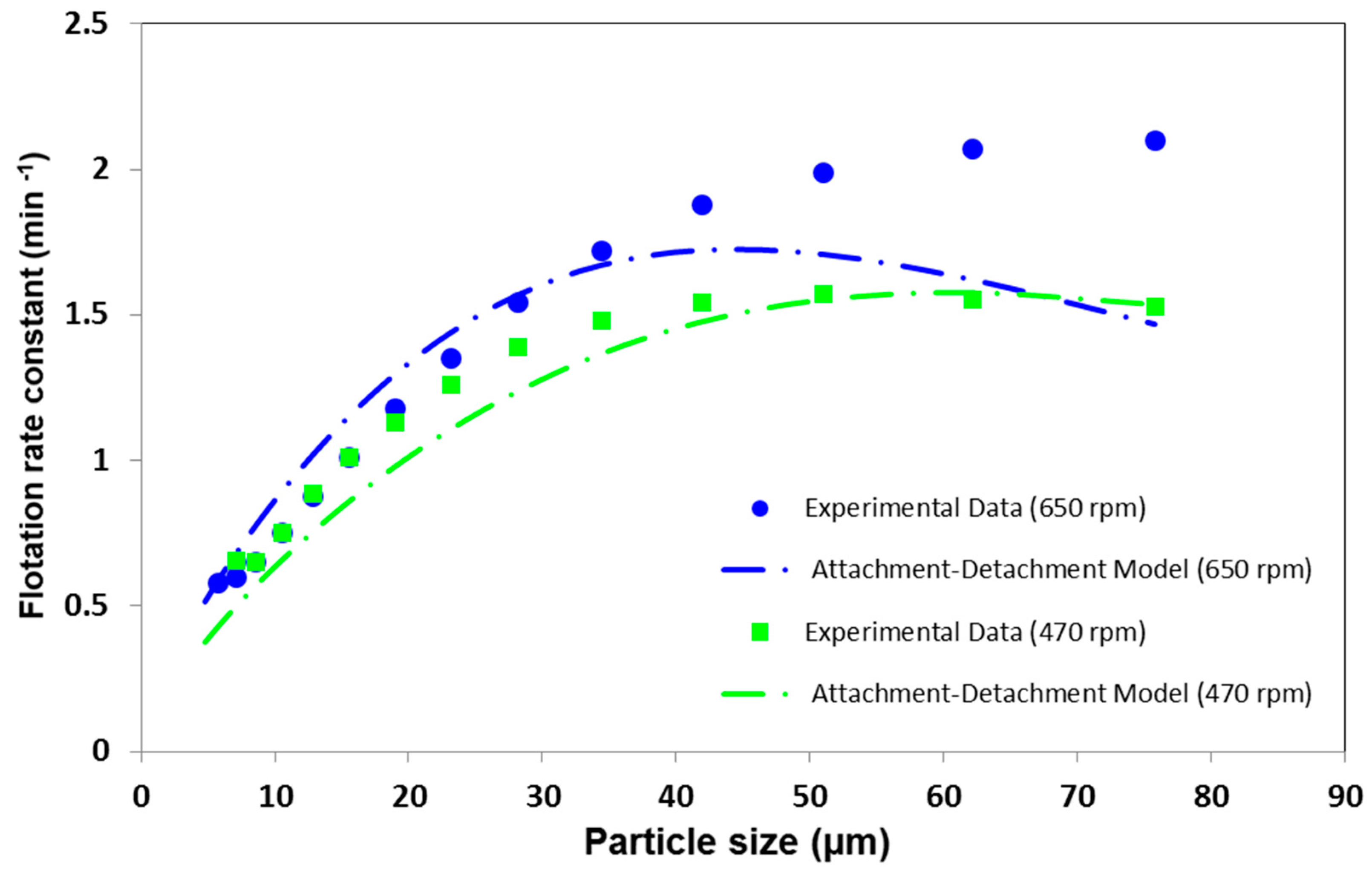
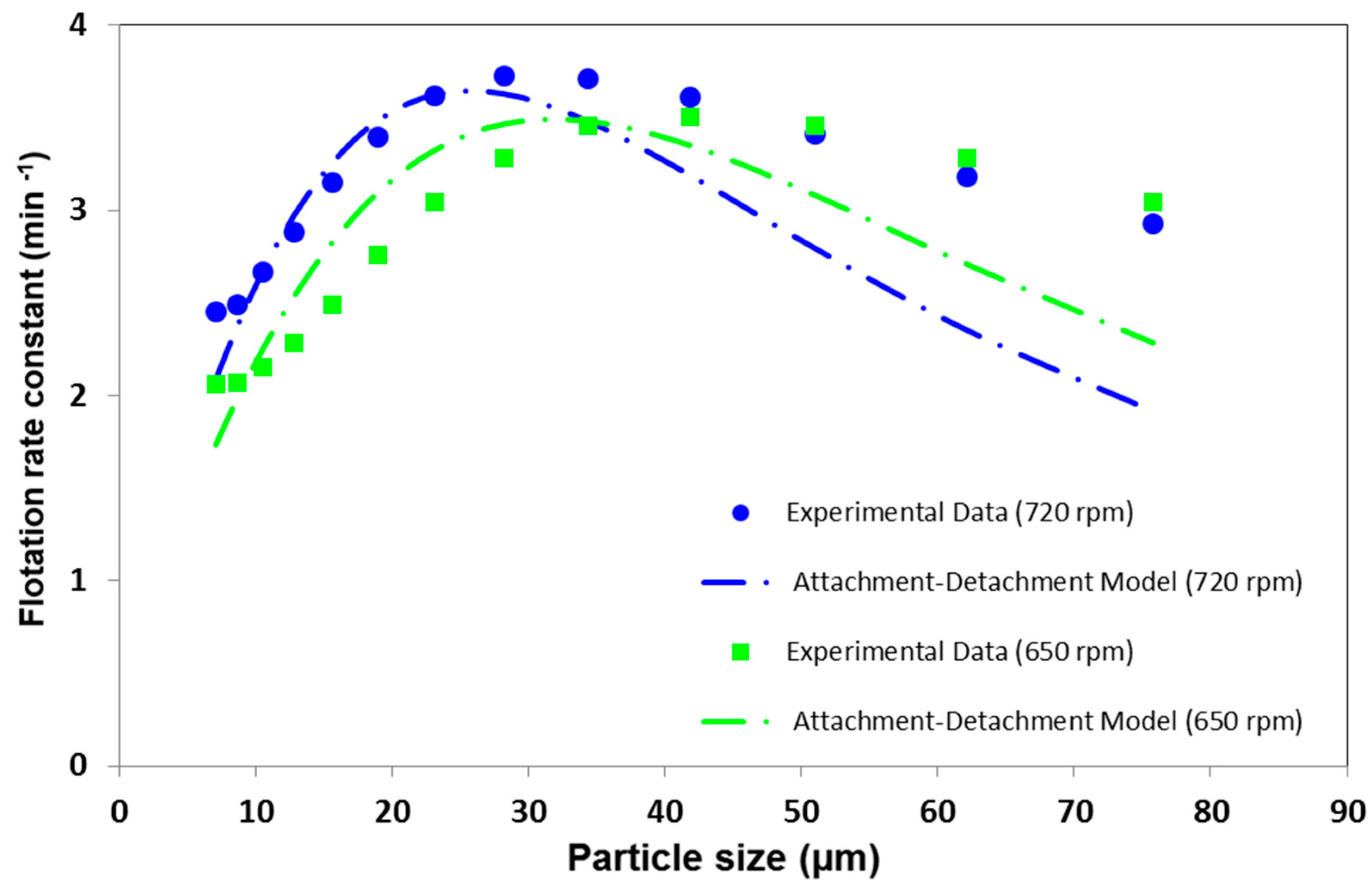
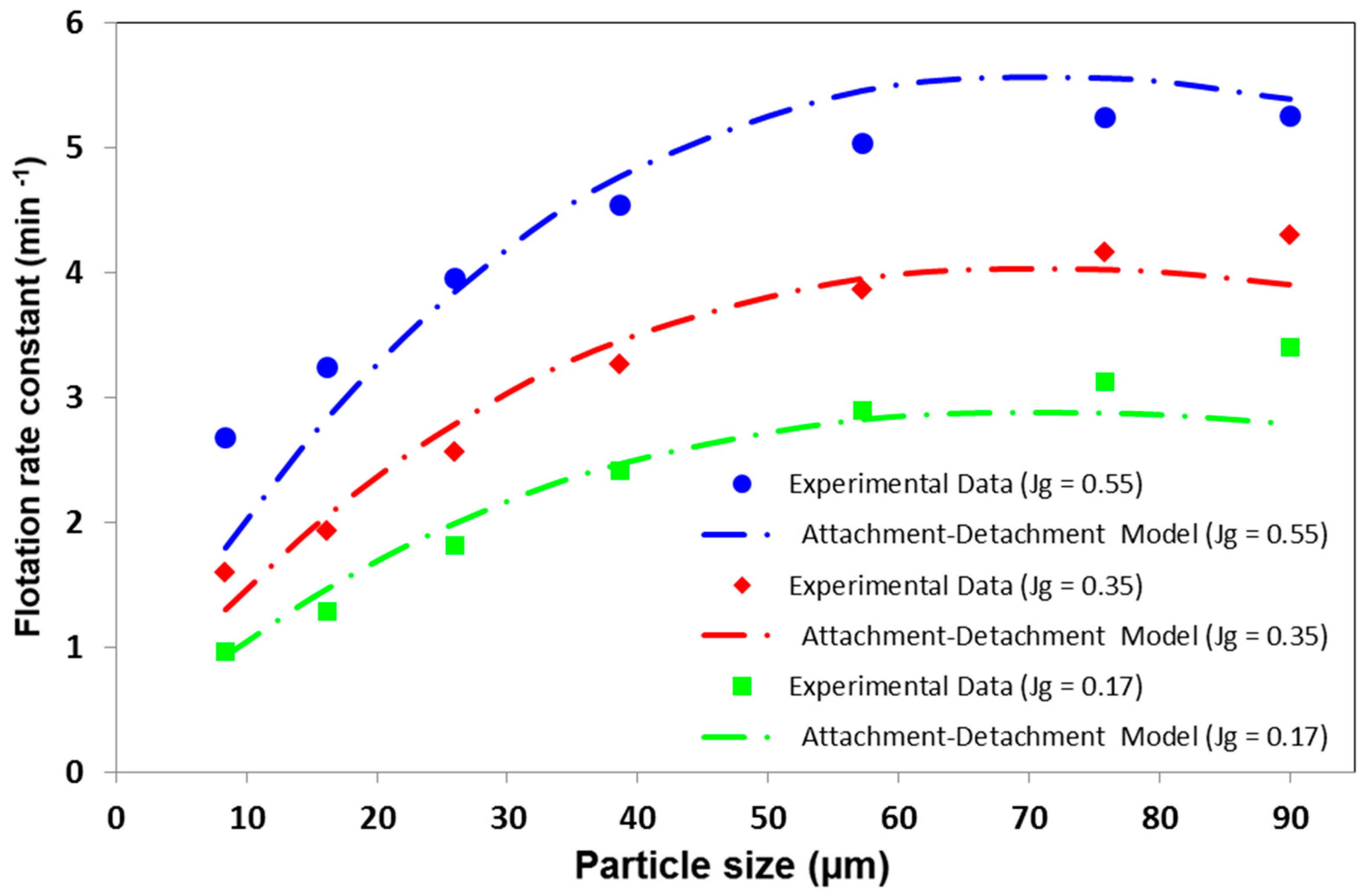
3.2.1. Particle Size
3.2.2. Contact Angle
3.2.3. Agitation/Power Input
3.2.4. Gas Flow Rate
3.3. Evaluation
4. Conclusions
Author Contributions
Funding
Conflicts of Interest
References
- Gaudin, A.M. Flotation, 2nd ed.; McGraw-Hill: New York, NY, USA, 1957. [Google Scholar]
- Bascur, O.A.; Herbst, J.A. Dynamic Modeling of a Flotation Cell with a View toward Automatic Control. CIM Bull. 1982, 75, 111–122. [Google Scholar]
- Deng, H.; Mehta, R.K.; Warren, G.W. Numerical modeling of flows in flotation columns. Int. J. Miner. Process. 1996, 48, 61–72. [Google Scholar] [CrossRef]
- Pyke, B.L.; Duan, J.; Fornasiero, D.; Ralston, J. From turbulence and collision to attachment and detachment: A general flotation model. In Flotation and Flocculation from Fundamentals to Applications; International Workshop on Flotation and Flocculation: Kailua-Kona, HI, USA, 2002; pp. 77–89. [Google Scholar]
- Pyke, B.; Fornasiero, D.; Ralston, J. Bubble particle heterocoagulation under turbulent conditions. J. Colloid Interface Sci. 2003, 265, 141–151. [Google Scholar] [CrossRef]
- Bloom, F.; Heindel, T.J. Modelling flotation separation in a semi-batch Processing. Chem. Eng. Sci. 2003, 58, 353–365. [Google Scholar] [CrossRef]
- Safari, M.; Deglon, D. An Attachment-Detachment Kinetic Model for the Effect of Energy Input on Flotation. Miner. Eng. 2018, 117, 8–13. [Google Scholar] [CrossRef]
- Dobby, G.S.; Savassi, O.N. An Advanced Modelling Technique for Scale-Up of Batch Flotation Results to Plant Metallurgical Performance. In Centenary of Flotation Symposium; AusIMM: Melbourne, Australia, 2005. [Google Scholar]
- Sherrell, I.; Yoon, R.H. Development of a turbulent flotation model. In Centenary of Flotation Symposium; AusIMM: Melbourne, Australia, 2005. [Google Scholar]
- Barnwal, J.P.; Majumder, A.K.; Govindarajan, B.; Rao, T. Modeling of coal flotation in a batch and continuous cell operation, Part 1-kinetic approach. Coal Prep. 2006, 26, 123–136. [Google Scholar] [CrossRef]
- Koh, P.; Smith, L. Experimental validation of a flotation cell model. In Proceedings of the 25th International Mineral Processing Congress (IMPC 2010), Brisbane, Australia, 6–10 September 2010. [Google Scholar]
- Goel, S.; Jameson, G.J. Detachment of particles from bubbles in an agitated vessel. Miner. Eng. 2012, 36–38, 324–330. [Google Scholar] [CrossRef]
- Karimi, M.; Akdogan, G.; Bradshaw, S.M. A computational fluid dynamics model for the flotation rate constant, Part II: Model validation. Miner. Eng. 2014, 69, 214–222. [Google Scholar] [CrossRef]
- Hoseinian, F.S.; Rezai, B.; Kowsari, E.; Safari, M. A hybrid neural network/genetic algorithm to predict Zn(II) removal by ion flotation. Sep. Sci. Technol. 2020, 55, 1197–1206. [Google Scholar] [CrossRef]
- Hoseinian, F.S.; Rezai, B.; Safari, M. A new kinetic model for zinc ion removal from synthetic wastewater. In Proceedings of the 10th European Metallurgical Conference (EMC 2019), Düsseldorf, Germany, 23–26 June 2019; pp. 1409–1416. [Google Scholar]
- Deglon, D. A novel attachment—detachment kinetic model. In Flotation and Flocculation—From Fundamentals to Applications; International Workshop on Flotation and Flocculation: Kailua-Kona, HI, USA, 2002; pp. 109–116. [Google Scholar]
- Safari, M.; Harris, M.C.; Deglon, D.A.; Filho, L.L.; Testa, F. The effect of energy input on flotation kinetics. Int. J. Miner. Process. 2016, 156, 108–115. [Google Scholar] [CrossRef]
- Deglon, D.A. A Hydrodynamic Investigation of Fine Particle Flotation in a Batch Flotation Cell. Ph.D. Thesis, Department of Chemical Engineering, University of Cape Town, Cape Town, South Africa, 1998. [Google Scholar]
- Pyke, B. Bubble–Particle Capture in Turbulent Flotation Systems. Ph.D. Thesis, Ian Wark Research Institute, University of South Australia, Mawson Lakes, Australia, 2004. [Google Scholar]
- Newell, R. Hydrodynamics and Scale-Up in Rushton Turbine Flotation Cells. Ph.D. Thesis, Ian Wark Research Institute, University of South Australia, Mawson Lakes, Australia, 2006. [Google Scholar]
- Muganda, S.; Zanin, M.; Grano, S.R. Influence of particle size and contact angle on the flotation of chalcopyrite in a laboratory batch flotation cell. Int. J. Miner. Process. 2011, 98, 150–162. [Google Scholar] [CrossRef]
- Massey, W.T.; Harris, M.C.; Deglon, D.A. The effect of energy input on the flotation of quartz in an oscillating grid flotation cell. Miner. Eng. 2012, 36–38, 145–151. [Google Scholar] [CrossRef]
- Safari, M.; Hoseinian, F.S.; Deglon, D.; Filho, K.L.L.; Souza, T. Investigation of the reverse flotation of iron ore in three different flotation cells: Mechanical, oscillating grid and pneumatic. Miner. Eng. 2020, 150, 106283. [Google Scholar] [CrossRef]
- Tabosa, E. The Effect of Cell Hydrodynamics on Flotation Kinetics. Ph.D. Thesis, University of Queensland, Brisbane, Australia, 2012. [Google Scholar]
- Hoseinian, F.S.; Rezai, B.; Safari, M.; DADeglon Kowsari, E. Effect of hydrodynamic parameters on nickel removal rate from wastewater by ion flotation. J. Environ. Manag. 2019, 244, 408–414. [Google Scholar] [CrossRef] [PubMed]
- Safari, M.; Harris, M.; Deglon, D. The effect of energy input on the flotation of a platinum ore in a pilot-scale oscillating grid flotation cell. Miner. Eng. 2017, 110, 69–74. [Google Scholar] [CrossRef]
- Tabosa, E.; Runge, K.; Holtham, P.; Duffy, K. Improving flotation energy efficiency by optimizing cell hydrodynamics. Miner. Eng. 2016, 96–97, 194–202. [Google Scholar] [CrossRef]
- Hoseinian, F.S.; Rezai, B.; Kowsari, E.; Safari, M. Effect of impeller speed on the Ni(II) ion flotation. Geosyst. Eng. 2018, 22, 161–168. [Google Scholar] [CrossRef]
- Safari, M.; Harris, M.; Deglon, D. The effect of energy input on the flotation kinetics of galena in an oscillating grid flotation cell. In Proceedings of the 27th International Mineral Processing Congress (IMPC 2014), Santiago, Chile, 20–24 October 2014. [Google Scholar]
- Testa, F.; Safari, M.; Deglon, D.; Filho, L.L. Influence of agitation intensity on flotation rate of apatite particles. Rev. Esc. Minas 2017, 70, 491–495. [Google Scholar] [CrossRef]
- Safari, M.; Hoseinian, F.S.; Deglon, D.; Filho, K.L.L.; Souza, T. Investigation of the reverse flotation of hematite in three different types of laboratory flotation cells. In Proceedings of the 29th International Mineral Processing Congress (IMPC 2018), Moscow, Russia, 17–21 September 2018; pp. 1376–1383. [Google Scholar]
- Gorain, B.K.; Franzidis, J.P.; Manlapig, E.V. Studies on impeller type, impeller speed and air flow rate in an industrial scale flotation cell. Part 4: Effect of bubble surface area flux on flotation kinetics. Miner. Eng. 1997, 10, 367–379. [Google Scholar] [CrossRef]


| Minerals | Attachment Rate Constant (ka) | Detachment Rate Constant (kd) | ||
|---|---|---|---|---|
| All Minerals | n1 | 0.72 | n1 | 2.17 |
| n2 | 0.91 | n2 | 1.33 | |
| n3 | 0.47 | n3 | −1.17 | |
| n4 | −0.77 | n4 | 0.67 | |
| n5 | 1.81 | n5 | 0.67 | |
| New Coefficients | c2* | 1.17 | c4* | 1.77 × 10⁻⁵ |
| #Units: dp (µm), db (mm), θ (°), ρ (ton/m3), ε (W/kg) | ||||
Publisher’s Note: MDPI stays neutral with regard to jurisdictional claims in published maps and institutional affiliations. |
© 2020 by the authors. Licensee MDPI, Basel, Switzerland. This article is an open access article distributed under the terms and conditions of the Creative Commons Attribution (CC BY) license (http://creativecommons.org/licenses/by/4.0/).
Share and Cite
Safari, M.; Deglon, D. Evaluation of an Attachment–Detachment Kinetic Model for Flotation. Minerals 2020, 10, 978. https://doi.org/10.3390/min10110978
Safari M, Deglon D. Evaluation of an Attachment–Detachment Kinetic Model for Flotation. Minerals. 2020; 10(11):978. https://doi.org/10.3390/min10110978
Chicago/Turabian StyleSafari, Mehdi, and David Deglon. 2020. "Evaluation of an Attachment–Detachment Kinetic Model for Flotation" Minerals 10, no. 11: 978. https://doi.org/10.3390/min10110978
APA StyleSafari, M., & Deglon, D. (2020). Evaluation of an Attachment–Detachment Kinetic Model for Flotation. Minerals, 10(11), 978. https://doi.org/10.3390/min10110978