
3D Reconstruction Framework for Multiple Remote Robots on Cloud System


Abstract
:1. Introduction
2. Related Works
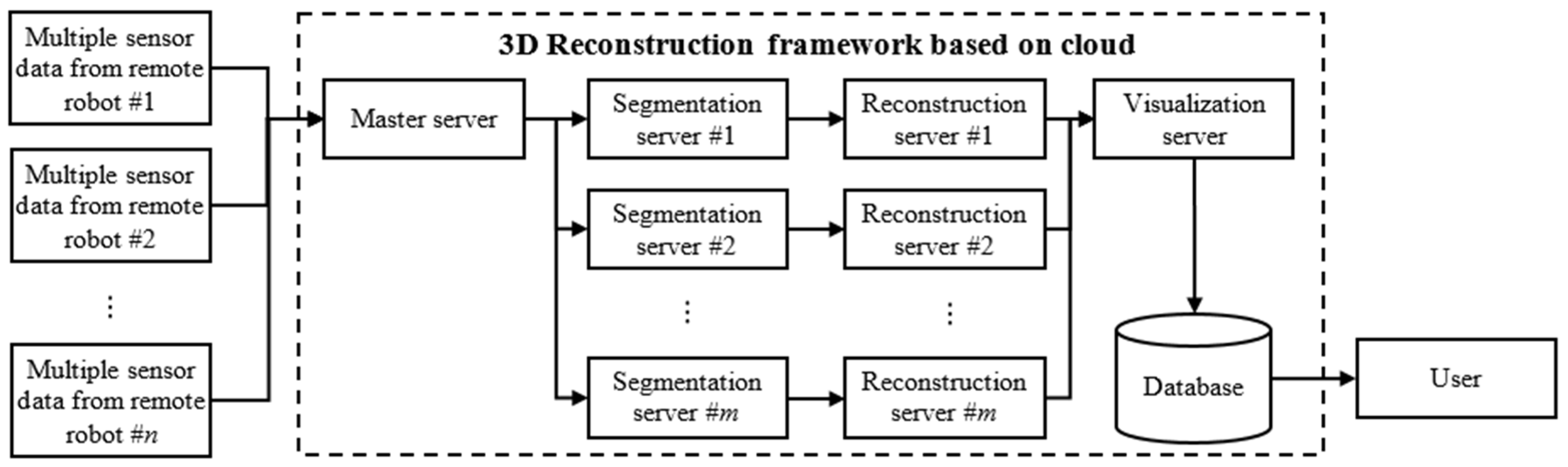
3. Framework Design
3.1. Ground Segmentation Algorithm
| Algorithm 1 Ground segmentation |
| Convert all points into global coordinate() |
| FOR EACH vertical-line IN a frame data |
| WHILE NOT (all points in the vertical-line are labeled) |
| Assign a start-ground point() |
| Find a threshold point() |
| Assign points’ label() |
| END |
| END |
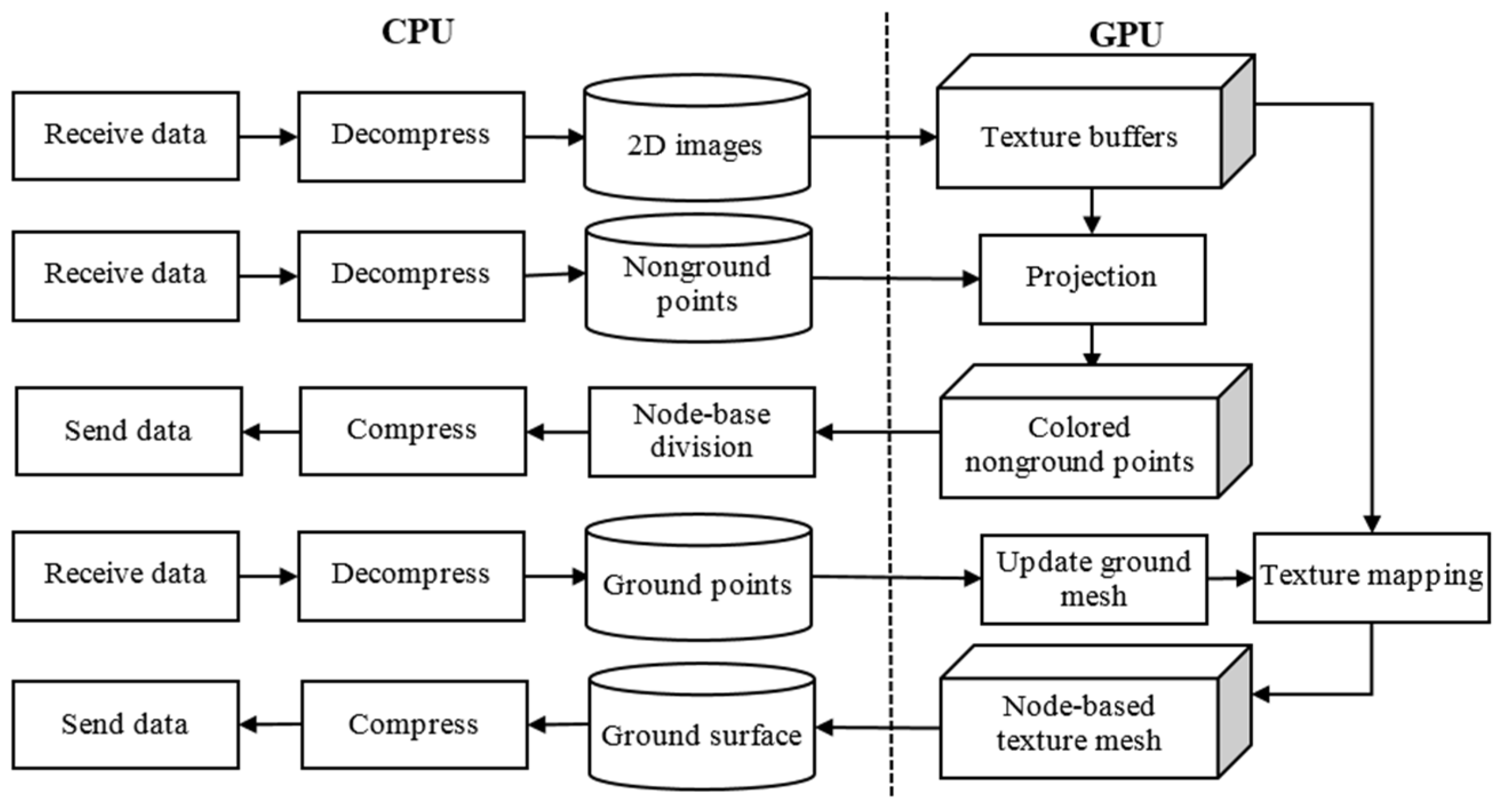
3.2. Terrain Reconstruction Algorithm
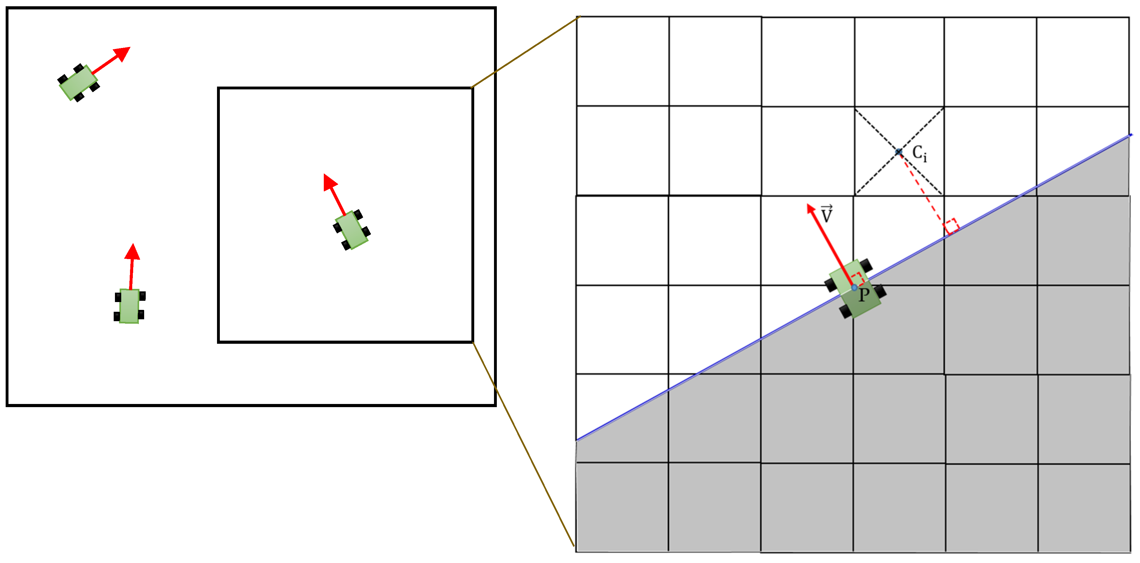
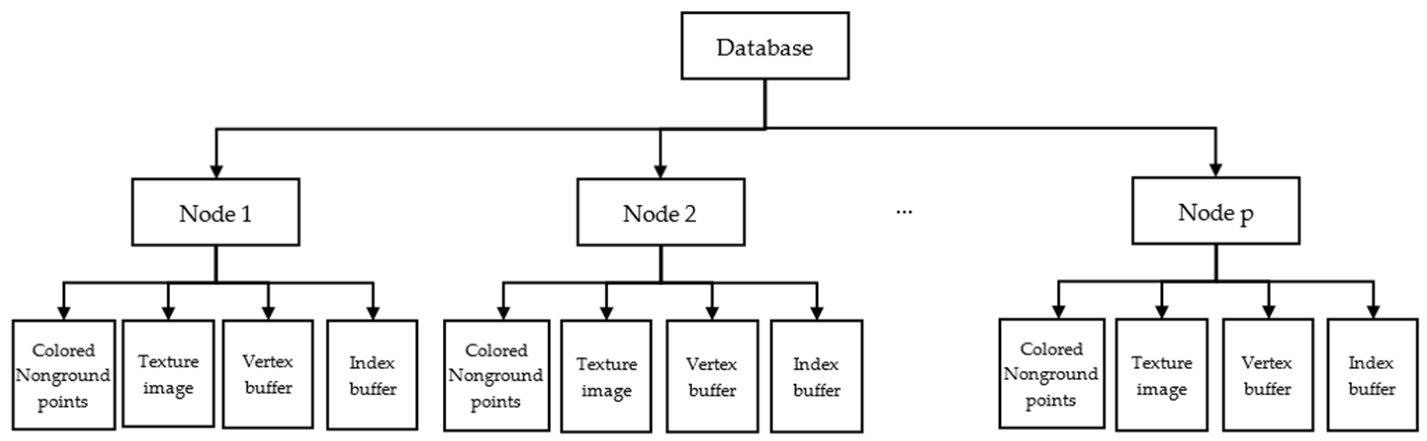
3.3. Reconstruction Data Processing
| Algorithm 2 Sending ground surface data |
| Ratio ← Number_Of_Triangles/Maximum_Triangles |
| Estimated_Ratio ← Number_Of_Triangles/Estimated_Number_Of_Triangles |
| Threshold ← Medium_Value |
| Intersection_Status ← Check intersection between orthogonal line and Node() |
| Dynamic_Increasing_Delta_1 ← (1 − Previous_Ratio)/2 |
| IF Intersection_Status = TRUE THEN |
| IF Never_Send_Data = TRUE THEN |
| Threshold ← Small_Value |
| ELSE IF (Ratio − Previous_Ratio) < Dynamic_Increasing_Delta_1 THEN |
| RETURN FALSE |
| END |
| END |
| IF Never_Send_Data = TRUE THEN |
| IF (Ratio < Threshold) OR (Estimated_Ratio < Threshold) THEN |
| RETURN FALSE |
| ELSE |
| Previous_Ratio ← Ratio |
| Never_Send_Data ← FALSE |
| END |
| ELSE |
| Dynamic_Increasing_Delta_2 ← (1 − Previous_Ratio)/4 |
| IF (Ratio − Previous_Ratio) < Dynamic_Increasing_Delta_2 THEN |
| Dist ← Distance between Node’s center and orthogonal line() |
| IF (Dist < Size_Of_Node) AND (Ratio > Previous_Ratio) THEN |
| Previous_Ratio ← Ratio |
| ELSE |
| Return FALSE |
| END |
| END |
| Previous_Ratio ← Ratio |
| END |
| END |
| Compress Data() |
| Send Data() |
| RETURN TRUE |
4. Experiments and Analysis
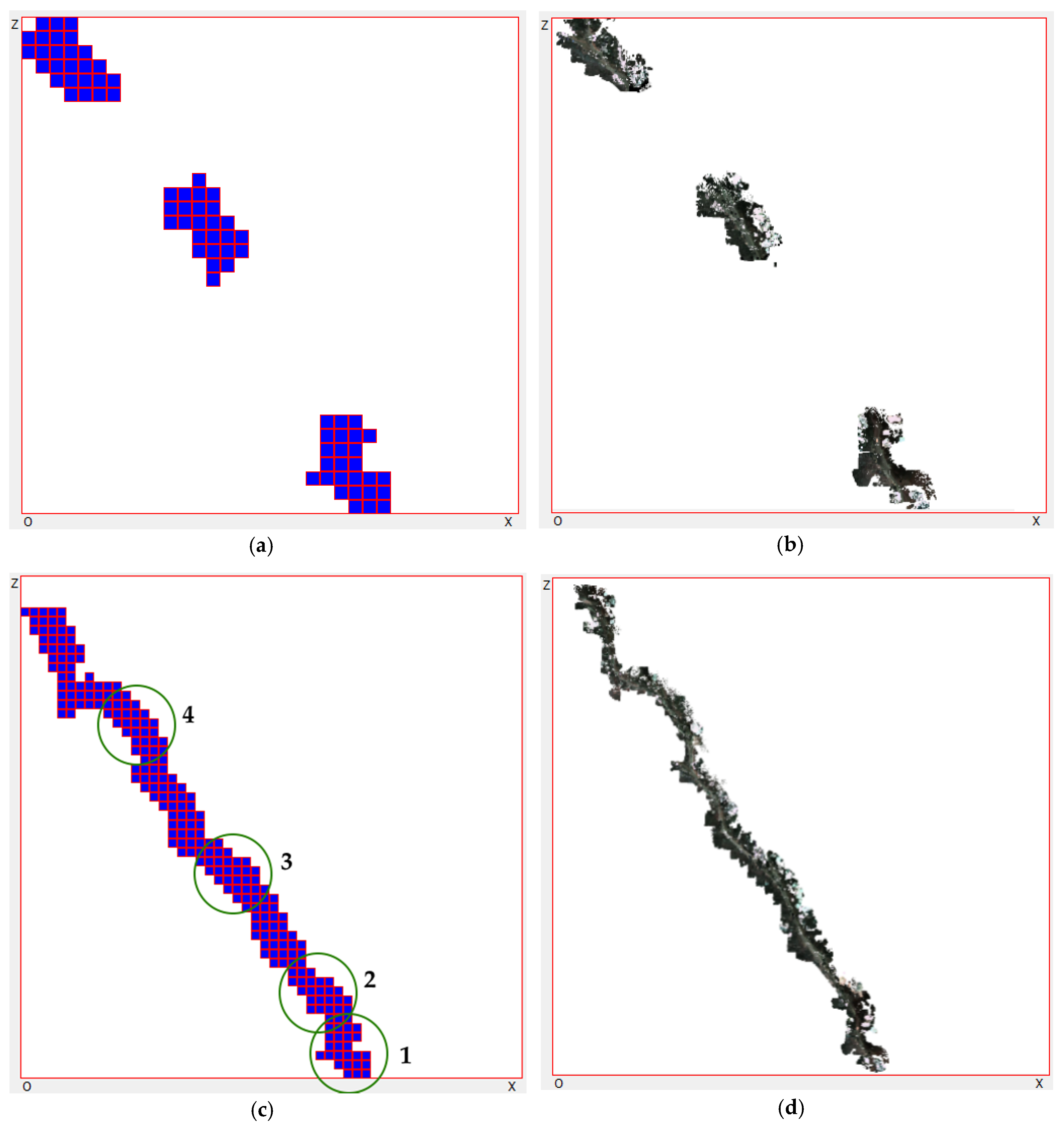
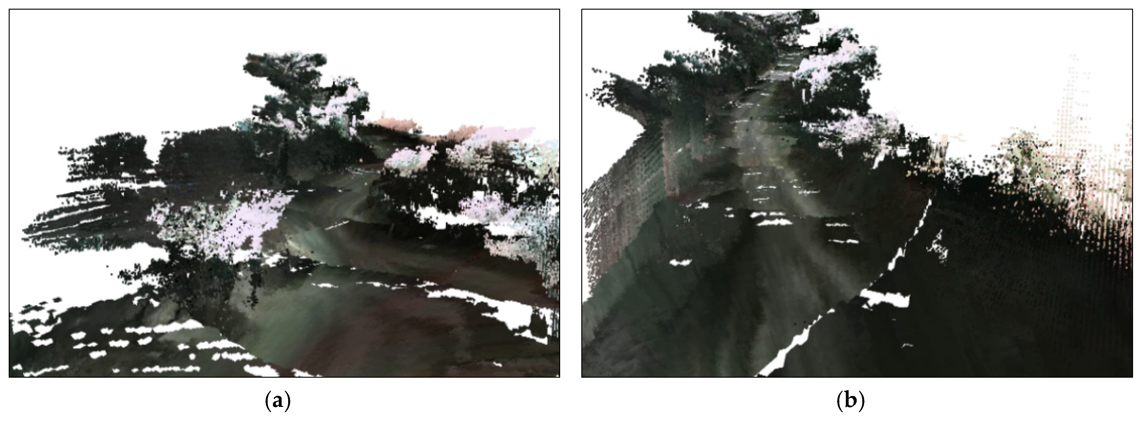
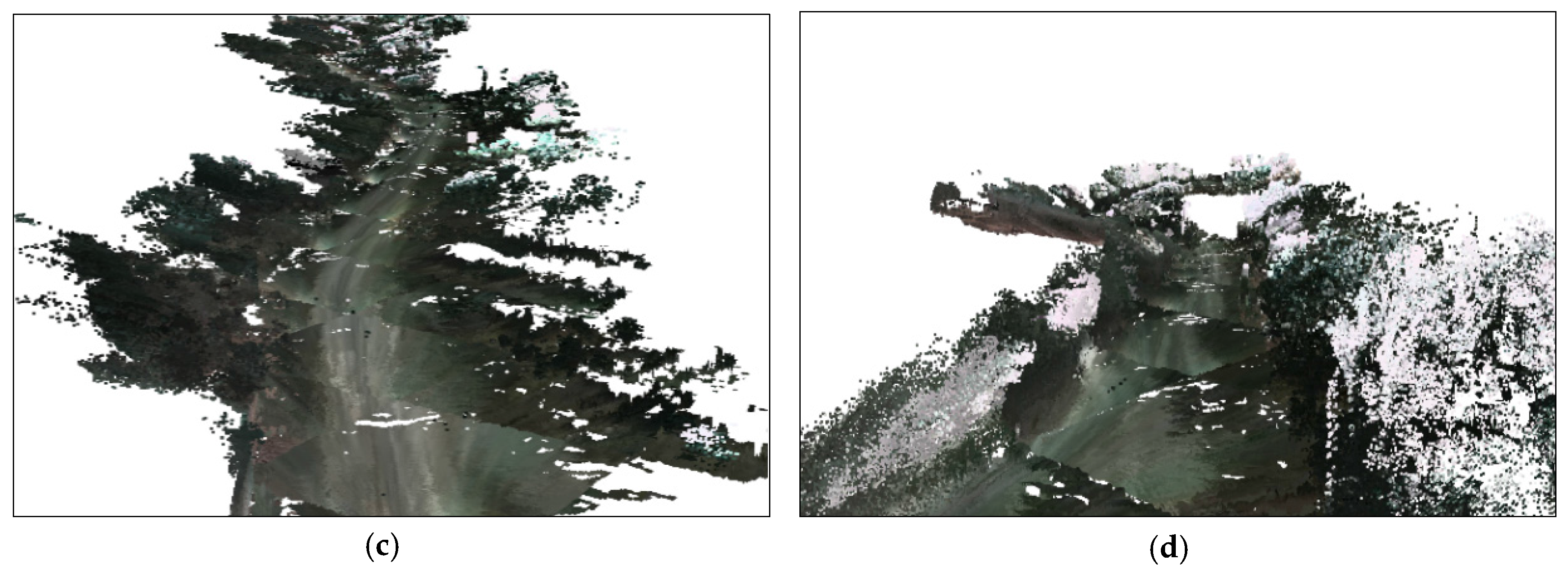
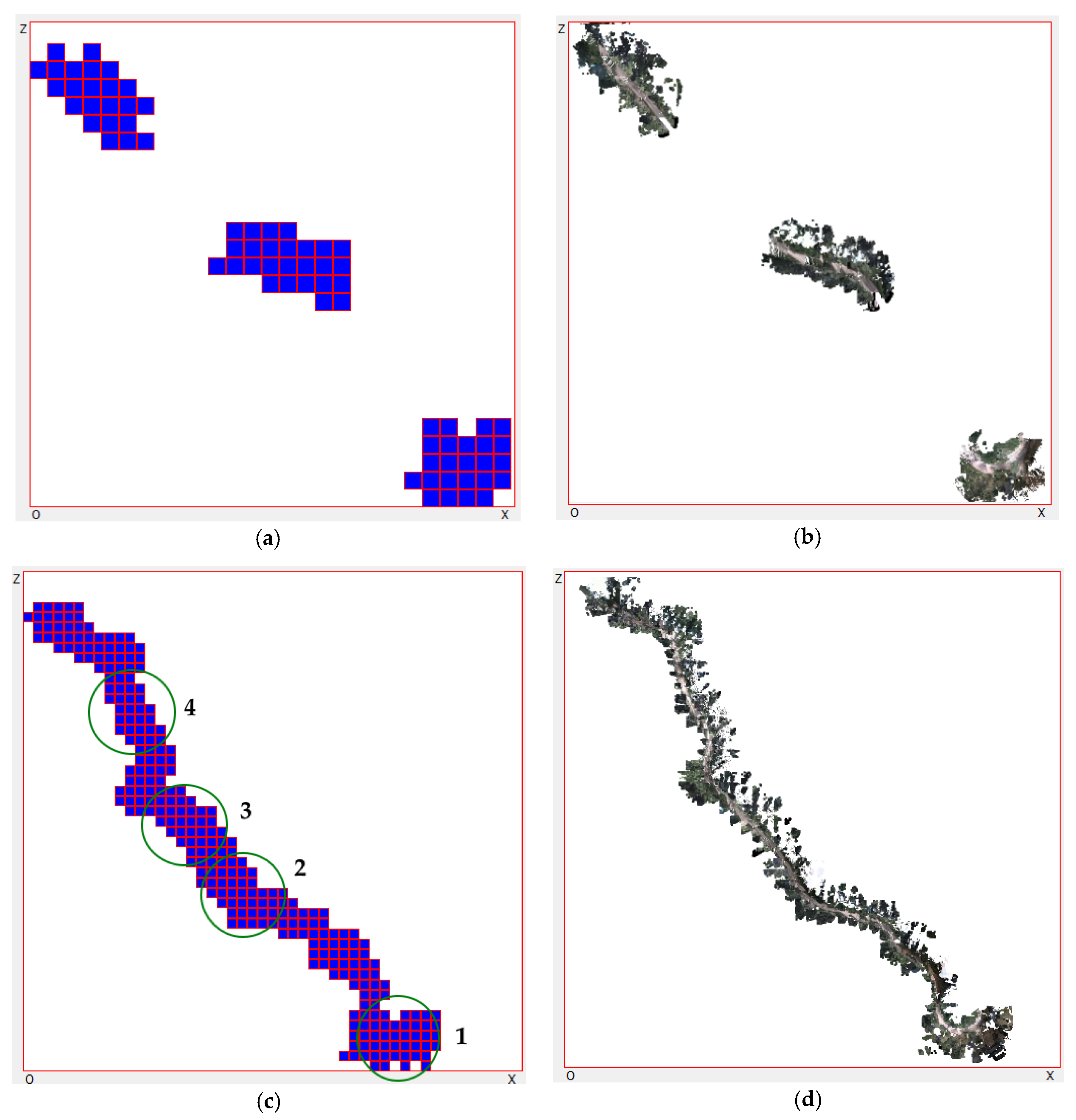
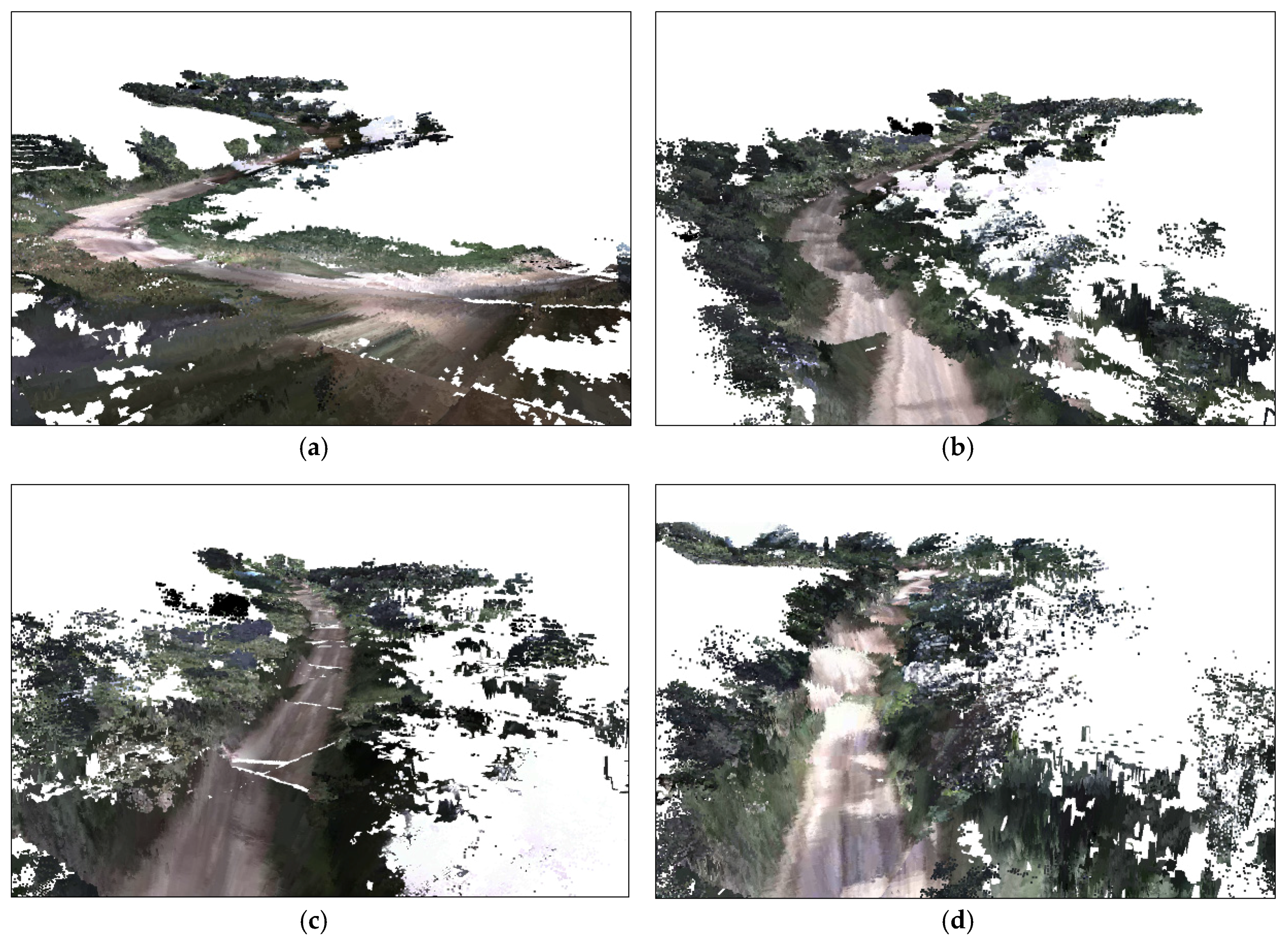
4.1. Experimental Results
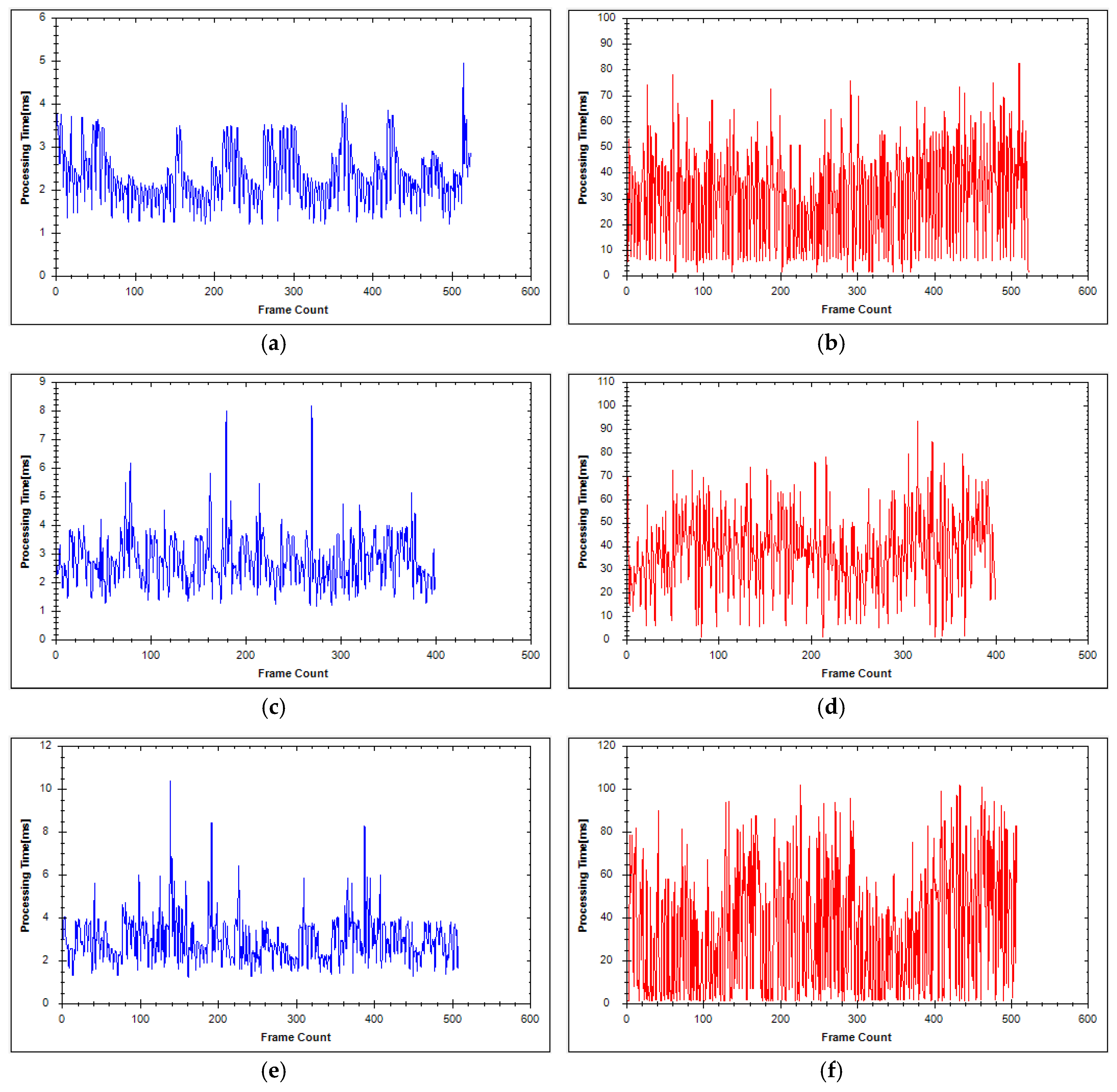
4.2. Experimental Analysis
5. Conclusions
Acknowledgments
Author Contributions
Conflicts of Interest
References
- Kamal, S.; Azurdia-Meza, C.A.; Lee, K. Suppressing the effect of ICI power using dual sinc pulses in OFDM-based systems. Int. J. Electron. Commun. 2016, 70, 953–960. [Google Scholar] [CrossRef]
- Azurdia-Meza, C.A.; Falchetti, A.; Arrano, H.F.; Kamal, S.; Lee, K. Evaluation of the improved parametric linear combination pulse in digital baseband communication systems. In Proceedings of the Information and Communication Technology Convergence (ICTC) Conference, Jeju, Korea, 28–30 October 2015; pp. 485–487. [Google Scholar]
- Kamal, S.; Azurdia-Meza, C.A.; Lee, K. Family of Nyquist-I Pulses to Enhance Orthogonal Frequency Division Multiplexing System Performance. IETE Tech. Rev. 2016, 33, 187–198. [Google Scholar] [CrossRef]
- Azurdia-Meza, C.A.; Kamal, S.; Lee, K. BER enhancement of OFDM-based systems using the improved parametric linear combination pulse. In Proceedings of the Information and Communication Technology Convergence (ICTC) Conference, Jeju, Korea, 28–30 October 2015; pp. 743–745. [Google Scholar]
- Kamal, S.; Azurdia-Meza, C.A.; Lee, K. Subsiding OOB Emission and ICI power using iPOWER pulse in OFDM systems. Adv. Electr. Comput. Eng. 2016, 16, 79–86. [Google Scholar] [CrossRef]
- Kamal, S.; Azurdia-Meza, C.A.; Lee, K. Nyquist-I pulses designed to suppress the effect of ICI power in OFDM systems. In Proceedings of the Wireless Communications and Mobile Computing Conference (IWCMC) International Conference, Dubrovnik, Croatia, 24–28 August 2015; pp. 1412–1417. [Google Scholar]
- Jalal, A.; Sarif, N.; Kim, J.T.; Kim, T.S. Human activity recognition via recognized body parts of human depth silhouettes for residents monitoring services at smart homes. Indoor Built Environ. 2013, 22, 271–279. [Google Scholar] [CrossRef]
- Jalal, A.; Kim, Y.H.; Kim, Y.J.; Kamal, S.; Kim, D. Robust human activity recognition from depth video using spatiotemporal multi-fused features. Pattern Recognit. 2017, 61, 295–308. [Google Scholar] [CrossRef]
- Jalal, A.; Kamal, S.; Kim, D. A depth video sensor-based life-logging human activity recognition system for elderly care in smart indoor environments. Sensors 2014, 14, 11735–11759. [Google Scholar] [CrossRef] [PubMed]
- Jalal, A.; Kamal, S.; Kim, D. A depth video-based human detection and activity recognition using multi-features and embedded hidden Markov models for health care monitoring systems. Int. J. Interact. Multimed. Artif. Intell. 2017, 4, 54–62. [Google Scholar] [CrossRef]
- Tian, G.; Meng, D. Failure rules based mode resource provision policy for cloud computing. In Proceedings of the 2010 International Symposium on Parallel and Distributed Processing with Applications (ISPA), Taipei, Taiwan, 6–9 September 2010; pp. 397–404. [Google Scholar]
- Jalal, A.; Kim, D. Global security using human face understanding under vision ubiquitous architecture system. World Acad. Sci. Eng. Technol. 2006, 13, 7–11. [Google Scholar]
- Puwein, J.; Ballan, L.; Ziegler, R.; Pollefeys, M. Joint camera pose estimation and 3D human pose estimation in a multi-camera setup. In Proceedings of the IEEE Asian Conference on Computer Vision (ACCV), Singapore, 1–5 November 2014; pp. 473–487. [Google Scholar]
- Jalal, A.; Kim, Y.; Kim, D. Ridge body parts features for human pose estimation and recognition from RGB-D video data. In Proceedings of the IEEE International Conference on Computing, Communication and Networking Technologies, Hefei, China, 11–13 July 2014; pp. 1–6. [Google Scholar]
- Jalal, A.; Kamal, S.; Kim, D. Human depth sensors-based activity recognition using spatiotemporal features and hidden markov model for smart environments. J. Comput. Netw. Commun. 2016, 2016. [Google Scholar] [CrossRef]
- Bodor, R.; Morlok, R.; Papanikolopoulos, N. Dual-camera system for multi-level activity recognition. In Proceedings of the 2004 IEEE/RSJ International Conference on Intelligent Robots and Systems (IROS 2004), Sendai, Japan, 28 September–2 October 2004. [Google Scholar]
- Kamal, S.; Jalal, A.; Kim, D. Depth images-based human detection, tracking and activity recognition using spatiotemporal features and modified HMM. J. Electr. Eng. Technol. 2016, 11, 1857–1862. [Google Scholar] [CrossRef]
- Jalal, A.; Kamal, S.; Kim, D. Individual detection-tracking-recognition using depth activity images. In Proceedings of the 12th IEEE International Conference on Ubiquitous Robots and Ambient Intelligence, Goyang, Korea, 28–30 October 2015; pp. 450–455. [Google Scholar]
- Farooq, A.; Jalal, A.; Kamal, S. Dense RGB-D Map-Based Human Tracking and Activity Recognition using Skin Joints Features and Self-Organizing Map. KSII Trans. Int. Inf. Syst. 2015, 9, 1856–1869. [Google Scholar]
- Jalal, A.; Kamal, S.; Kim, D. Depth Map-based Human Activity Tracking and Recognition Using Body Joints Features and Self-Organized Map. In Proceedings of the IEEE International Conference on Computing, Communication and Networking Technologies, Hefei, China, 11–13 July 2014. [Google Scholar]
- Jalal, A.; Kamal, S. Real-Time Life Logging via a Depth Silhouette-based Human Activity Recognition System for Smart Home Services. In Proceedings of the IEEE International Conference on Advanced Video and Signal-Based Surveillance, Seoul, Korea, 26–29 August 2014; pp. 74–80. [Google Scholar]
- Kamal, S.; Jalal, A. A hybrid feature extraction approach for human detection, tracking and activity recognition using depth sensors. Arab. J. Sci. Eng. 2016, 41, 1043–1051. [Google Scholar] [CrossRef]
- Jalal, A.; Kamal, S.; Farooq, A.; Kim, D. A spatiotemporal motion variation features extraction approach for human tracking and pose-based action recognition. In Proceedings of the IEEE International Conference on Informatics, Electronics and Vision, Fukuoka, Japan, 15–17 June 2015. [Google Scholar]
- Jalal, A.; Kim, S. The Mechanism of Edge Detection using the Block Matching Criteria for the Motion Estimation. In Proceedings of the Conference on Human Computer Interaction, Las Vegas, NV, USA, 22–27 July 2005; pp. 484–489. [Google Scholar]
- Jalal, A.; Zeb, M.A. Security and QoS Optimization for distributed real time environment. In Proceedings of the IEEE International Conference on Computer and Information Technology, Dhaka, Bangladesh, 27–29 December 2007; pp. 369–374. [Google Scholar]
- Munir, K. Security model for cloud database as a service (DBaaS). In Proceedings of the IEEE Conference on Cloud Technologies and Applications, Marrakech, Morocco, 2–4 June 2015. [Google Scholar]
- Jalal, A.; IjazUddin. Security architecture for third generation (3G) using GMHS cellular network. In Proceedings of the IEEE International Conference on Emerging Technologies, Islamabad, Pakistan, 12–13 November 2007. [Google Scholar]
- Kar, J.; Mishra, M.R. Mitigating Threats and Security Metrics in Cloud Computing. J. Inf. Process. Syst. 2016, 12, 226–233. [Google Scholar]
- Zhu, W.; Lee, C. A Security Protection Framework for Cloud Computing. J. Inf. Process. Syst. 2016, 12. [Google Scholar] [CrossRef]
- Izadi, S.; Kim, D.; Hilliges, O.; Molyneaux, D.; Newcombe, R.; Kohli, P.; Shotton, J.; Hodges, S.; Freeman, D.; Davison, A.; et al. KinectFusion: Real-time 3D Reconstruction and Interaction Using a Moving Depth Camera. In Proceedings of the 24th Annual ACM Symposium on User Interface Software and Technology, Santa Barbara, CA, USA, 16–19 October 2011; pp. 559–568. [Google Scholar]
- Popescu, C.R.; Lungu, A. Real-Time 3D Reconstruction Using a Kinect Sensor. In Computer Science and Information Technology; Horizon Research Publishing: San Jose, CA, USA, 2014; Volume 2, pp. 95–99. [Google Scholar]
- Khatamian, A.; Arabnia, H.R. Survey on 3D Surface Reconstruction. J. Inf. Process. Syst. 2016, 12, 338–357. [Google Scholar]
- Huber, D.; Herman, H.; Kelly, A.; Rander, P.; Ziglar, J. Real-time Photo-realistic Visualization of 3D Environments for Enhanced Tele-operation of Vehicles. In Proceedings of the IEEE International Conference on Computer Vision Workshops (ICCV Workshops), Kyoto, Japan, 27 September–4 October 2009; pp. 1518–1525. [Google Scholar]
- Kelly, A.; Capstick, E.; Huber, D.; Herman, H.; Rander, P.; Warner, R. Real-Time Photorealistic Virtualized Reality Interface For Remote Mobile Robot Control. In Springer Tracts in Advanced Robotics; Springer: New York, NY, USA, 2011; Volume 70, pp. 211–226. [Google Scholar]
- Song, W.; Cho, K. Real-time terrain reconstruction using 3D flag map for point clouds. Multimed. Tools Appl. 2013, 74, 3459–3475. [Google Scholar] [CrossRef]
- Song, W.; Cho, S.; Cho, K.; Um, K.; Won, C.S.; Sim, S. Traversable Ground Surface Segmentation and Modeling for Real-Time Mobile Mapping. Int. J. Distrib. Sens. Netw. 2014, 10. [Google Scholar] [CrossRef]
- Chu, P.; Cho, S.; Cho, K. Fast ground segmentation for LIDAR Point Cloud. In Proceedings of the 5th International Conference on Ubiquitous Computing Application and Wireless Sensor Network (UCAWSN-16), Jeju, Korea, 6–8 July 2016. [Google Scholar]
- Hernández, J.; Marcotegui, B. Point Cloud Segmentation towards Urban Ground Modeling. In Proceedings of the IEEE Urban Remote Sensing Event, Shanghai, China, 20–22 May 2009; pp. 1–5. [Google Scholar]
- Moosmann, F.; Pink, O.; Stiller, C. Segmentation of 3D Lidar Data in non-flat Urban Environments using a Local Convexity Criterion. In Proceedings of the IEEE Intelligent Vehicles Symposium, Xi’an, China, 3–5 June 2009; pp. 215–220. [Google Scholar]
- Douillard, B.; Underwood, J.; Kuntz, N.; Vlaskine, V.; Quadros, A.; Morton, P.; Frenkel, A. On the Segmentation of 3D LIDAR Point Clouds. In Proceedings of the IEEE International Conference on Robotics and Automation, Shanghai, China, 9–13 May 2011; pp. 2798–2805. [Google Scholar]
- Lin, X.; Zhang, J. Segmentation-based ground points detection from mobile laser scanning point cloud. In Proceedings of the 2015 International Workshop on Image and Data Fusion, Kona, HI, USA, 21–23 July 2015; pp. 99–102. [Google Scholar]
- Cho, S.; Kim, J.; Ikram, W.; Cho, K.; Jeong, Y.; Um, K.; Sim, S. Sloped Terrain Segmentation for Autonomous Drive Using Sparse 3D Point Cloud. Sci. World J. 2014, 2014. [Google Scholar] [CrossRef] [PubMed]
- Tomori, Z.; Gargalik, R.; Hrmo, I. Active segmentation in 3d using kinect sensor. In Proceedings of the International Conference Computer Graphics Visualization and Computer Vision, Plzen, Czech, 25–28 June 2012; pp. 163–167. [Google Scholar]
- Paquette, L.; Stampfler, R.; Dube, Y.; Roussel, M. A new approach to robot orientation by orthogonal lines. In Proceedings of the CVPR’88, Computer Society Conference on Computer Vision and Pattern Recognition, Ann Arbor, MI, USA, 5–9 June 1988; pp. 89–92. [Google Scholar]
- Brüggemann, B.; Schulz, D. Coordinated Navigation of Multi-Robot Systems with Binary Constraints. In Proceedings of the 2010 IEEE/RSJ International Conference on Intelligent Robots and Systems, Taipei, Taiwan, 18–22 October 2010. [Google Scholar]
- Brüggemann, B.; Brunner, M.; Schulz, D. Spatially constrained coordinated navigation for a multi-robot system. Ad Hoc Netw. 2012, 11, 1919–1930. [Google Scholar] [CrossRef]
- Mohanarajah, G.; Usenko, V.; Singh, M.; Andrea, R.D.; Waibel, M. Cloud-based collaborative 3D mapping in real-time with low-cost robots. IEEE Trans. Autom. Sci. Eng. 2015, 12, 423–431. [Google Scholar] [CrossRef]
- Jessup, J.; Givigi, S.N.; Beaulieu, A. Robust and Efficient Multi-Robot 3D Mapping with Octree Based Occupancy Grids. In Proceedings of the IEEE International Conference on Systems, Man, and Cybernetics (SMC), San Diego, CA, USA, 5–8 October 2014; pp. 3996–4001. [Google Scholar]
- Riazuelo, L.; Civera, J.; Montiel, J.M.M. C2TAM: A Cloud framework for cooperative tracking and mapping. Robot. Auton. Syst. 2014, 62, 401–413. [Google Scholar] [CrossRef]
- Yoon, J.H.; Park, H.S. A Cloud-based Integrated Development Environment for Robot Software Development. J. Inst. Control Robot. Syst. 2015, 21, 173–178. [Google Scholar] [CrossRef]
- Lee, J.; Choi, B.G.; Bae, J.H. Cloudboard: A Cloud-Based Knowledge Sharing and Control System. KIPS Trans. Softw. Data Eng. 2015, 4, 135–142. [Google Scholar] [CrossRef]
- Sim, S.; Sock, J.; Kwak, K. Indirect Correspondence-Based Robust Extrinsic Calibration of LiDAR and Camera. Sensors 2016, 16. [Google Scholar] [CrossRef] [PubMed]
- Gu, Y.; Grossman, R.L. UDT: UDP-based data transfer for high-speed wide area networks. Comput. Netw. 2007, 51, 1777–1799. [Google Scholar] [CrossRef]
- Jiang, Y.; Li, Y.; Ban, D.; Xu, Y. Frame buffer compression without color information loss. In Proceedings of the 12th IEEE International Conference on Computer and Information Technology, Chengdu, China, 27–29 October 2012. [Google Scholar]
- Jalal, A.; Kim, S. Advanced performance achievement using multi-algorithmic approach of video transcoder for low bit rate wireless communication. ICGST Int. J. Graph. Vis. Image Process. 2005, 5, 27–32. [Google Scholar]
- Jalal, A.; Rasheed, Y.A. Collaboration achievement along with performance maintenance in video streaming. In Proceedings of the IEEE International Conference on Interactive Computer Aided Learning, Villach, Austria, 26–28 September 2007. [Google Scholar]
- Maxwell, C.A.; Jayavant, R. Digital images, compression, decompression and your system. In Proceedings of the Conference Record WESCON/94, Anaheim, CA, USA, 27–29 September 1994; pp. 144–147. [Google Scholar]
- ZLIB. Available online: http://www.zlib.net (accessed on 10 September 2016).


| PC | Central Processing Unit (CPU) | Random-Access Memory (RAM) (GB) | Graphics Processing Unit (GPU) | Video RAM (VRAM) (GB) |
|---|---|---|---|---|
| Master server | Core i7, 2.93 GHz | 12 | - | - |
| Segmentation sever 1 | Core i7-2600K, 3.4 GHz | 8 | - | - |
| Segmentation sever 2 | Core i7-2600K, 3.4 GHz | 8 | - | - |
| Segmentation sever 3 | Core i7-2600K, 3.4 GHz | 8 | - | - |
| Reconstruction sever 1 | Core i7-6700, 3.4 GHz | 16 | NVIDIA GTX 970 | 12 |
| Reconstruction sever 2 | Core i5-4690, 3.5 GHz | 8 | NVIDIA GTX 960 | 6 |
| Reconstruction sever 3 | Core i7-6700HQ, 2.6 GHz | 8 | NVIDIA GTX 960M | 4 |
| Visualization server | Core i7-6700, 3.4 GHz | 16 | - | - |
| User | Core i7-6700, 3.4 GHz | 16 | - | - |
| Server | Processing Time (ms) | |
|---|---|---|
| Experiment 1 | Experiment 2 | |
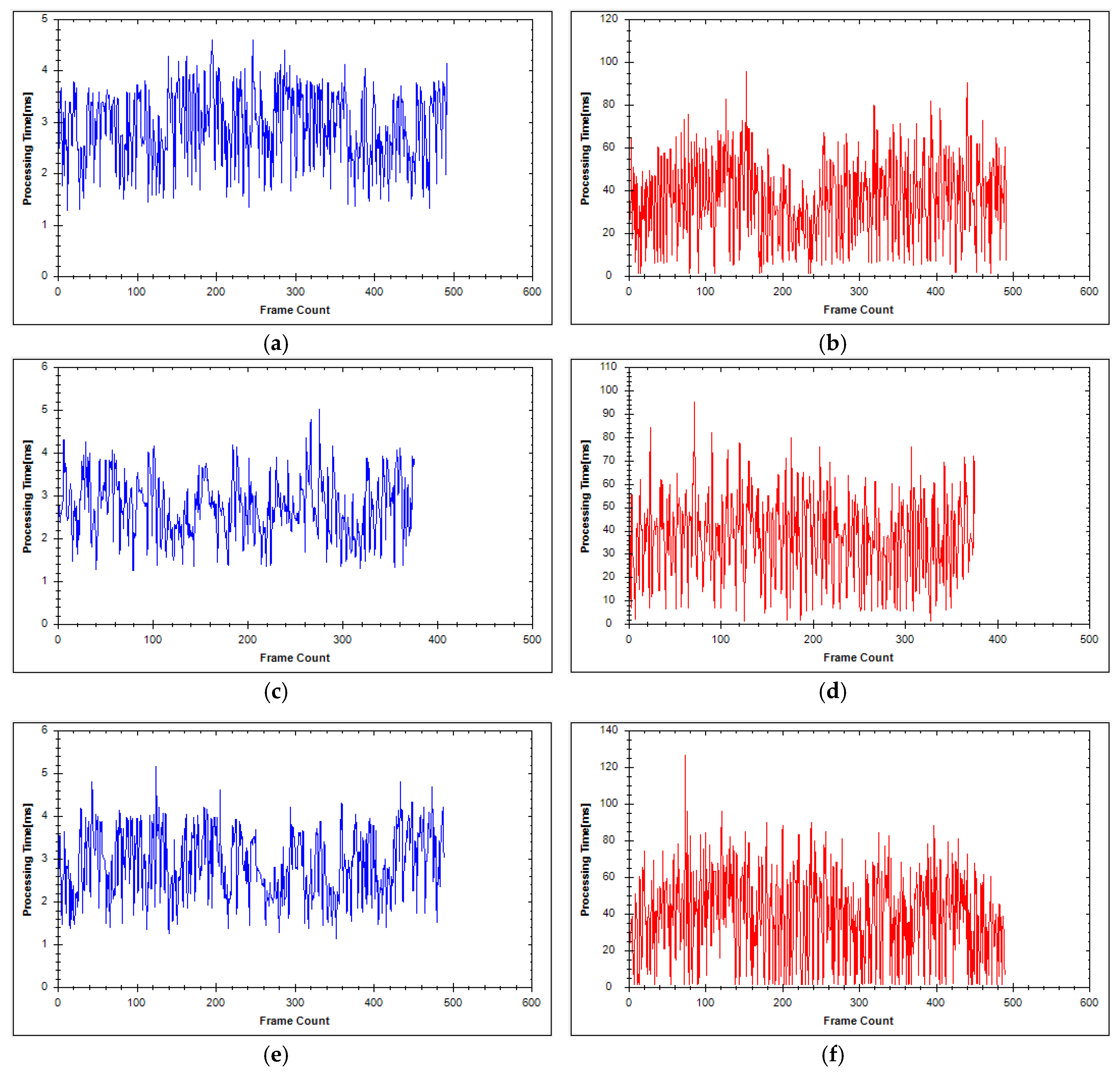
| Segmentation server 1 | 2.33 | 2.91 |
| Segmentation server 2 | 2.78 | 2.75 |
| Segmentation server 3 | 2.97 | 2.87 |
| Average Time | 2.69 | 2.84 |
| Server | Processing Time (ms) | |
|---|---|---|
| Experiment 1 | Experiment 2 | |
| Reconstruction server 1 | 31.55 | 36.14 |
| Reconstruction server 2 | 34.41 | 37.04 |
| Reconstruction server 3 | 37.74 | 39.06 |
| Average Time | 34.57 | 37.41 |
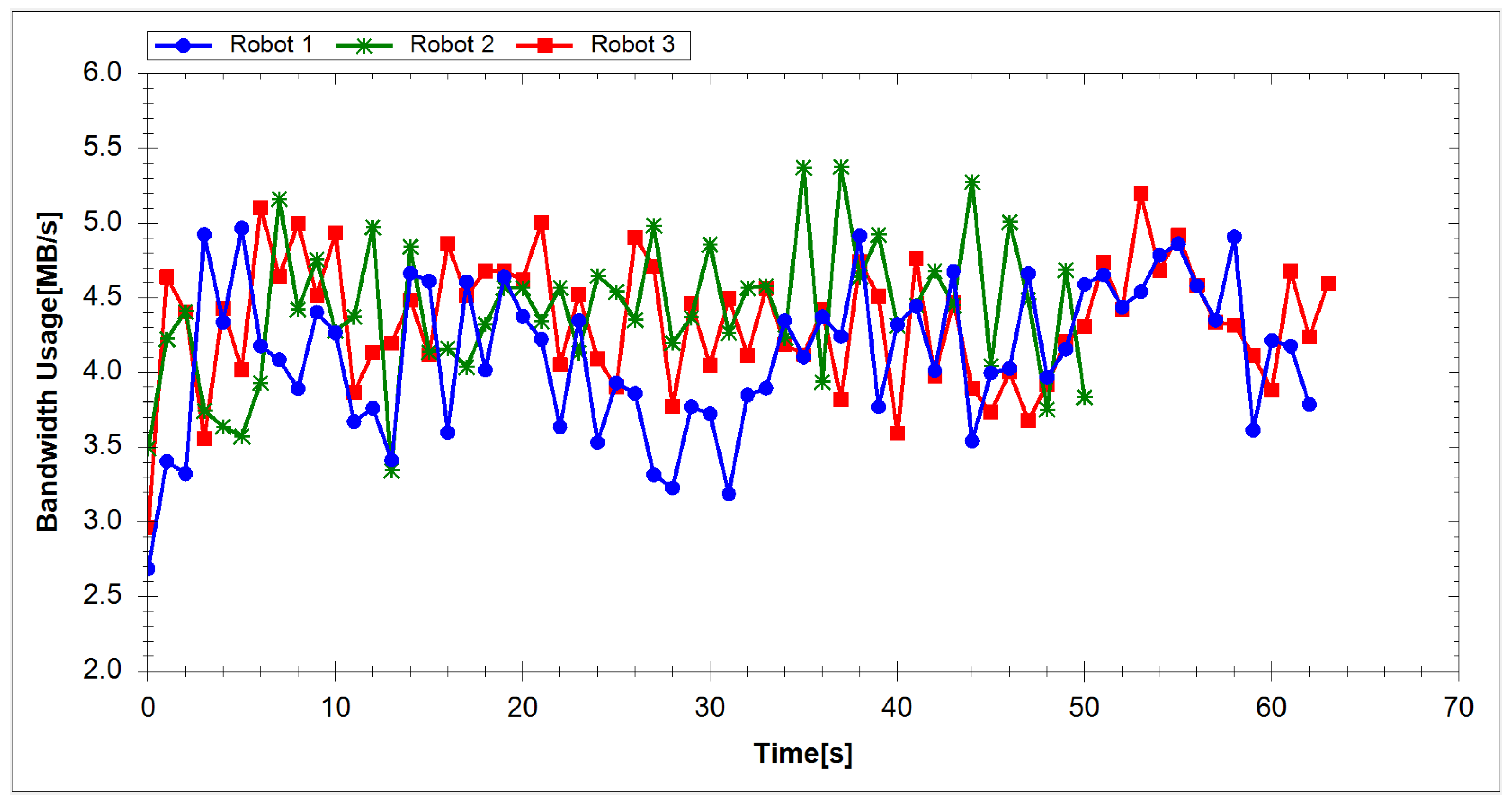
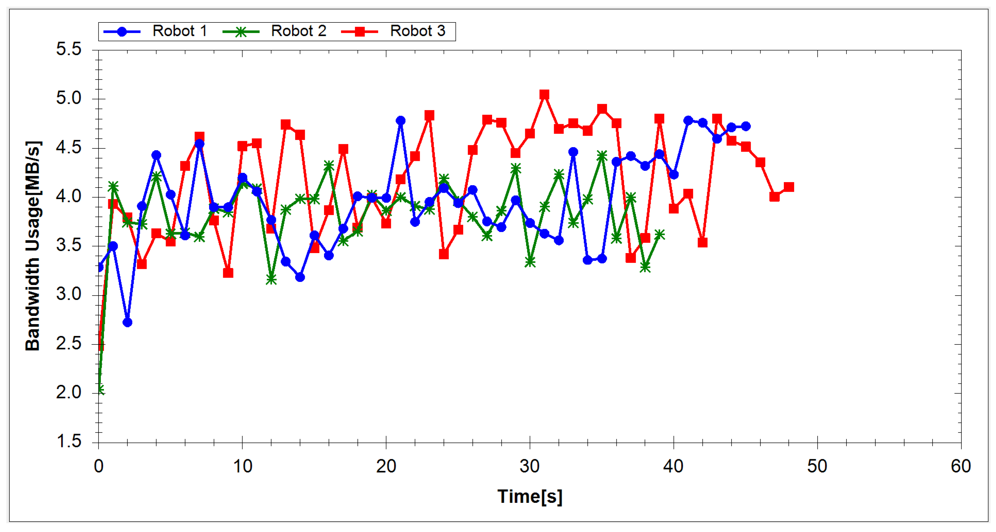
| Robot | Network Usage (MB/s) | |
|---|---|---|
| Experiment 1 | Experiment 2 | |
| Robot 1 | 4.11 | 3.97 |
| Robot 2 | 4.40 | 3.82 |
| Robot 3 | 4.34 | 4.17 |
| Average Value | 4.28 | 3.99 |
© 2017 by the author. Licensee MDPI, Basel, Switzerland. This article is an open access article distributed under the terms and conditions of the Creative Commons Attribution (CC BY) license (http://creativecommons.org/licenses/by/4.0/).
Share and Cite
Chu, P.M.; Cho, S.; Fong, S.; Park, Y.W.; Cho, K. 3D Reconstruction Framework for Multiple Remote Robots on Cloud System. Symmetry 2017, 9, 55. https://doi.org/10.3390/sym9040055
Chu PM, Cho S, Fong S, Park YW, Cho K. 3D Reconstruction Framework for Multiple Remote Robots on Cloud System. Symmetry. 2017; 9(4):55. https://doi.org/10.3390/sym9040055
Chicago/Turabian StyleChu, Phuong Minh, Seoungjae Cho, Simon Fong, Yong Woon Park, and Kyungeun Cho. 2017. "3D Reconstruction Framework for Multiple Remote Robots on Cloud System" Symmetry 9, no. 4: 55. https://doi.org/10.3390/sym9040055
APA StyleChu, P. M., Cho, S., Fong, S., Park, Y. W., & Cho, K. (2017). 3D Reconstruction Framework for Multiple Remote Robots on Cloud System. Symmetry, 9(4), 55. https://doi.org/10.3390/sym9040055