1. Motivation
Supramolecular assembly is prevalent in nature, healthcare and engineering, but poorly understood. The assembly starts with identical copies of structures drawn from a small number of types. Modeling these starting structures as rigid bunches of spheres is well suited to assembly processes driven by so-called short-range or hard sphere interaction potentials.
More formally, an input to a computational model of an assembly process is an assembly system consisting of the following:
A collection of k rigid molecular components belonging to a few types; a rigid component is specified as the set of positions of the centers of their constituent atoms, in a local coordinate system. In many cases, an atom could be the representation of the average position of a collection of atoms in an amino acid residue. Note that an assembly configuration is given by the positions and orientations of the entire set of k rigid molecular components in an assembly system, relative to one fixed component. Since each rigid molecular component has six degrees of freedom, a configuration is a point in dimensional Euclidean space.
The pairwise component of the potential energy function of the assembly system is specified as a sum of potential energy terms between pairs of constituent atoms
i and
j in two different rigid components of the assembly system. The weak interaction between the rigid molecular components is captured by this potential energy function. The pairwise potential energy terms are, in turn, specified using pairwise potential energy functions similar to so-called Lennard–Jones potentials and Morse potentials [
1]. The potential energy is a function of the distance
between
i and
j.
A non-pairwise component of the potential energy function is in the form of global potential energy terms that capture the tethers between the rigid components within a monomer, as well as other global potential energy terms that implicitly represent the solvent (water or lipid bilayer membrane) effect [
2,
3,
4]. These are independent of particular pairs of atoms.
It is important to note that all of the above potential energy terms are functions of the assembly configuration.
The formal conceptual framework we develop here is inspired by the following types of prediction questions.
Input: the 3D descriptions of the rigid molecular components and their interactions (
Section 2 describes how they are formally specified). Output: prediction of the final assembly structures and their likelihood.
Input: as in the previous item, plus a 3D configuration of the final assembled structure. Output: prediction of those interactions that are crucial for the assembly process to terminate in the given input assembly configuration.
Input: as in the previous item. Output: prediction of minimal alterations of the building blocks or interactions that would significantly increase the likelihood of the assembly process terminating in the given input assembly configuration.
Input: as in the previous item; additionally, more than one choice of final assembly configuration. Output: prediction of key events, such as specific intermediate sub-assembly configuration choices during assembly that determine which one of the final assembly configurations is more likely to result.
Experimentally, in vitro or vivo, these types of predictions about supramolecular assembly processes are difficult because of the remarkable rapidity, spontaneity and robustness of assembly processes. The prediction tasks highlight combinatorial explosion and, thus, the insufficiency of experimentation (trying various possibilities) and guesswork, even with the help of known data on similar assemblies and biological knowledge about evolutionarily-conserved structures. In addition, many of the current experimental methods are labor and resource intensive, making blind alleys expensive in time and effort.
On the other hand, computer simulations guided by theoretical first principles and standard paradigms, such as Monte Carlo (MC) or molecular dynamics (MD), are limited due to the reasons detailed in the next subsections.
1.1. Assembly Configurational Volume
The stability and binding affinity of subassemblies depend on free energy, whose landscape in the case of assembly is heavily influenced by configurational entropy (volume measure of microstates corresponding to a macrostate; see [
5]); this depends on accurate computation of configurational volumes by sampling, attempted by a long and distinguished series of methods [
5,
6,
7,
8,
9,
10,
11,
12,
13]. Assembly configuration spaces are high dimensional, and the number of required samples is typically exponential in the dimension. Sampling on a high-dimensional ambient space grid typically means computing a large proportion of samples that lie outside any region of interest, which is effectively of lower dimension, and these samples must be discarded. Not only are the relevant regions in the case of short-ranged potentials of effectively lower dimension, they are also geometrically/topologically complex; hence, grid-based sampling in Cartesian space, as well as non-ergodic methods, like MC or MD, have to generate impractically dense sampling to accurately reflect the volume/measure ratios of these important, relatively low volume regions having complex geometry and topology. These methods do not exploit the abundance of symmetries of the landscape. They are used both for assembly processes, whose feasible regions are defined by one-sided pairwise distance equalities and inequalities between atom-centers, and folding processes, where the feasible regions are defined by pairwise distance equalities. The difference of complexity between the two is a litmus test for the limitations that are addressed by the Cayley configuration space approach taken by efficient atlasing and search of assembly landscapes (EASAL) described in
Section 1.5.
Conventional methods to compute the energy landscape of small clusters are based on searching for local minima [
1,
14,
15]. Point group symmetrization schemes [
16,
17,
18] and local rigidification schemes [
19,
20] have been exploited in global optimization algorithms to gain computational efficiency.
Because of the complexity of the problem of dealing with the short range of interaction of hard spheres leading to narrow regions of lower potential energy, separated by vast flat parts, conventional local minima-based methods for energy landscape computation [
14] are limited. These methods have the additional disadvantage of small perturbations to energy values requiring complete recomputation, and also, they do not deal well with the very flat landscape that is the signature of short-range potentials.
An alternative approach for short-range potentials is to consider the “sticky sphere limit” based on taking the limit as the range of interaction goes to zero [
21,
22,
23]. In this limit, the energy landscape reduces to a collection of manifolds of different dimensions, glued together at their boundaries (formally, a Thom–Whitney stratification of real semi-algebraic sets), as described in theoretical models proposed independently and separately by Holmes-Cerfon
et al. [
24] in 2013 and by the first author’s research group [
25,
26] in 2011.
The background provided in the remainder of this section recalls previously-developed concepts for describing assembly configuration spaces. This motivates the conceptual framework for symmetry in assembly under short-range potentials given in
Section 2.
1.2. Kinetics, Topology and Geometric Complexity
Kinetics and transition rates between subassemblies also require an explicit understanding of the geometry, topology and multiple paths in the assembly configuration space. For cluster assemblies from spheres, there are a number of methods [
27,
28,
29,
30,
31,
32,
33] to compute the entire configuration space of small molecules, such as cyclo-octane [
34,
35,
36]. Some methods from robotics and computational geometry [
12], such as the probabilistic roadmap [
37], effectively give bounds to approximate free energy without relying on MC or MD sampling. Starting from MC and MD samples, recent heuristic methods infer topology [
38,
39,
40,
41] and use topology to guide dimensionality reduction [
42]. Yet, most prevailing methods are unable to extract the topology in a sufficiently efficient and accurate manner as to be able to feasibly compute volume or path integrals (required for entropy or kinetics computations), even for small assemblies. Moreover, even those prevailing methods that exploit symmetry in the configuration space to compute free energy and kinetics do not employ a formal and precise group-theoretic framework.
1.3. Recursive Decomposition, Assembly Trees and Combinatorial Entropy
For larger, microscale assemblies, a direct study of the free energy and configurational entropy is computationally emphatically intractable. At these coarser scales, the primitives are stable subassemblies and transition rates (obtained from the computational tasks of the previous two subsections). Still, the combinatorial entropy of multiple pathways makes it difficult to isolate crucial combinations of assembly-driving interface interactions.
This issue has been addressed by the first author’s previous work on recursive decompositions [
43,
44,
45] of larger assemblies into smaller subassemblies. This work introduces structures called assembly trees and the notion of combinatorial entropy, applied to model viral capsid assembly in [
46].
While trees of various types have been used to model various processes related to assembly [
47,
48], to the best of our knowledge, the assembly trees from [
46] have a formal structure that is distinct from other tree representations of assembly pathways. In particular, non-root nodes of the assembly tree contain subassemblies, rather than configurations of the entire assembly system; and any pair of nodes that are incomparable (neither ancestor or child in the tree) is a disjoint sub-assembly,
i.e, they do not contain any common rigid components; moreover, only rigid sub-assembly configurations are represented. In addition, the authors have taken the first steps towards precisely formalizing the effect of symmetries on a highly simplified version of assembly trees; specifically, their orbits under the action of a fixed group of symmetries, called assembly pathways [
49]. These concepts will be discussed in detail in
Section 2 and
Section 3.
1.4. Symmetry in Chemistry
Since spheres within rigid bunches of an assembly system could be identical and bunches could be identical, as well, the underlying symmetry groups could be of large order, which grow with the number of participating spheres and bunches. Therefore, all of the tasks in the previous three subsections can be significantly simplified by taking advantage of natural symmetries of the configuration space that arise due to identical assembling units, their symmetries and symmetries of the final assembled structure. However, none of the prevailing methods discussed above computationally incorporates these symmetries. Group theory has been used to study the symmetry of molecules and molecular orbits [
50,
51,
52,
53] for a long time. The well-known Pólya enumeration theorem [
54], which provides a method to find the number of orbits of a group action, is motivated by the problem of enumerating permutational isomers of a given molecular skeleton. Group theory is widely used in crystallography to describe crystallographic symmetry and to classify crystal structures [
55,
56]. Other applications include using the molecule symmetry group in studying molecular spectroscopy [
57] and using generating functions in understanding nuclear spin statistics of nonrigid molecules [
58]. However, most of these works only involve the symmetry of individual structures. The literature is sparse in the context of symmetry in assembly systems or in configuration spaces.
1.5. EASAL: Efficient Atlasing and Search of Assembly Landscapes
A recent method of the first author, EASAL (efficient atlasing and search of assembly landscapes) [
25,
26], formally addresses the issues highlighted in the first two subsections above: computation of configurational entropy and kinetics, via geometrization, stratification and convexification using Cayley parameterization of assembly configuration spaces. Geometrization and stratification were also used later in [
24] independently (as mentioned at the end of
Section 1.1): the geometrization is achieved in [
24] via a somewhat different process consistent with smooth potential energy functions, while the stratification is the standard Thom–Whitney stratification of semi-algebraic sets as laid out in [
25,
26].
On the other hand, Cayley convexification based on [
59] is a unique feature of EASAL not present in [
24], which makes it tractable to sample and compute entropy integrals over higher dimensional constant potential energy regions of the assembly configuration space. In addition, Cayley convexification helps formalize and precisely explain the intuitively clear observation that assembly configuration spaces are significantly simpler geometrically and topologically than folding configuration spaces. The difference in complexity is especially stark when there are cycles of pairwise constraints between atom centers.
We describe the geometrization and stratification aspects of EASAL’s approach below. Stratification is explained in further detail in
Section 2, and Cayley parameters for configuration spaces and convexification based on [
59] are explained in
Section 4.
1.5.1. Geometrization
The assembly configuration space is represented as a semi-algebraic set satisfying geometric constraints specified as distance inequalities between atom centers. The short-range or hard sphere potential interaction is typically discretized to take different constant values on three intervals for the distance value : , and Typically, , the so-called van der Waals or steric radius, specifies “forbidden” regions around atoms i and Additionally, is a distance where the attractive (electrostatic or other weak) forces between the two atoms are no longer strong (typically, these forces decay as the reciprocal of some power of the distance between atom centers). Intuitively, the interval is where the repulsive force highly dominates, and is where the attractive force and repulsive forces are balanced; also, is where neither force is strong. Over these three intervals, respectively, the potential assumes a very high value, a very low value and a medium value All of these bounds for the intervals for , as well as the values for the potential on these intervals are specified as part of the input to the assembly model. These constants are specified for each pair of atoms i and j, i.e., the subscripts are necessary. The interval with the low value is called the well. The hard sphere potentials are defined solely by the van der Waals’ forbidden distance constraint, .
The information in the potential energy landscape can thus be geometrized, i.e., represented using assembly constraints, in the form of distance intervals. These constraints define feasible configurations. The set of feasible configurations is called the assembly configuration space. The active constraint regions of the configuration space are regions where at least one of the short-range inter-atom distances lies in the potential energy well, i.e., the interval .
1.5.2. Stratification
The above geometrization of an assembly configuration space makes it natural to stratify an assembly configuration space into an atlas of active constraint regions. More details are provided in
Section 2.4. The active constraint regions of the configuration space are regions where at least one of the inter-atom distances lies in the potential energy well. The active constraint regions are stratified by dimension into a topological Thom–Whitney complex, with the boundary region being one dimension smaller. The active constraint regions can be modeled as so-called convexifiable Cayley configuration spaces [
59], a combinatorially-definable concept by first labeling each region by its unique active constraint graph (see
Section 2). A demo movie of EASAL is available at [
60]. Standard algorithms can be employed for a fast computation of paths from one configuration to another in the atlas. However, the computation of entropy integrals over these paths poses several challenges.
1.6. Organization and Contribution
This is a primarily expository paper that develops a novel, original framework for dealing with symmetries in configuration spaces of assembling spheres under short-range potentials. It is motivated by a longer term goal to exploit natural symmetries using assembly trees and other concepts described in the previous sections that have appeared in various avatars in the community, including our work on EASAL. Such an understanding of symmetries is essential for significantly reducing the complexity of the computation of configurational and combinatorial entropy, as well as kinetics, since spheres within rigid bunches of an assembly system could be identical and bunches could be identical, as well, giving underlying symmetry groups of large order, which grow with the number of participating spheres and bunches.
To this end, we develop a formal conceptual framework for assembly under short-range potentials, as an assembly of rigid bunches of spheres. As different definitions of assembly macrostates are appropriate in different contexts, for example depending on whether different copies of identical atoms or molecules are considered interchangeable or not, we carefully define and differentiate between the congruence and isomorphism of configurations. We then show how symmetries of assembly configuration spaces arise due to: multiple copies of identical building blocks (in particular, when these building blocks are rigid bunches of spheres), internal symmetries of building blocks and the symmetries of the final assembled structure.
The organization of this paper is as follows. In
Section 2, we define the new conceptual framework for symmetry in assembly under short-range potentials (or an assembly of rigid bunches of spheres) leading to the main Theorem 4. An application of some of these results on symmetry can be found in [
26]. In
Section 3, we illustrate one aspect of our approach [
49] for computing combinatorial entropy using generating functions for counting the number and size of simplified assembly pathways (orbits of a symmetry group action on assembly trees). Note that while this simple example has a fixed group size, the method demonstrated applies also when the underlying symmetry group grows with the size of the system. In
Section 4, open questions and directions are given.
2. Framework for Symmetry in an Assembly
In this section, we define natural groups of symmetries acting on various previously-defined objects related to symmetry that are described in
Section 1 and later in this section. The four new groups we defined are the weak automorphism group, the strict congruence group, the strict order preserving isomorphism group and the strict permuted congruence group of an assembly configuration. We consider the action of these groups on various objects defined in previous literature on assembly and sketched in
Section 1 [
25,
26,
46], such as assembly configuration space, active constraint regions, active constraint graphs, assembly paths and trees. These resulting symmetry classes will be used to formalize the main new Theorem 4 and two applications in Example 1 and
Section 3, as well as open problems in the last section of this paper.
Let X be a set under the action of a group G, and x be any element of X. The orbit of x under G is the set . An element g of G fixes x if . The stabilizer subgroup of x in G is the group of all elements in G that fix x, i.e., .
The following theorem from standard group theory can be used to determine the number of orbits and the size of orbits for various objects defined in this section. An explicit application of this theorem is shown in the next section.
Theorem 1. Let X be a set under the action of a group G. For all ,
the equalities:andhold, where is the number of orbits of X and is the set .
Different definitions of macrostates are appropriate in different contexts, for example depending on whether different copies of identical atoms or molecules are considered interchangeable or not. For this reason, we carefully define and differentiate between the congruence and isomorphism of configurations.
In order to give a physically meaningful formalization of an assembly system under short-range potentials, we define the notion of a bunch, i.e., a rigid configuration of spheres of varying colors and radii.
2.1. A Bunch and Its Symmetries
Let denote the group of orientation-preserving isometries of .
A bunch is a tuple where is an ordered set of points in , and are functions defining colored spheres centered at the points in P. Specifically, where C is a finite set of “colors”, and , such that the spheres are non-intersecting, i.e., for any . The map δ is interpreted as the width of the annulus specified by the potential energy well and is used in the definition of an active constraint graph of an assembly configuration later in this section. For a bunch B, is used to denote the point set B; similarly, we have and .
Two bunches
and
are
isomorphic if there is an element
ϕ of
and a permutation
, such that
for all
i, where
, and
ϕ preserves the color, radius and annulus of points. In this case, with a slight abuse of notation, we write
, where
denotes the set of bunches that are isomorphic to
B under
ϕ and some permutation in
. See
Figure 1 for an example.
Two bunches and are strictly isomorphic, if there is a permutation such that B and are isomorphic under π and the identity element in . The weak automorphism group of B, denoted , is the group of all permutations that take B to a strictly isomorphic .
Figure 1.
Two isomorphic bunches of five spheres.
Figure 1.
Two isomorphic bunches of five spheres.
Two bunches and are order-preserving isomorphic or congruent, if there is a , such that B and are isomorphic under ϕ and the identity permutation. In this case, with a slight abuse of notation, we write .
We have the following observation that describes strict isomorphism using the notion of congruence.
Observation 2. Two congruent bunches B and are strictly isomorphic, if and only if , where and denote the unordered point sets of B and , respectively, and for all , , , .
2.2. An Assembly Configuration Space and Its Symmetries
An
assembly configuration is an ordered set
, where
is a bunch for all
i, such that for all
and all
, we have:
Two assembly configurations
and
are configurations of the same assembly system (see
Section 1) if
is congruent to
for some permutation
, for all
i. Notice that the congruence between bunches could be different for each
i. The set of all assembly configurations of an assembly system is called an
assembly configuration space. The assembly configuration space containing the assembly configuration
is denoted
or simply
when the context is clear.
In the following discussion, we always restrict our universe to assembly configurations in the same assembly configuration space.
Two assembly configurations and are isomorphic if there is an element ϕ of (isomorphism between bunches) and a permutation , such that for all i, is isomorphic to under ϕ and a permutation , where .
Two assembly configurations and are strictly isomorphic, if there is a permutation , such that for all i, is isomorphic to under the identity element in and a permutation , where . Thus, a strict isomorphism is a tuple of permutations , where and . The weak automorphism group of , denoted , is the group of all such tuples that take to a strictly isomorphic , with the group operation .
Note that all assembly configurations in the same assembly configuration space have the same weak automorphism group. Thus, we define the weak automorphism group of an assembly configuration space , denoted , to be the weak automorphism group of any assembly configuration in .
Two assembly configurations and are congruent if there is an isomorphism that preserves both the order of the bunches and the order of points within each bunch, i.e., for all i, is congruent to under ϕ. Two assembly configurations and are strictly congruent if they are both congruent and strictly isomorphic. In general, we think of two strict congruent assembly configurations as the same. The strict congruence group of an assembly configuration is the stabilizer of the set strictly congruent assembly configurations of under . It is the stabilizer subgroup of the assembly configuration under .
Two assembly configurations and are order-preserving isomorphic if there is an isomorphism that preserves the order of the bunches, i.e., for all i, is congruent to . Two assembly configurations and are strictly order preserving isomorphic if they are both order-preserving isomorphic and strictly isomorphic. The strict order-preserving isomorphism group of an assembly configuration is the stabilizer of the set of strictly order-preserving isomorphic configurations of under .
Two assembly configurations and are permuted congruent if there is an isomorphism that preserves the order of points within each bunch, i.e., there is an element ϕ of and a permutation , such that for all i, is congruent to under ϕ. Two assembly configurations and are strictly permuted congruent if they are both permuted congruent and strictly isomorphic. The strict permuted congruence group of an assembly configuration is the stabilizer of the set of permuted congruent configurations of under .
For an example, refer to
Figure 2. The assembly configuration
consists of three congruent bunches. The assembly configuration
is obtained from
with a strict congruence
induced by a rotation in
, where
, and
for all
i. The assembly configuration
is obtained from
with a strict permuted congruence
, where
σ is a cyclic permutation of the three bunches, and
for all
i. On the other hand,
is obtained from
with a strict isomorphism
, where
σ is a cyclic permutation of the three bunches,
and
.
Figure 2.
The assembly configuration consists of three isomorphic bunches. is obtained from with a strict congruence; is obtained from with a strict permuted congruence; and is obtained from with a strict isomorphism that is neither a strict congruence, nor a strict permuted congruence, nor a strict order preserving isomorphism.
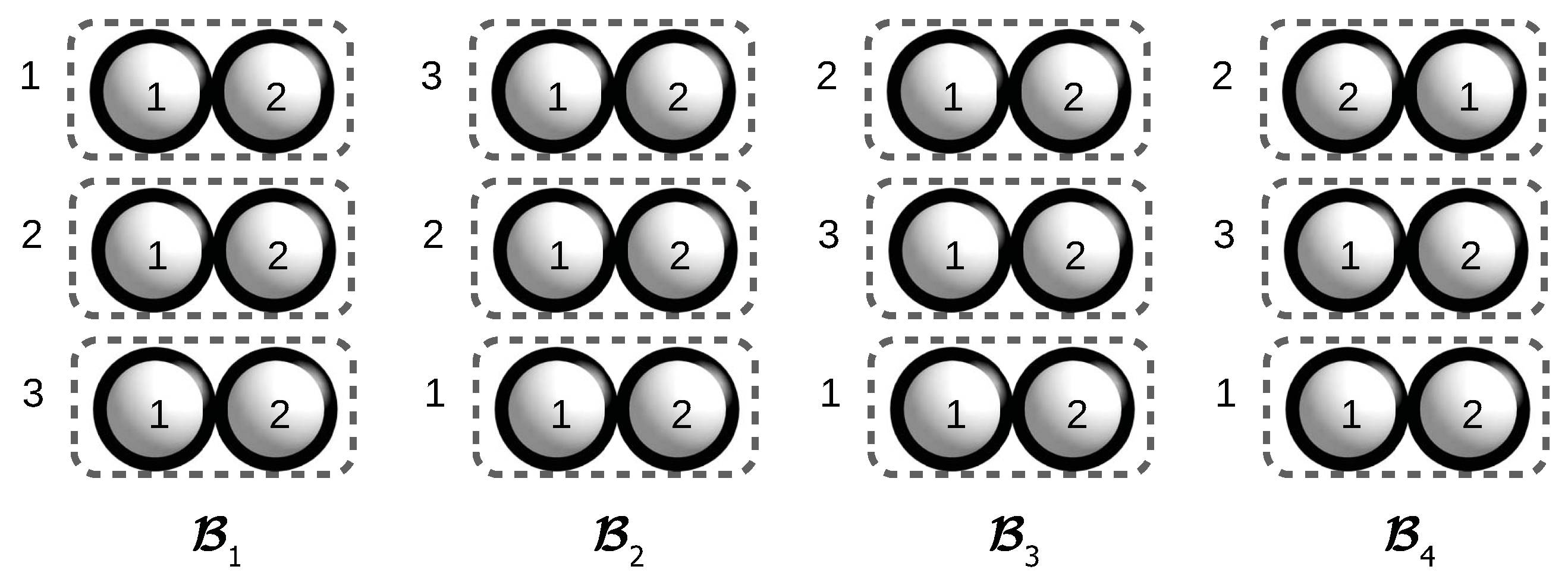
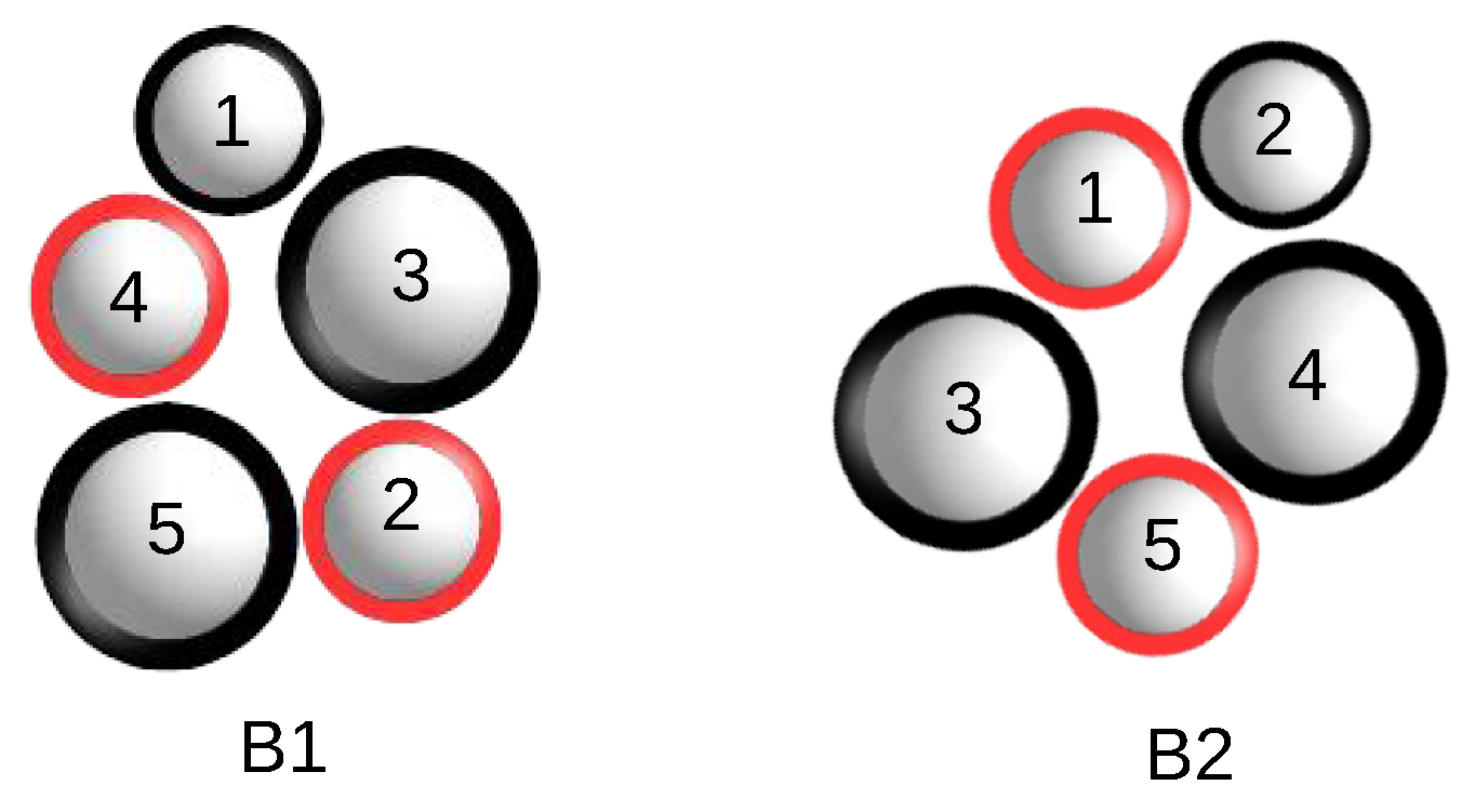
Figure 3 shows another example of four assembly configurations each containing two bunches. The strict congruence group
of the assembly configuration
is of size two and contains those tuples
, where
,
,
. The weak automorphism group
of the assembly system is of size four and contains those tuples
, where
,
,
. All four strictly isomorphic assembly configurations are obtained by applying
to the assembly configuration
. Notice that
and
(
and
) are strictly congruent, while
and
are strictly order-preserving isomorphic. The orbit of
under
is of size two and consists of
and
.
Figure 3.
Four assembly configurations obtained by applying on the assembly configuration . is obtained from with a congruence, while is obtained from with a strict order-preserving isomorphism.
Figure 3.
Four assembly configurations obtained by applying on the assembly configuration . is obtained from with a congruence, while is obtained from with a strict order-preserving isomorphism.
We have the following observations for alternative characterizations of strict congruence, strict order-preserving isomorphism and strict permuted congruence of assembly configurations.
Observation 3. Given two assembly configurations and in the same assembly configuration space, and
are strictly congruent if and only if they are congruent, and- (*)
and have the same unordered partition of the unordered point set into bunches, i.e., , where is the unordered point set of the bunch , and each point has the same color, radius and annulus in and .
and are strictly order-preserving isomorphic if and only if they are order preserving isomorphic and satisfy the condition (*).
and are strictly permuted congruent if and only if they are permuted congruent and satisfy the condition (*).
2.3. Symmetries in an Active Constraint Graph and an Active Constraint Region
An
active constraint graph of an assembly configuration
is a graph
, where the vertex set
V has one vertex for each point
, labeled by a tuple
, representing that the point
p appears as the
i-th point
in the
l-th bunch
of
, and a vertex pair
if
x and
y lie in distinct bunches of
and:
An element of the weak automorphism group of ’s assembly configuration space acts on by taking the tuple to .
Two active constraint graphs are isomorphic if there is a , such that . In this case, we say or .
The automorphism group of an active constraint graph G is the group of elements , such that , i.e., it is the stabilizer subgroup .
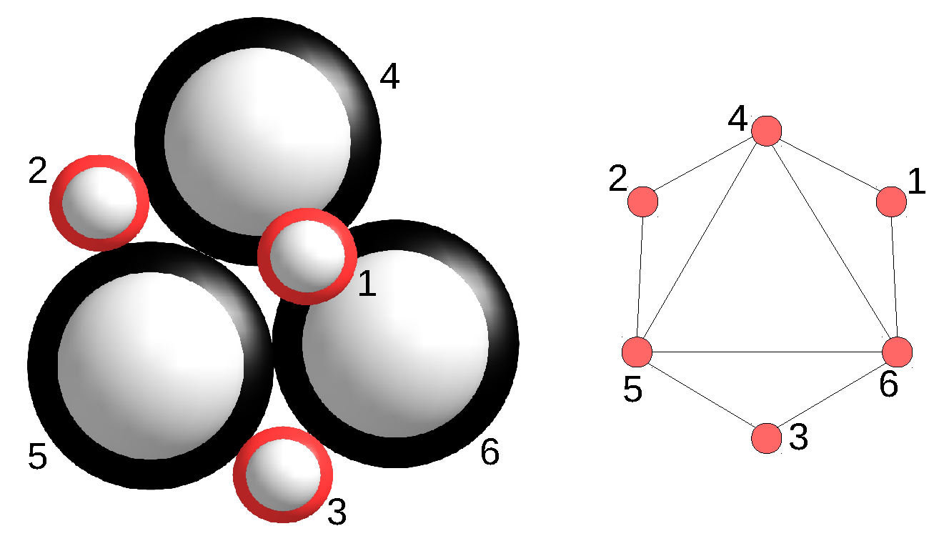
For example,
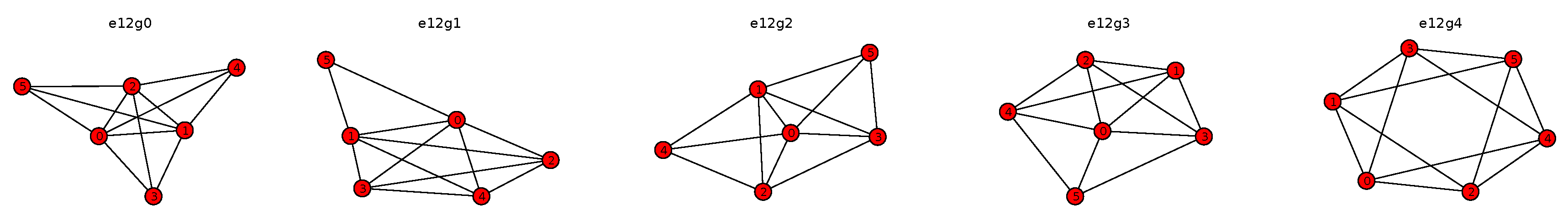
Figure 4 shows all of the non-isomorphic active constraint graphs with 12 edges of an assembly system consisting of six bunches, where all bunches are identical singleton spheres.
Figure 4.
All non-isomorphic active constraint graphs with 12 edges of an assembly system of six bunches that are identical singleton spheres. The label on top is automatically generated by EASAL and specifies the orbit number of the shown active constraint graph.
Figure 4.
All non-isomorphic active constraint graphs with 12 edges of an assembly system of six bunches that are identical singleton spheres. The label on top is automatically generated by EASAL and specifies the orbit number of the shown active constraint graph.
Note: It is clear that
. Moreover, there are assembly configurations
, such that
,
i.e., the strict congruence group of
does not have all of the automorphisms of the corresponding active constraint graph. Refer to the assembly configuration
and its active constraint graph
G in
Figure 5, where each bunch is a singleton sphere. The permutation
is contained in
. However, it is not contained in the strict congruence group
of the assembly configuration.
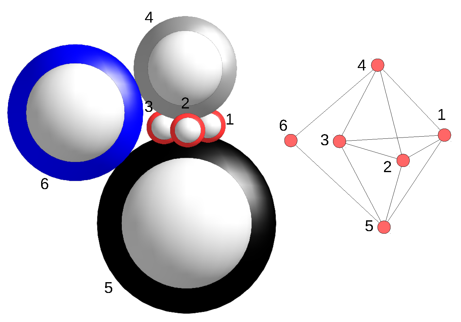
Figure 5.
An assembly configuration whose automorphism group is strictly contained in that of the corresponding active constraint graph. Here, the bunches are singleton spheres, and bunches of the same color have the same , r and δ.
Figure 5.
An assembly configuration whose automorphism group is strictly contained in that of the corresponding active constraint graph. Here, the bunches are singleton spheres, and bunches of the same color have the same , r and δ.
The full graph of an active constraint graph G is obtained by adding edges to G to make the set of vertices in each bunch into a clique.
An active constraint region of the assembly configuration space contains all assembly configurations with the active constraint graph . The action of elements of on an active constraint region and the stabilizer of an active constraint region in are well-defined by the action of on assembly configurations.
The following theorem gives containment and equality relations between stabilizer subgroups of an active constraint graph, an active constraint region and individual configurations in the active constraint region.
Theorem 4. For an active constraint graph of an assembly configuration space ,
it holds that:In addition, there exist active constraint graphs G of assembly configuration spaces where the above containment is strict, i.e., Proof. (1) It is straightforward to see that
. We give an example to show the existence of
G where
for any assembly configuration
of
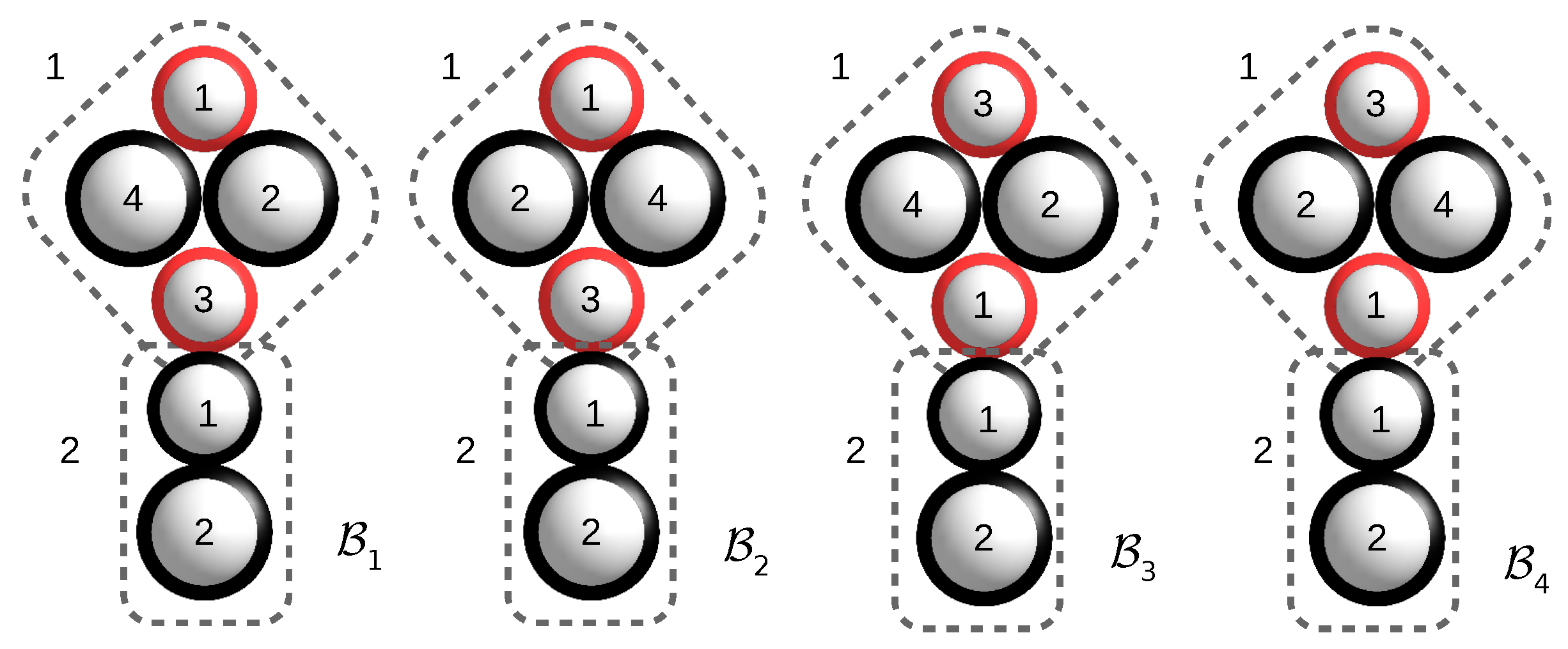
G. Refer to the assembly configuration in
Figure 6, where each bunch is a singleton sphere. The permutation
is contained in the automorphism group
of the active constraint graph
G. However, it is not contained in the strict congruence group of any corresponding assembly configuration, as the position of the sphere six is asymmetric with respect to
in any assembly configuration of
G. Thus,
for any assembly configuration
of
G.
Figure 6.
Any assembly configuration corresponding to the active constraint graph G has its strict congruence group strictly contained in . Here, the bunches are singleton spheres, and bunches of the same color have the same , r and δ.
Figure 6.
Any assembly configuration corresponding to the active constraint graph G has its strict congruence group strictly contained in . Here, the bunches are singleton spheres, and bunches of the same color have the same , r and δ.
(2) : from the definition of permutations in the weak automorphism group of the assembly configuration space, it follows that . To show , consider any element . For any assembly configuration , if a pair of spheres are “touching” (i.e., they yield an edge in the corresponding active constraint graph), it must be the case that are also “touching” in , since . Similarly, ψ must map “non-touching” pairs to “non-touching” pairs. Therefore, . ☐
Remark 1. We expect the strict order-preserving isomorphism group and the strict permuted congruence group of an assembly configuration to lie between the strict congruence group and the automorphism group of its active constraint graph. However, the containment relationship between these two groups is not clear.
2.4. Symmetries in Stratification, Assembly Path and Pathway
A stratification of the assembly configuration space is a partition of the space into strata of that form a filtration , . Each is a union of active constraint regions , where the corresponding active constraint graph G has independent edges, i.e., inequality constraints are active. Each active constraint graph G is itself part of at least one, and possibly many, hence, l-indexed, nested chains of the form .
These induce corresponding reverse nested chains of active constraint regions
:
. Note that here, for all
,
is closed and
j dimensional. See
Figure 7 for an example of assembly configuration space stratification.
Given two active constraint graphs and , (resp. ) is a parent of (resp. ) (resp. is a child of ) if , and there does not exist an active constraint graph , such that . The parent-child relation provides a Hasse diagram of active constraint regions in the stratification of .
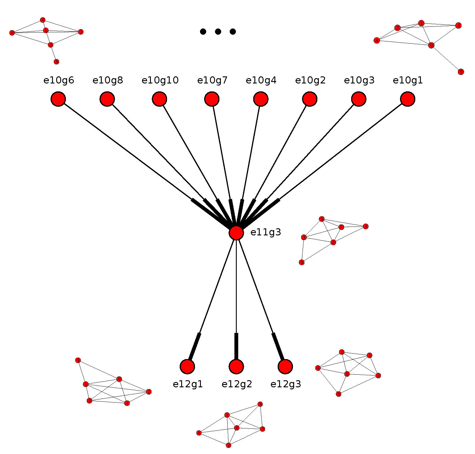
Figure 7.
A fundamental region of the stratification for the assembly configuration space of the assembly configurations in
Figure 4 of six bunches, with each bunch being a singleton sphere and all bunches identical. Therefore,
is the complete symmetric group of the permutations of six elements,
. Each node shown is an orbit representative of an active constraint region corresponding to an active constraint graph. The grey part is those active constraint graphs (orbit representatives) whose corresponding constraint regions are empty. The example active constraint graph representatives on the right have arrows pointing to their regions in the stratification. The labels in the circles are unimportant: they are automatically generated and specify an orbit of an active constraint graph (example shown on the right).
An
assembly path from
to
in the stratification is a sequence
where
is a child of
for all
. A
coarse assembly path from
to
in the stratification is a sequence
where
has exactly one new rigid component
S not in
, with
S containing a set of two or more rigid components
of
. In addition, for all proper subsets
with
, the subgraphs of
induced by
Q are not rigid (The rigid components of a graph are the maximal rigid subgraphs. Two rigid components cannot intersect on more than two vertices. We refer the reader to combinatorial rigidity concepts in [
61]).
For example, In
Figure 7, the sequence of active constraint graphs on the right form an assembly path.
An
assembly forest corresponding to a coarse assembly path from
to
is the unique forest where the leaves are the maximal rigid components of
. The internal nodes are the new rigid components
S occurring in some
in the path. The children of
S are the set of rigid components
contained in
S that occur in
. The roots of the forest are the rigid components of
. An
assembly tree is an assembly forest with only one root. See
Section 3 for examples of assembly trees [
46,
49,
62].
A full (coarse) assembly path is an (coarse) assembly path from to , where is the empty active constraint graph, and is a rigid active constraint graph. A (coarse) assembly path from primitives has the first property of the full assembly path, i.e., is the empty active constraint graph, but not the last property, i.e., can be any active constraint graph. The full assembly tree and assembly tree from primitives are also defined in this way.
A path between full active constraint graphs G and H where and is a sequence , where any pair and is on some assembly path, and if k is even, if k is odd.
The fundamental domain of the stratification is the minimal sub-stratification , such that , where π acts on via its action on the active constraint regions (resp. active constraint graphs) of . In other words the active constraint regions (resp. active constraint graphs) in are orbit representatives of active constraint regions (resp. active constraint graphs) under .
An assembly pathway is an orbit of an assembly tree under . The definition extends to full and coarse assembly trees.
2.5. Example Illustrating the above Symmetries
Some of the symmetry concepts defined here were used in [
26] to efficiently compute path and higher dimensional region intervals in sphere-based assembly configuration spaces more efficiently reproducing and extending the results in [
24]. We give a brief description here in the form of an example:
Example 1. As an example,
Figure 7 shows the Hasse diagram of the fundamental region of a stratification of an assembly system of six bunches that are identical singleton spheres considered first in [
24].
Figure 8 shows an (orbit representative of an) active constraint graph of the system together with its parents and children in the Hasse diagram.
Figure 8.
The neighbors of one active constraint graph in the Hasse diagram of the stratification for the assembly system in
Figure 4.
Figure 8.
The neighbors of one active constraint graph in the Hasse diagram of the stratification for the assembly system in
Figure 4.
In addition, orbit representatives of paths help with improving the efficiency of path integrals. In
Figure 7, any path that goes down from the top of the diagram to the bottom is the orbit representative of an assembly path. In
Figure 8, the sequence
is the orbit representative of an assembly path, but not a coarse assembly path, as none of
’s rigid components contains two or more rigid components of
. On the other hand, the sequence
is the orbit representative of a coarse assembly path.
3. Enumerating Simple Assembly Pathways
In this section, we consider the action of the strict congruence group of a single final configuration on its assembly trees and use generating functions to count the number and sizes of simplified assembly pathways [
49]. Note that our approach could potentially be applied for all other groups defined in
Section 2, the largest of which is the weak automorphism group of the final configuration, which would be the same as the weak automorphism group of the assembly configuration space.
A simple assembly is modeled by a rooted tree; the leaves are abstract representation of individual bunches, the root representing the final assembled configuration. The internal vertices represent intermediate stages of assembly, simplified to be subsets instead of subgraphs of the root. This simplification results in a loss of information about the assembly configuration space and active constraint graphs of the intermediate stages of assembly. To compensate, the group is taken to be the automorphism group G of the graph of the assembled structure at the root instead of the weak automorphism group of the assembly configuration space.
The definitions of assembly trees and pathways are simplified as follows. Given a finite group
G acting on a finite set
X, we will define a simplified assembly pathway for the pair
. First, a
simplified assembly tree is a rooted tree for which each internal vertex has at least two children and whose leaves are bijectively labeled with elements of a set
X. There is an induced labeling on all of the vertices of a simplified assembly tree by labeling a vertex
v by the set of labels on the leaves that are descendents of
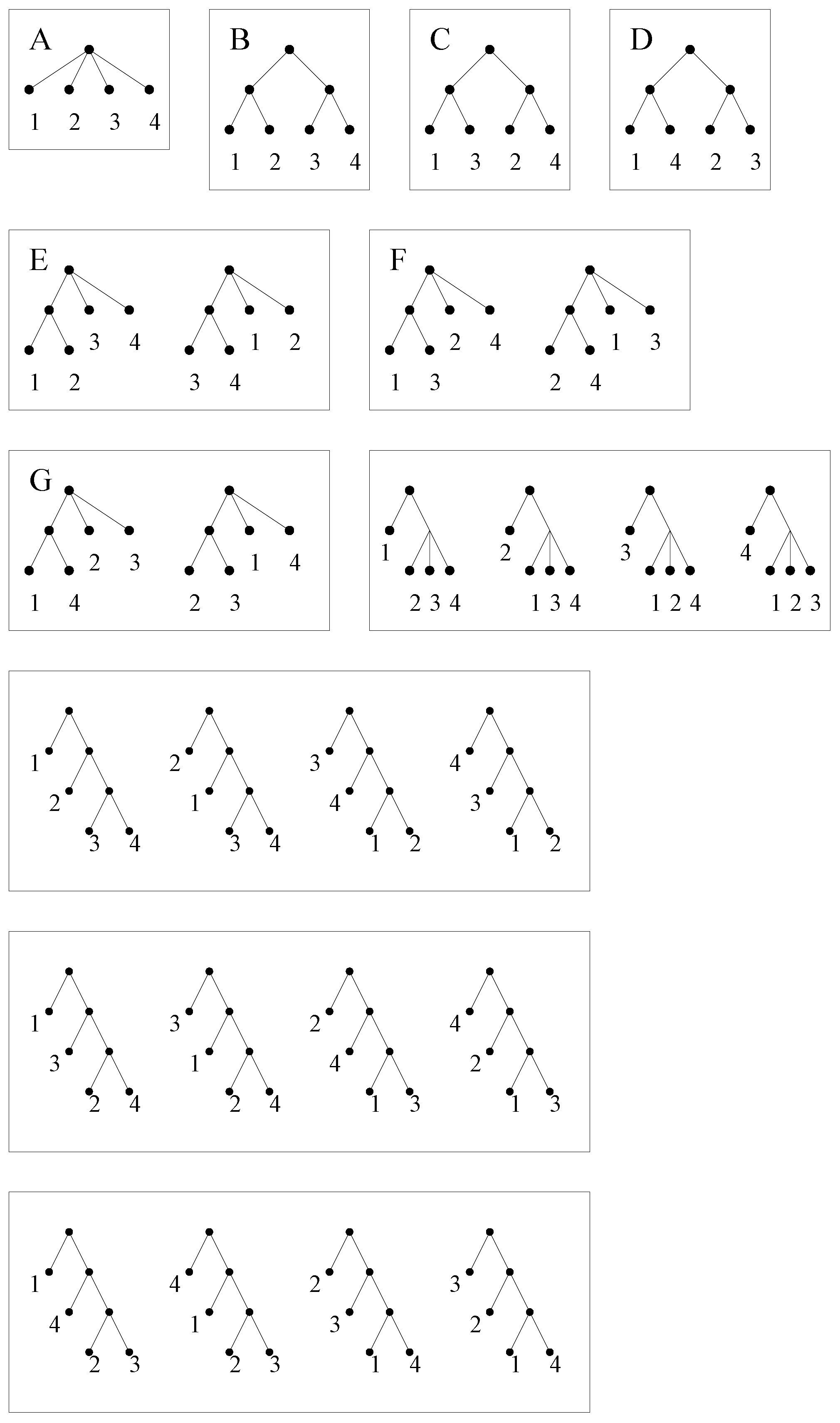
v. We identify each vertex of a simplified assembly tree with its label. Two simplified assembly trees are considered identical if there is a root-preserving, adjacency-preserving and label-preserving bijection between their vertex sets. The 26 simplified assembly trees with four leaves, labeled in the set
, are shown in
Figure 9.
For a simplified assembly tree τ, the action of G on X induces a natural action of G on the power set of X and, thereby, on the set of vertices of τ. Let denote the set of all simplified assembly trees for X. If , then define the tree as the unique simplified assembly tree whose set of vertex labels (including the labels of internal vertices) is . Thus, we have an induced action of G on . Each orbit of this action of G on consists of a set of simplified assembly trees called a simplified assembly pathway for .
Example 2. (Klein 4-group acting on
) Consider the Klein 4-group
acting on the set
. Writing
G as a group of permutations in cycle notation, this action is:
For this example, there are exactly 11 simplified assembly pathways, which are indicated in
Figure 9 by boxes around the orbits. There are four simplified assembly pathways of size one,
i.e., with one simplified assembly tree in the orbit, three simplified assembly pathways of size two and four simplified assembly pathways of size four.
For any subgroup
H of
G, let
denote the number of trees in
that are fixed by every element of
H. Furthermore, let
denote the number of trees in
that are fixed by every element of
H, but by no other elements of
G. In other words,
Figure 9.
Klein 4-group acting on . See Example 3.
Figure 9.
Klein 4-group acting on . See Example 3.
The first theorem below reduces the enumeration of simplified assembly pathways to the calculation of for subgroups H of G. The index of a subgroup H in G, i.e., the number of left (equivalently, right), cosets of H in G is denoted by . By Lagrange’s theorem, this index equals . The second theorem below reduces the calculation of to the calculation of . The desired quantities are computed from the numbers using Möbius inversion on the lattice of subgroups of G.
Theorem 5. The number of trees in any simplified assembly pathway for divides .
If m divides ,
then the number of simplified assembly pathways of cardinality m is: Theorem 6. Let G be a group acting on a set X. If H is a subgroup of G, then:where μ is the Möbius function for the lattice of subgroups of G. Example 3. (Klein 4-group acting on
, continued) Theorem 5, applied to our previous example of
acting simply on
, states that the size of a simplified assembly pathway must be 1, 2 or 4, since it must be a divisor of
. To find the number of pathways of each size, note that
G has three subgroups of order two, namely
and that:
where
denotes the trivial subgroup of order one. The simplified assembly trees in
that are fixed by all elements of
G are shown in
Figure 9,
. For
, those simplified assembly trees in
that are fixed by all elements of
and by no other elements of
G are shown in
Figure 9,
, respectively. The remaining 16 simplified assembly trees in
Figure 9 are fixed by no elements of
G, except the identity. Therefore, according to Theorem 5, the number of pathways of sizes 1, 2 and 4 are, respectively,
The problem of enumerating simplified assembly pathways is reduced, using Theorems 5 and 6, to calculating the number
of simplified assembly trees fixed by a given group
G. This is done using permutation group theory and generating functions. It will be assumed, as is the case in many of the biological applications, that
G acts freely on
X,
i.e., if
for some
, then
g must be the identity. In this case:
where
n is the number of
G-orbits in its action on
X. Denote by
the number of trees in
that are fixed by
G. We define the exponential generating function:
for the sequence
.
If
G is the trivial group of order one, then let us denote this generating function simply by
. This is the generating function for the total number of rooted, labeled trees with
n leaves in which every non-leaf vertex has at least two children. For
, let:
Theorem 7. The generating function satisfies the following functional equations:and for ,
Although proofs are omitted in this survey, the rather involved proof of Theorem 7 relies on, in addition to generating function techniques, a characterization of block systems arising from a group acting on a set and a recursive procedure for constructing all trees in
that are fixed by
G (see [
49], Theorems 9 and 14).
Remark 2. Finding the generating function depends on first finding the generating functions for proper subgroups H of G. In that sense, the procedure for finding is recursive, proceeding up the lattice of subgroups of G, starting from the trivial subgroup.
It is also worth mentioning that subgroups that are conjugate in G have the same generating function.
Example 4. (Klein 4-group acting on , continued)
Consider
acting on
. Recall that
, the integer
n being the number of
G-orbits. Recall that the subgroups of
G are
, where
is the trivial group and:
The functional equations in the statement of Theorem 7 are:
Using these equations and MAPLE software, the coefficients of the respective generating functions provide the following first few values for the number of fixed simplified assembly trees. For the first entry
for the group
G, the four fixed trees are shown in
Figure 9A–D. For trees with eight leaves, there are
simplified assembly trees fixed by
, and so on.
Example 5. (The icosahedral group acting on a viral capsid)
A symmetry of a polyhedron is a transformation in SE that keeps the polyhedron, as a whole, fixed, and a direct symmetry is similarly defined. The icosahedral group is the group of direct symmetries of the icosahedron. It is a group of order 60 denoted .
A viral capsid assembly configuration is modeled by a polyhedron P with icosahedral symmetry. Its set X of facets represents the protein monomers. The icosahedral group acts on P and, hence, on the set X. It follows from the so-called quasi-equivalence theory of the capsid structure that acts freely on X. We have , where n is the number of orbits in the action of the icosahedral group on X. Not every n is possible for a viral capsid; n must be a T-number, that is a number of the form , where h and k are nonnegative integers.
Note: An icosahedral viral capsid assembly configuration has a corresponding icosahedral active constraint graph. Additionally, the group , viewed as a subgroup of the symmetric group , is the automorphism group of this active constraint graph. As mentioned in the beginning of this section, we are interested in the orbits of simplified assembly trees under the action of this automorphism group. However, we continue to use the more intuitive view of as a geometric group.
Before the number of simplified assembly trees can be enumerated, basic information about the icosahedral group is needed. The group
consists of:
the identity,
15 rotations of order 2 about axes that pass through the midpoints of pairs of diametrically opposite edges of P,
20 rotations of order 3 about axes that pass through the centers of diametrically opposite triangular faces and
24 rotations of order 5 about axes that pass through diametrically opposite vertices.
There are 59 subgroups of
that play a crucial role in the theory. Besides the two trivial subgroups, they are the following:
15 subgroups of order 2, each generated by one of the rotations of order 2,
10 subgroups of order 3, each generated by one of the rotations of order 3,
5 subgroups of order 4, each generated by rotations of order 2 about perpendicular axes,
6 subgroups of order 5, each generated by one of the rotations of order 5,
10 subgroups of order 6, each generated by a rotation of order 3 about an axis L and a rotation of order 2 that reverses L,
6 subgroups of order 10, each generated by a rotation of order 5 about an axis L and a rotation of order 2 that reverses L,
5 subgroups of order 12, each the symmetry group of a regular tetrahedron inscribed in P.
From the above geometric description of the subgroups, it follows that all subgroups of a given order are conjugate in the group
. Representatives of the conjugacy classes of the subgroups of the icosahedral group are denoted by
, where the subscript is the order of the group. The set of subgroups of
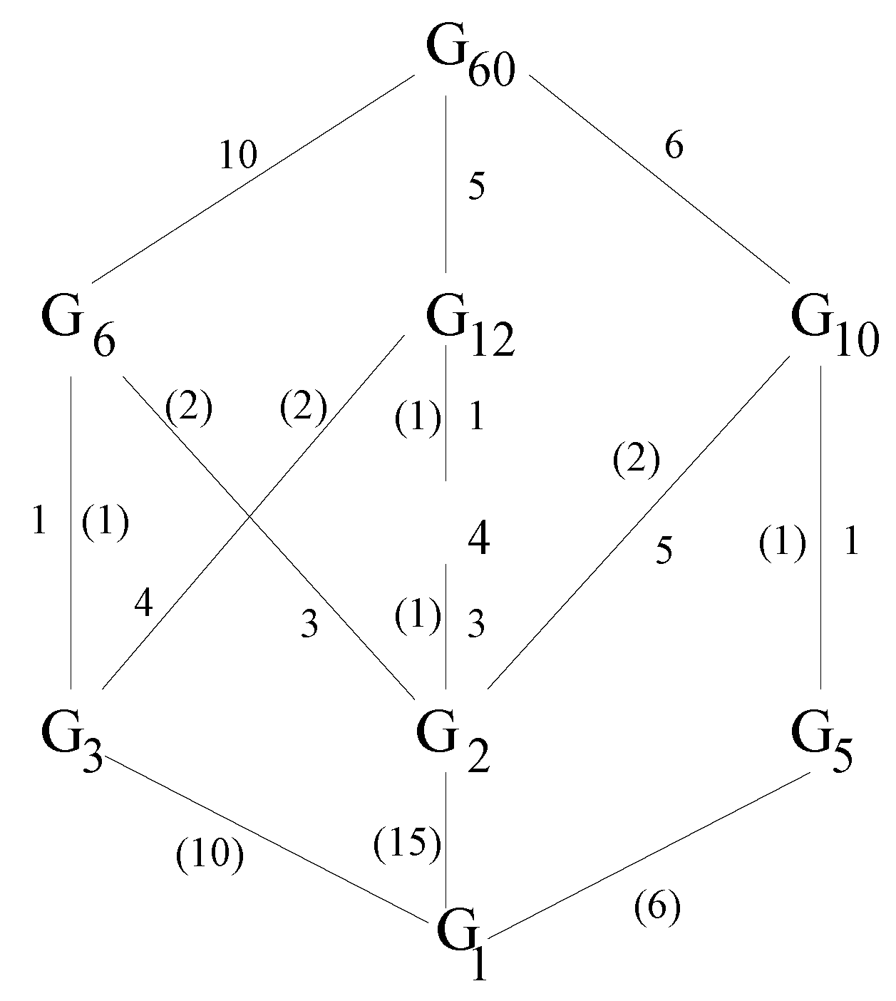
forms a lattice, ordered by inclusion. A partial Hasse diagram for this lattice
is shown in
Figure 10. The number on the edge joining
(below) and
(above) indicates the number of distinct subgroups of order
i contained in each subgroup of order
j. The number in parentheses on the edge joining
(below) and
(above) indicates the number of distinct subgroups of order
j containing each subgroup of order
i. The Möbius function of
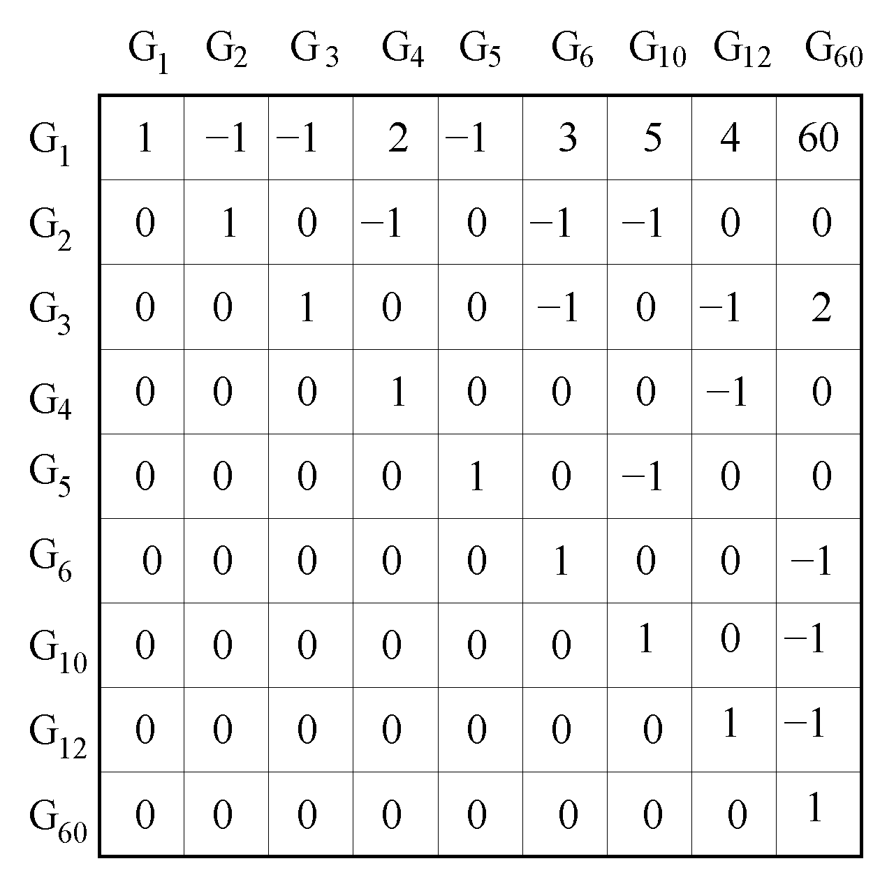
is shown in
Figure 11. The entry in the table corresponding to the row labeled
and column
is
.
Figure 10.
Partial Hasse diagram for the lattice of subgroups of the icosahedral group.
Figure 10.
Partial Hasse diagram for the lattice of subgroups of the icosahedral group.
Figure 11.
The values of the Möbius function of the subgroup lattice of .
Figure 11.
The values of the Möbius function of the subgroup lattice of .
Consider the case
,
i.e., for the
capsid. Using Theorem 7 and MAPLE software, the generating functions
were computed, and hence, their coefficients
, which count simplified assembly trees that are fixed by any copy of
, were also computed. Note that, since
, the number of orbits of
in its action on
X is
. Substituting these values into Theorem 6 and using the Möbius,
Figure 11 yields the numerical values for
, the number of simplified assembly trees over
X with
that are fixed by
, but by no other elements of
. In other words, these are the numbers of trees whose stabilizer in
is exactly
. Substituting these numbers
into Theorem 5, we arrive at the number of simplified assembly pathways of each possible size:


