Supersymmetric Quantum Mechanics and Solvable Models

Classification: PACS 03.65.-w, 47.10.-g, 11.30.Pb

1. Introduction

Supersymmetric quantum mechanics (SUSYQM) is a generalization of the factorization method commonly used for the harmonic oscillator. The factorization technique begun by Darboux [1] about one hundred years ago, and used by Schrödinger [2,3,4] in the 1940’s and Infeld and Hull in the 1950’s [5], could be considered a precursor of SUSYQM.

The current form of SUSYQM appeared in 1981 [6] as a model of dynamical symmetry breaking. It was developed further by the authors of [8,7] among others. This simplified model turned out to have important applications in quantum mechanics.

In the next section, we will describe the general formalism of SUSYQM and in Section 3 we introduce the shape invariance condition that makes a potential solvable. Section 4 is dedicated to a description of potential algebra and its connection to shape invariance. In Section 5 we will describe a method for determining solutions of the translational shape invariance condition. We will then conclude with the analysis of recently discovered shape invariant potentials that are inherently functions of .

2. Supersymmetric Quantum Mechanics

Throughout this paper, we use units such that . For the harmonic oscillator, the Hamiltonian [9] is factorized into and . Similarly, in the SUSYQM formalism [10,11] a general Hamiltonian is written as a product of and , where the function is known as the superpotential. The product is then given by

(1)

Thus, the product indeed reproduces the Hamiltonian above, provided the potential is related to the superpotential by . The product produces another Hamiltonian with . To see the underlying supersymmetry of this formalism, let us construct a generator and its adjont by:

(2)

Operators and generate the following supersymmetry algebra:

(3)

The groundstate energy of this Hamiltonian is then given by

(4)

Thus, the non-vanishing of the groundstate energy implies that either or , and hence signals the spontaneous breaking of the supersymmetry. We therefore require that to preserve unbroken supersymmetry.

The Hamiltonians and are intertwined; i.e., and . This leads to the following relationships among their eigenvalues and eigenfunctions [12]

(5)

Since H_± are products of the operator and its adjoint , their eigenvalues are either zero or positive [13]. The ground state eigenvalue of one of these Hamiltonians must be zero in order to have unbroken supersymmetry. Without loss of generality, we choose that Hamiltonian to be . Thus, we have

(6)

where is an arbitrary point in the domain and is the normalization constant that depends on the choice of . Thus, if is a normalizable groundstate, we have a system with unbroken supersymmetry. Its groundstate is zero and the operator annihilates the corresponding eigenstate . For all higher states of , as indicated in Equation (5), there is an one-to-one correspondence with the states of .

2.1. Example

Consider a system described by the superpotential , defined over the domain . Corresponding partner potentials are given by . This is a rather complicated potential, and rarely analyzed in quantum mechanics courses. However, for , the potential reduces to the infinite square well, with the bottom of the potential at and zero groundstate energy. We know that the corresponding eigenstates are given by and eigenvalues . Thus, using the familiarity with the relatively simpler potential , we are able to derive all of the eigenvalues and eigenfunctions of . Then the inter-relations expressed through Equation (5) enable us to determine eigenvalues and eigenfunctions of .

Although we assume that our Hamiltonians are hermitian, hermiticity is not necessary to generate real eigenvalues. Replacing the sufficient but not necessary condition of hermiticity with the weaker condition of PT symmetry, has led to the discovery of new potentials with real energy eigenvalues [14,15,16]. Considerable work has been done on the study of SI potentials with PT symmetry. In reference [17], the author examined the shape invariant hyperbolic Rosen-Morse potential as a case of exact solvability with PT invariance. In reference [18], the Scarf II potential was shown as an example of spontaneous PT-symmetry-breaking. The case of a square well with discrete PT symmetry but with intervals of non-hermiticity was shown in reference [19] to produce real eigenvalues. Authors of [20] constructed the spectrum of a square well of imaginary strength, to obtain the hierarchy of SI potentials, while authors of [21] constructed a set of solvable rational potentials, and related the PT symmetry condition to the condition that they be free of singularities. However, in this paper we limit ourselves to the case of hermitian Hamiltonians, i.e., real .

The remainder of this manuscript is devoted to the study of the shape invariance condition and its solutions.

3. Shape Invariance in Supersymmetric Quantum Mechanics

If the superpotential of a system obeys the condition

(7)

where , the system is called shape invariant [5,22,23,24]. Various forms of the function define classes of shape invariance. The most commonly discussed classes are:

From Equation (7) it follows that for a shape invariant system, the partner potentials and differ only by values of parameter and additive constants . In particular,

(8)

In terms of operators A_±, the shape invariance condition becomes

(9)

As we will see in Section 4, Equation (9) implies that for every shape invariant system, there is always an underlying potential algebra [28,30,29,32,31] that guarantees its solvability. In the rest of this section, we will show how shape invariance enables us to find the eigenvalues and eigenfunctions of the system.

3.1. Determination of Eigenvalues

From Equation (9), we see that Hamiltonians and differ only by the constant . We already know that . Let us determine the first excited state of ; i.e., . Hence, using [33], we find that the energy of the first excited state of and of the groundstate of both are given by . Similarly, to determine , we use the isospectrality condition (5) to relate it to . But by the shape invariance condition (9), = . Following the method used for determining , we find , and hence, . Extending this argument to higher excited states of , we get

(10)

3.2 Determination of Eigenfunctions

Again from Equation (9), we see that since and only differ by the constant , they must have common eigenfunctions. Hence, from Equation (6), we have . Then the isospectrality condition (5), requires . Iterating this procedure, we obtain

(11)

Thus, for a system with a given shape invariant superpotential, the eigenvalues and eigenfunctions can be determined analytically. This result makes it very important to find all such potentials. In the past, researchers had found a list of additive shape invariant potentials [10,11], mostly by trial and error [34,35]. In Section 5, we will discuss how to find solutions of Equation (9) for the additive case. Before that, however, in the next section we will show why the shape invariance condition leads to solvability.

4. Shape Invariance and Potential Algebra

We will now show that the symmetry behind the shape invariance is essential in building the algebraic structures known as potential algebras. As we will show below, a potential algebra is in general a deformation of a three-dimensional Lie algebra, whose representations yield the spectrum of the corresponding shape invariant system.

4.1. Building the Algebra

The starting point of our construct is the shape invariance condition given by Equation (9), which we rewrite as

(12)

where , and is a function that models the change of parameter . For example, if the change of parameter is a translation, .

The left hand side of Equation (12) resembles a commutation relation. This suggests that we use and to build the generators of the potential algebra. To transform the above shape invariance condition into an exact commutator, we replace operators and by

(13)

where is a constant parameter, is an auxiliary variable, and . The function will be appropriately chosen to emulate the relationship between parameters and . Thus, to generate , we multiplied the operator from right by and replaced the parameter by the differential operator . If we now compute the commutator between operators and , we find [36]

(14)

Observe now that the right hand side of Equation (14) matches the left hand side of Equation (12) provided that we make the following mappings

(15)

Since we know that , these mappings require that the function satisfy

(16)

Let us look at some examples to illustrate this procedure.

• Translation:

If the change of parameters is a translation, then the function that models it is the identity function

(17)

We have , which gives the desired change of parameters.

• Scaling:

For shape invariant potentials characterized by a scaling change of parameters, the corresponding function is the exponential

(18)

Indeed where we denoted .

• Cyclic:

Cyclic potentials form a series of shape invariant potentials that repeats after a cycle of iterations. These potentials appear also in connection with the dressing chain formalism [37]. To satisfy the cyclic parameter change, the function should obey . The projective map with specific constraints [38] on the parameters , and satisfies such a condition [27]. The function satisfying Equation (16) in this case is given by

(19)

where are solutions of the equation and is an arbitrary periodic function of with period .

• Other choices of parameters follow from more complicated choices for . For example taking

(20)

we obtain the change of parameters: .

Now, let us get back to the building of the potential algebra. In terms of operators and , the shape invariance condition (12) becomes:

(21)

Thus, the commutation relation of operators and generates an operator that has no -dependence. If we now define a third operator in terms of the operator , the shape invariance condition becomes simply one of the commutation relations of the potential algebra. In particular, if we define

(22)

where is an arbitrary constant, the three commutators among these generators are given by [39]

(23)

Putting together the above results, we arrive at the following

Lemma: To any shape invariant system characterized by

(24)

for which we can find a function such that for arbitrary parameters and , we can associate an algebra [40]generated by

(25)

(26)

(27)

satisfying the commutation relations

(28)

where

(29)

The function in Equation (29) is given by the shape invariance condition (24), while the function satisfies the compatibility equation: , where models the change of parameter of Equation (24).

As an example let us build the potential algebra corresponding to the Pöschl-Teller II potential. The potential

(30)

is generated by the superpotential , through , where . Its supersymmetric partner is given by

(31)

The shape invariance is now evident if we observe that . Therefore, in terms of and operators, the shape invariance (24) for the Pöschl-Teller II potential reads

(32)

Now we can identify the main objects of our model and build the corresponding algebra:

1. The parameters of the model are and , where is an arbitrary positive constant greater than so that is a positive quantity;

2. The change of parameter is thus given by . This is a translational change of parameter with the translation parameter . Translation implies that the function satisfying (16) is the identity function ;

3. From the concrete shape invariance condition (32) of this potential we get . Then, the function is given by if we choose the arbitrary constant ;

4. Defining and as prescribed by Equations (25) and (27), we obtain the differential realization of the algebra’s generators:

(33)

satisfying the commutation relations , and . Thus, shape invariance of this system implies that the system has a potential algebra given by [?, 41, 42].

4.2. Obtaining the Energy Spectrum from Algebra Representations

Once we know the potential algebra for a given potential, we can use its representations to obtain the energy spectrum for the Hamiltonian. Using Equations (25) and (26), we observe that

(34)

From the reciprocal of the mapping Equation (13), we obtain . Consequently, the spectrum of the operator gives the spectrum of the Hamiltonian. To find the concrete values for the energy, we need to know the action of individual operators and respectively on a set of eigenvectors of the operator . In this general case, , and commute with the Casimir operator given by

(35)

with the function (defined up to an additive constant) such that

(36)

It can be explicitly checked that does indeed commute with , and [41]. In a basis in which and are diagonal, play the role of raising and lowering operators, respectively. Operating on an arbitrary eigenstate we have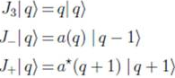

(37)

where we have used .

Keeping in mind that , and observing that , we see that in order to find the energies of the system one must find the coefficients . If we apply the third commutation relation of Equation (23) to , we obtain using Equation (36)

(38)

Next, we will determine the allowed values of and the corresponding values . Let us say corresponds to the lowest state in a given representation of the algebra. This implies that , which means . From Equation (38) we get

(39)

Iterating this procedure we can generate a general formula for

(40)

Substituting leads to

(41)

The profile of determines the dimension of the representation. For example, let us consider the two cases presented in Figure 1.

Figure 1. Generic behaviors of . Case (a) corresponds to a finite, and (b) to an infinite representation of the potential algebra.

Figure 1. Generic behaviors of . Case (a) corresponds to a finite, and (b) to an infinite representation of the potential algebra.

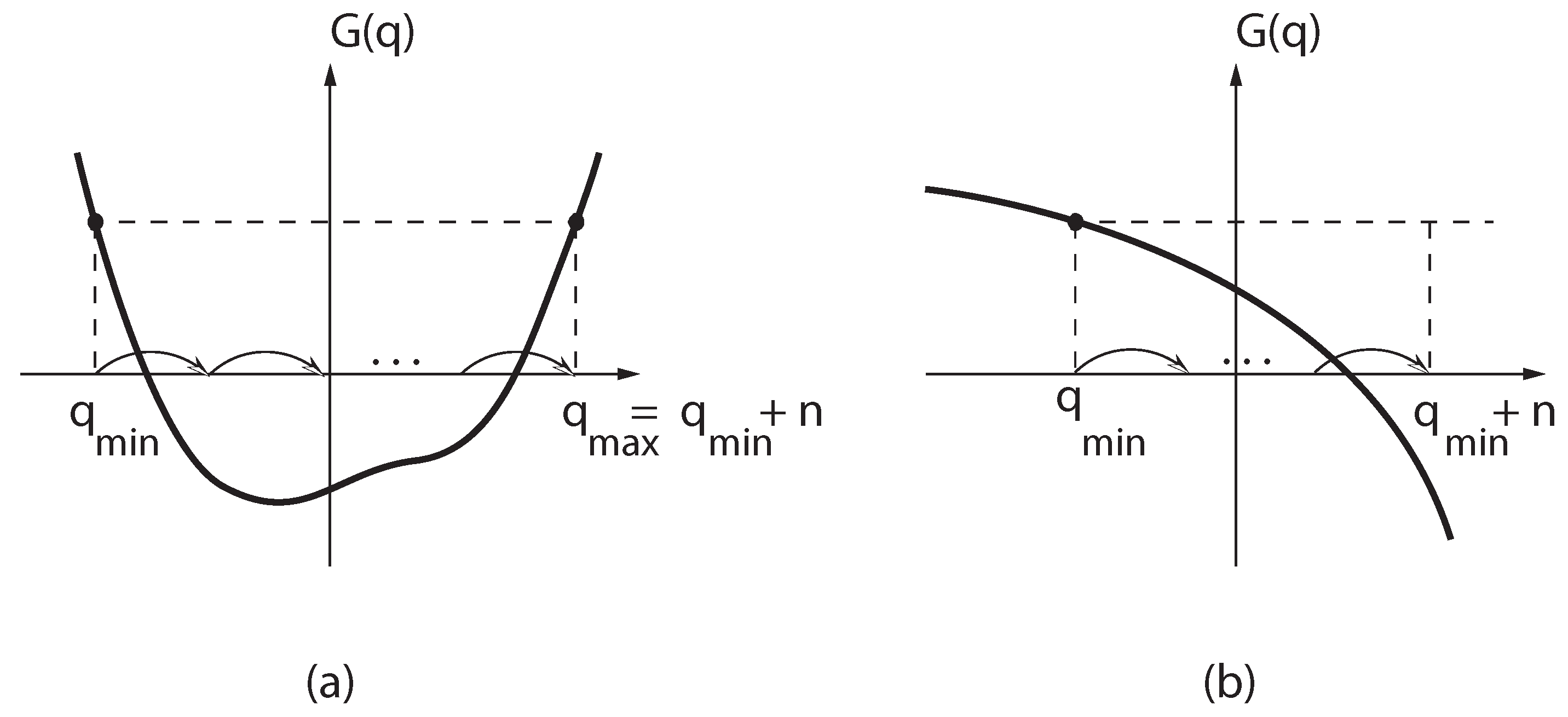One obtains the finite dimensional representations of Figure 1a, by starting from a point on the vs. graph corresponding to , and moving in integer steps parallel to the -axis to the point corresponding to . At the end points, , and we get a finite representation. If is decreasing monotonically, as in Figure 1b, there exists only one end point at . Starting from the value of can be increased in integer steps up to infinity. In this case we have an infinite dimensional representation. As in the finite case, labels the representation. The difference is that here takes continuous values. Similar arguments apply for a monotonically increasing function . Having the representation of the algebra associated with a characteristic model, we obtain, using Equation (41), the complete spectrum of the system.

For example, let us consider the scaling change of parameters . Consider the simple choice , where is a constant. This choice generates self-similar potentials studied in references [44,26,25]. In this case, combining Equation (18) with Equation (28) yields:

(42)

which is a deformation of the standard Lie algebra.

For this case, from Equations (42) and (36) one gets

(43)

Note that for scaling problems [25], one requires , which leads to . From the monotonically decreasing profile of the function , it follows that the unitary representations of this algebra are infinite dimensional. If we label the lowest weight state of the operator by , then . Without loss of generality we can choose the coefficients to be real. Then one obtains from (38) for an arbitrary

(44)

The spectrum of the Hamiltonian is given by

(45)

Therefore, the eigenenergies are

(46)

in agreement with the known results [25].

5. How Do We Find Additive Shape Invariant Superpotentials?

Since we have demonstrated the value of shape-invariant superpotentials, the question now becomes how to find such superpotentials. This question is equivalent to asking how to solve the difference-differential Equation (9) to find the list of desired superpotentials . For this section, we will restrict ourselves to considering cases of translational shape invariance. Before we embark on solving this equation, let us first note that quantum mechanical potentials generally have terms of two very different orders: One “large" and another “small". For example, the classical and quantum potentials for the radial oscillator system are and respectively. To make the transition from the quantum to the classical system, one takes the limit with the constraint that . Thus, the quantum Hamiltonian can be written as . This shows that in quantum mechanics, the potential generally has one small term that depends on [43]. In SUSYQM, since the potential is given by , the derivative term always brings in a factor of , even if the superpotential is independent of . In the following analysis, as we determine how to solve Equation (9) to find shape invariant superpotentials, we will consider the cases of -independent and -dependent superpotentials separately.

5.1. Known -Independent Shape Invariant Superpotentials

We begin our discussion of known shape invariant systems by considering only superpotentials that do not depend explicitly on , which we call “conventional” superpotentials. In Table 1 we list the known “conventional" superpotentials that meet this criterion.

Previous work [45,46,47] has proven that this list of conventional shape-invariant superpotentials is complete. We now show a new proof of this completeness which has the advantage of being significantly more straightforward and elegant than it predecessors.

Table 1. The complete family of -independent additive shape-invariant superpotentials.

Name	Superpotential
Harmonic Oscillator
Coulomb
-D oscillator
Morse
Rosen-Morse I
Rosen-Morse II
Eckart
Scarf I
Scarf II
Gen. Pöschl-Teller

Table 1. The complete family of -independent additive shape-invariant superpotentials.

Name	Superpotential
Harmonic Oscillator
Coulomb
-D oscillator
Morse
Rosen-Morse I
Rosen-Morse II
Eckart
Scarf I
Scarf II
Gen. Pöschl-Teller

5.2. New Proof of Completeness of the Conventional Shape-Invariant Superpotentials

Because of additive shape invariance, the dependence of on and is through the linear combination ; therefore, the derivatives of with respect to and are related by: . Since Equation (7) must hold for an arbitrary value of , if we assume that does not depend explicitly on , we can expand in powers of , and the coefficient of each power must separately vanish. Expanding the right hand side in powers of yields

(47)

(48)

(49)

Thus, all conventional additive shape invariant superpotentials are solutions of the above set of non-linear partial differential equations [46,47]. Although this represents an infinite set, note that if equations of and are satisfied, all others automatically follow. Therefore, we proceed to find all possible solutions to the two partial differential equations:

(50)

and

(51)

In doing so, we derive a new proof that the superpotentials shown in Table 1 are the only possible solutions.

The general solution to Equation (51) is

(52)

Therefore, to generate all shape invariant superpotentials, we need to determine all possible combinations of , , and that satisfiy Equation (50). We will ignore the case when both , and are constants, as this corresponds to a flat potential with no -dependence. We will also ignore the case in which , and are linearly dependent on each other; i.e., . In this case, . If we redefine , this case becomes equivalent to a superpotential with a shifted parameter and constant which will be considered shortly. We can therefore assume that and are linearly independent of each other without loss of generality. Note that from here onward, we will use lower case Greek letters to denote constants that are independent of both and .

To determine , we first focus on determining . To do so, we take two derivatives of (50) with respect to . This leads to the following differential equation:

where dots and primes represent derivatives taken with respect to and respectively. Since , this simplifies to:

(53)

Inserting the form of the general solution (52) into (53) yields

(54)

where is a function of , and is independent of . Since and are linearly independent, we find that there are only three possible ways for the left-hand-side of Equation (54) to be independent of :

• Case 1: is a constant and ;

• Case 2: is a constant and ;

• Case 3: Neither nor are not constants, but and .

For each of these cases we can determine the form of . Then we can determine and for these three cases. This we do by taking two derivatives of (50), this time one with respect to and another with respect to . This yields:

(55)

Inserting the form of the general solution (52) into (55) yields

(56)

Now, we will analyze each of the three cases in detail.

5.2.1. Case 1: X1 Is a Constant and

Let . Since cannot be a constant as well, Equation (54) requires . This leads to for some arbitrary constants , , , and . Inserting and into Equation (52) yields where .

We now find by inserting the above into Equation (50). This yields

or equivalently,

(57)

where .

Since is independent of , and the left side of (57) is a sum of four linearly independent functions of , and the term on the right-hand-side is independent of , the coefficient of each power of must separately be independent of . The linear term in therefore requires that be independent of . Since a constant leads to a trivial solution, we must have The remaining -dependent terms on the left side of (57), must be a constant:

(58)

The solution depends on the value of the constants and .

• Case 1A: In this case, , which is a trivial solution;

• Case 1B: In this case, so Defining yields the harmonic oscillator superpotential;

• Case 1C: The solution is then , . Therefore, For , this yields , where and . This is the Morse superpotential. Note that decreases as increases, and hence signals a finite number of eigenstates [48].

5.2.2. Case 2: Is Constant

In this case, let ; then Equation (54) requires . This yields . We now insert this form of and into (56) to get an ordinary differential equation in for :

or equivalently,

Integrating it once, we get

(59)

This equation can be simplified by setting . This leads to

(60)

The solutions for depend on the constant .

• Case 2A: In this case, The whole superpotential is then given by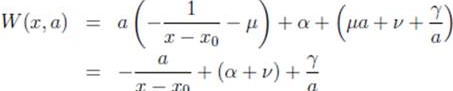

(61)

Setting and , and identifying , and , we get : the superpotential for Coulomb [49];

• Case 2B: In this case, we have either (Eckart) or (Rosen-Morse II). In the first case, the superpotential is given by , where we have set and . This is the well known Eckart potential. Similarly, the other solution with generates Rosen-Morse II;

• Case 2C: In this case, we obtain . An analysis similar to the previous case generates the superpotential for Rosen-Morse I.

5.2.3. Case 3: and Are not Constant, but and

In this case, since , and , we have . Therefore . In this case, Equation (56) yields

Integrating,

(62)

Thus, again we have

(63)

Note that this is the same differential equation as (60) and will therefore give the same solutions for as Case 2. However, in this case, (this is equivalent to choosing in Case 2) and is not constant. Instead, in each case we must plug our solutions for and into Equation (50), which yields

This equation is again simplified by setting , which yields

Since and are independent of , the terms linear in and the terms independent of on the left side of this equation must each separately be independent of . Therefore,

(64)

(65)

For different values of , we get different superpotentials:

• Case 3A: . We again get , where with an appropriate choice for the origin we have set . Equation (65) for becomes

(66)

Its solution is . With the identification , , , we get , the superpotential for the 3D-harmonic oscillator;

• Case 3B: As seen before, implies that or . By translation and scaling of , we can simplify the first solution to . Substituting in Equation (65), we get

(67)

where we have set The solution to the homogeneous equation is , and the particular solution is . Hence . Thus, the superpotential is given by , the General Pöschl-Teller potential given in Table 1. The second solution generates the Scarf II potential;

• Case 3C: A similar analysis for this case leads to Scarf I as the corresponding shape invariant superpotential.

Thus, we have generated all the superpotentials of Table 1 and shown that these are the only possible -independent solutions to the additive shape invariant condition.

5.3. -Dependent Superpotentials

In the previous section we generated the complete list of additive shape-invariant superpotentials that do not depend explicitly on . However, a new class of superpotentials was discovered by Quesne [50,51]. It has been shown [46] that these “extended" superpotentials obey the shape invariance condition in the form of Equation (7) only when is allowed to depend explicitly on . While this dependence is frequently ignored by the conventional notation that sets , we will show that this constraint results in important consequences for the energy spectrum of the resulting potentials. In each case, the new potential is isospectral with a potential that arises from one of the “conventional" superpotentials listed in Table 1. Authors of [52,53,54] have added an infinite number of potentials that belong in this class, and extended shape invariant potentials continue to be objects of intense research [55,56].

We now extend our formalism to include “extended" superpotentials that contain explicitly. To do so, we expand the superpotentials in powers of . Hence, we define

(68)

We will now substitute Equation (68) into the shape invariance condition given in Equation (7), for which we compute and . We obtain

and

Since , Expanding in powers of

Similarly,

We substitute these into Equation (7) and stipulate that the equation hold for any value of . After some significant algebraic manupulation we find that the following equation must be true separately for each positive integer value of :

(69)

For , we obtain

(70)

This equation is identical to Equation (50) for -independent ’s. We have already found a set of solutions for Equation (70) that includes all known -independent superpotentials. The extended cases [50,51] are solutions to (69) as well, as shown in [46]. Note that Equation (69) provides a consistency condition for all -dependent potentials; however, these are not easy to solve to determine new potentials.

Additionally, Equation (70) provides a constraint for the possible energy spectra of the extended potentials. from Equation (70), the function is given by

(71)

(72)

Thus, the function , and hence the energy of the system, is given entirely in terms of the -independent part of the superpotential. Hence, the eigenvalues are not affected by the -dependent extension of the superpotential.

Thus far, each of the known extended potentials contains a solution from Table 1 as the -independent term of the superpotential . Therefore, each of the expanded potentials is isospectral with its corresponding conventional potential. Future possibilities for finding new shape-invariant superpotentials fall into one of two categories:

1. Further extended superpotentials may be found based on the conventional superpotentials. In this case, the potentials derived from the extended superpotential will be isospectral with the potentials derived from the corresponding conventional superpotential;

2. While is required to satisfy Equation (70), which is equivalent to Equation (50) for -independent ’s, is not required to satisfy Equation (48). Rather, the additional constraints for an extended are supplied by Equation (69). It therefore may be possible to find an -dependent superpotential whose -independent term is not equivalent to a conventional superpotential. Intriguingly, it therefore may still be possible to discover shape-invariant systems with new energy spectra.

6. Summary and Conclusions

While supersymmetric quantum mechanics began as a simplified model to account for dynamical symmetry breaking, the application of this formalism to quantum mechanics has become an important field in its own right. In this manuscript we have reviewed research on supersymmetric quantum mechanics with a particular emphasis on the property of shape invariance. As we have shown, shape invariance is a sufficient condition for exact solvability of quantum mechanical problems; i.e., given a superpotential with shape invariance, all its eigenvalues and eigenfunctions can be determined analytically.

However, in its traditional form, the shape invariance condition Equation (7) is a difference-differential equation and is difficult to solve. It has recently been established that for additive shape-invariant superpotentials that do not explicitly depend on , this condition can be written as a set of local partial differential equations [45,46,47]. The solution to these equations showed that the list of such superpotentials was indeed complete. In this manuscript, we have presented a more straightforward proof of this result.

Since 2008, new sets of additive shape invariant potentials have been discovered [50,51,52,53,54]. We have reviewed the development of these “extended" shape-invariant systems and have provided an infinite set of partial differential equations that all extended potentials (where superpotentials are inherently functions of ) must obey [46,47]. We have also discussed the constraints placed on the energy spectra of these extended potentials as well as possibilities for finding additional as-yet-undiscovered cases of additive shape invariance.

It may also be possible to extend this method to other forms of shape invariance such as multiplicative or cyclic. For these, the potentials are generally not available in terms of known functions, except in very special cases ( for cyclic and limiting cases for multiplicative). It remains to be shown whether the shape invariance condition for these classes can be transformed from a difference-differential equation into a set of partial differential equations and be subjected to similar analysis.

References and Notes

- Darboux, G. Leçons sur la Théorie Général des Surfaces, 2nd ed; Gauthier-Villars: Paris, France, 1912. [Google Scholar]
- Schrödinger, E. A method of determining quantum-mechanical eigenvalues and eigenfunctions. Proc. R. Ir. Acad. 1940, A46, 9–16. [Google Scholar]
- Schrödinger, E. Further studies on solving eigenvalue problems by factorization. Proc. R. Ir. Acad. 1941, A46, 183–206. [Google Scholar]
- Schrödinger, E. The factorization of the hypergeometric equation. Proc. R. Ir. Acad. 1941, A47, 53–54. [Google Scholar]
- Infeld, L.; Hull, T.E. The factorization method. Rev. Mod. Phys. 1951, 23, 21–68. [Google Scholar]
- Witten, E. Dynamical breaking of supersymmetry. Nucl. Phys. 1981, B185, 513–554. [Google Scholar]
- Solomonson, P.; Van Holten, J.W. Fermionic coordinates and supersymmetry in quantum mechanics. Nucl. Phys. 1982, B196, 509–531. [Google Scholar]
- Cooper, F.; Freedman, B. Aspects of supersymmetric quantum mechanics. Ann. Phys. 1983, 146, 262–288. [Google Scholar]
- Note the constant
![]() has been added to the usual harmonic oscillator potential to insure that the groundstate energy of the system remains at zero. This constant allows us to factorize the Hamiltonian
has been added to the usual harmonic oscillator potential to insure that the groundstate energy of the system remains at zero. This constant allows us to factorize the Hamiltonian ![]() as a product of operators
as a product of operators ![]() and
and ![]() .
. - Cooper, F.; Khare, A.; Sukhatme, U. Supersymmetry in Quantum Mechanics; World Scientific: Singapore, 2001. [Google Scholar]
- Gangopadhyaya, A.; Mallow, J.; Rasinariu, C. Supersymmetric Quantum Mechanics: An Introduction; World Scientific: Singapore, 2010. [Google Scholar]
-
![]() Thus,
Thus, ![]() is an eigenstate of
is an eigenstate of ![]() with an eigenvalue
with an eigenvalue ![]() .
. -
![]() .
. - Bender, C.M.; Boettcher, S. Real spectra in non-hermitian hamiltonians having PT symmetry. Phys. Rev. Lett. 1998, 80, 5243–5246. [Google Scholar]
- Bender, C.M.; Brody, D.C.; Jones, H.F. Complex extension of quantum mechanics. Phys. Rev. Lett. 2002, 89, 270401–1. [Google Scholar]
- Bender, C.M.; Berry, M.V.; Mandilara, A. Generalized PT symmetry and real spectra. J. Phys. A 2002, 35, L467–L471. [Google Scholar]
- Znojil, M. SI potentials with PT symmetry. J. Phys. A 2000, 33, L61–L62. [Google Scholar]
- Levai, Z. Exact analytic study of the PT-symmetry-breaking mechanism. Czech. J. Phys. 2004, 54, 77–84. [Google Scholar]
- Znojil, M. Matching method and exact solvability of discrete Pt-symmetric square wells. J. Phys. A 2006, 39, 10247–10261. [Google Scholar]
- Quesne, C.; Bagchi, B.; Mallik, S.; Bila, H.; Jakubsky, V. PT supersymmetric partner of a short-range square well. Czech. J. Phys. 2005, 55, 1161–1166. [Google Scholar]
- Bagchi, B.; Quesne, C.; Roychoudhury, R. Isospectrality of conventional and new extended potentials, second-order supersymmetry and role of PT Symmetry. Pramana 2009, 73, 337–347. [Google Scholar]
- Miller, W., Jr. Lie Theory and Special Functions (Mathematics in Science and Engineering); Academic Press: New York,NY,USA, 1968. [Google Scholar]
- Gendenshtein, L.E. Derivation of exact spectra of the schrodinger equation by means of supersymmetry. JETP Lett. 1983, 38, 356–359. [Google Scholar]
- Gendenshtein, L.E.; Krive, I.V. Supersymmetry in quantum mechanics. Sov. Phys. Usp. 1985, 28, 645–666. [Google Scholar]
- Barclay, D.; Dutt, R.; Gangopadhyaya, A.; Khare, A.; Pagnamenta, A.; Sukhatme, U. New exactly solvable hamiltonians: Shape invariance and self-similarity. Phys. Rev. A 1993, 48, 2786–2797. [Google Scholar]
- Spiridonov, V.P. Exactly solvable potentials and quantum algebras. Phys. Rev. Lett. 1992, 69, 398–401. [Google Scholar]
- Sukhatme, U.P.; Rasinariu, C.; Khare, A. Cyclic shape invariant potentials. Phys. Lett. 1997, A234, 401–409. [Google Scholar]
- Gangopadhyaya, A.; Mallow, J.V.; Sukhatme, U.P. Supersymmetry and Integrable Models:. In Proceedings of Workshop on Supersymmetry and Integrable Models; Aratyn, H., Imbo, T.D., Keung, W.-Y., Sukhatme, U., Eds.; Springer-Verlag.
- Balantekin, A.B. Algebraic approach to shape invariance. Phys. Rev. A 1998, 57, 4188–4191. [Google Scholar]
- Gangopadhyaya, A.; Mallow, J.V.; Sukhatme, U.P. Translational shape invariance and the inherent potential algebra. Phys. Rev. A 1998, 58, 4287–4292. [Google Scholar]
- Chaturvedi, S.; Dutt, R.; Gangopadhyaya, A.; Panigrahi, P.; Rasinariu, C.; Sukhatme, U. Algebraic shape invariant models. Phys. Lett. 1998, A248, 109–113. [Google Scholar]
- Balantekin, A.; Candido Ribeiro, M.; Aleixo, A. Algebraic nature of shape-invariant and self-similar potentials. J. Phys. A 1999, 32, 2785–2790. [Google Scholar]
- We assume that as
![]() , the supersymmetry remains unbroken.
, the supersymmetry remains unbroken. - Dutt, R.; Khare, A.; Sukhatme, U. Supersymmetry, shape invariance and exactly solvable potentials. Am. J. Phys. 1998, 56, 163. [Google Scholar]
- Cooper, F.; Ginocchio, J.; Khare, A. Relationship between supersymmetry and solvable potentials. Phys. Rev. D 1987, 36, 2458. [Google Scholar]
- In the last line we have used the fact that
![]() . This implies that for any analytical function
. This implies that for any analytical function ![]() , we have
, we have ![]() .
. - Veselov, A.P.; Shabat, A.B. Dressing chains and spectral theory of the Schrödinger operator. Funct. Anal. Appl. 1993, 27, 81–96. [Google Scholar]
- These constraints are:
. - We have used
. - Dutt, R.; Gangopadhyaya, A.; Rasinariu, C.; Sukhatme, U. Coordinate realizations of deformed Lie algebras with three generators. Phys. Rev. A 1999, 60, 3482–3486. [Google Scholar] [CrossRef]
- Rocek, M. Representation theory of the nonlinear SU (2) algebra. Phys. Lett. B 1991, 255, 554–557. [Google Scholar]
- Adams, B.G.; Cizeka, J.; Paldus, J. Lie algebraic methods and their applications to simple quantum systems. Advances in Quantum Chemistry, 19th ed; Academic Press: New York,NY,USA, 1987. [Google Scholar]
- In some cases these are additive constants and subtracted away. If we provide a common floor to all potentials, demanding that their groundstate energies be zero, we will find that all known solvable potentials pick up a
![]() dependent term.
dependent term. - Shabat, A. The infinite-dimensional dressing dynamical system. Inverse Probl. 1992, 8, 303–308. [Google Scholar]
- Gangopadhyaya, A.; Mallow, J.V. Generating shape invariant potentials. Int. J. Mod. Phys. A 2008, 23, 4959–4978. [Google Scholar]
- Bougie, J.; Gangopadhyaya, A.; Mallow, J.V. Generation of a complete set of additive shape-invariant potentials from an euler equation. Phys. Rev. Lett. 2010, 210402–1. [Google Scholar]
- Bougie, J.; Gangopadhyaya, A.; Mallow, J.V. Method for generating additive shape invariant potentials from an euler equation. J. Phys. A 2012, 44, 275307–1. [Google Scholar]
- Normalizability of the groundstate
![]() requires that
requires that ![]() be greater than zero. Since an increase in
be greater than zero. Since an increase in ![]() decreases
decreases ![]() , there can only be a finite number of increases.
, there can only be a finite number of increases. - By substituting
![]() into Equation (50) we find that shape invariance requires that
into Equation (50) we find that shape invariance requires that ![]() .
. - Quesne, C. Exceptional orthogonal polynomials, exactly solvable potentials and supersymmetry. J. Phys. A 2008, 41, 392001–1. [Google Scholar]
- Quesne, C. Solvable rational potentials and exceptional orthogonal polynomials in supersymmetric quantum mechanics. Sigma 2009, 5, 084–1. [Google Scholar]
- Odake, S.; Sasaki, R. Infinitely many shape invariant discrete quantum mechanical systems and new exceptional orthogonal polynomials related to the wilson and Askey-Wilson polynomials. Phys. Lett. B 2009, 682, 130–136. [Google Scholar]
- Odake, S.; Sasaki, R. Another set of infinitely many exceptional (Xl) laguerre polynomials. Phys. Lett. B 2010, 684, 173–176. [Google Scholar]
- Tanaka, T. N-fold supersymmetry and quasi-solvability associated with X-2-laguerre polynomials. J. Math. Phys. 2010, 51, 032101–1. [Google Scholar]
- Sree Ranjani, S.; Panigrahi, P.; Khare, A.; Kapoor, A.; Gangopadhyaya, A. Exceptional orthogonal polynomials, QHJ formalism and SWKB quantization condition. J. Phys. A 2012, 055210–1. [Google Scholar]
- Shiv Chaitanya, K.; Sree Ranjani, S.; Panigrahi, P.; Radhakrishnan, R.; Srinivasan, V. Exceptional polynomials and SUSY quantum mechanics. Available online: http://arxiv.org/pdf/1110.3738.pdf (accessed on 2 August 2012).
© 2012 by the authors; licensee MDPI, Basel, Switzerland. This article is an open-access article distributed under the terms and conditions of the Creative Commons Attribution license (http://creativecommons.org/licenses/by/3.0/).
Share and Cite
Bougie, J.; Gangopadhyaya, A.; Mallow, J.; Rasinariu, C. Supersymmetric Quantum Mechanics and Solvable Models. Symmetry 2012, 4, 452-473. https://doi.org/10.3390/sym4030452
Bougie J, Gangopadhyaya A, Mallow J, Rasinariu C. Supersymmetric Quantum Mechanics and Solvable Models. Symmetry. 2012; 4(3):452-473. https://doi.org/10.3390/sym4030452
Chicago/Turabian StyleBougie, Jonathan, Asim Gangopadhyaya, Jeffry Mallow, and Constantin Rasinariu. 2012. "Supersymmetric Quantum Mechanics and Solvable Models" Symmetry 4, no. 3: 452-473. https://doi.org/10.3390/sym4030452
APA StyleBougie, J., Gangopadhyaya, A., Mallow, J., & Rasinariu, C. (2012). Supersymmetric Quantum Mechanics and Solvable Models. Symmetry, 4(3), 452-473. https://doi.org/10.3390/sym4030452