Defining the Symmetry of the Universal Semi-Regular Autonomous Asynchronous Systems

Abstract

The regular autonomous asynchronous systems are the non-deterministic Boolean dynamical systems and universality means the greatest in the sense of the inclusion. The paper gives four definitions of symmetry of these systems in a slightly more general framework, called semi-regularity, and also many examples.

1. Introduction

Switching theory has developed in the 1950s and the 1960s as a common effort of the mathematicians and the engineers of studying the switching circuits (a.k.a. asynchronous circuits) from digital electrical engineering. We are unaware of any existent mathematical work published after 1970 on what we call switching theory. The published works are written by engineers and their approach is always descriptive and unacceptable for the mathematicians. The label of switching theory has changed to asynchronous systems (or circuits) theory. One of the possible motivations of the situation consists in the fact that the important producers of digital equipments have stopped the dissemination of such researches.

Our interest in asynchronous systems had bibliography coming from the 1950s and the 1960s, as well as engineering works giving intuition, as well as mathematical works giving analogies. An interesting rendez-vous has happened when the asynchronous systems theory has met the dynamical systems theory, resulting in the so-called regular autonomous systems (a.k.a Boolean dynamical systems) where the vector field is $\Phi :{\{0,1\}}^n\to {\{0,1\}}^n$ and time is discrete or real, and we obtain the unbounded delay model of computation of $\Phi$ suggested by the engineers. The synchronous iterations of $\Phi :\Phi \circ \Phi ,\Phi \circ \Phi \circ \Phi ,\dots$ of the dynamical systems are replaced by asynchronous iterations in which each coordinate ${\Phi }_1,\dots ,{\Phi }_n$ is iterated independently on the others, in arbitrary finite time.

We denote with $\mathbf{B}=\{0,1\}$ the binary Boolean algebra, together with the discrete topology and with the usual algebraic laws:

$$\begin{array}{c}\begin{array}{cc}& \overline{}\\ 0& 1\\ 1& 0\end{array},\begin{array}{ccc}·& 0& 1\\ 0& 0& 0\\ 1& 0& 1\end{array},\begin{array}{ccc}\cup & 0& 1\\ 0& 0& 1\\ 1& 1& 1\end{array},\begin{array}{ccc}\oplus & 0& 1\\ 0& 0& 1\\ 1& 1& 0\end{array}\hfill \end{array}$$

(1)

We use the same notations for the laws that are induced from $\mathbf{B}$ on other sets, for example $\forall x\in {\mathbf{B}}^n$, $\forall y\in {\mathbf{B}}^n$,

$$\begin{array}{cc}\hfill \overline{x}& =(\overline{x_1},\dots ,\overline{x_n})\hfill \\ \hfill x\cup y& =(x_1\cup y_1,\dots ,x_n\cup y_n)\hfill \end{array}$$

etc. In Figure 1, we have drawn at (a) the logical gate NOT, i.e., the circuit that computes the logical complement and at (b) a circuit that makes use of logical gates NOT. The asynchronous system that models the circuit from (b) has the state portrait drawn at (c). In the state portraits, the arrows show the increase of (the discrete or continuous) time. The underlined coordinates $\underset{¯}{{\mu }_i}$ are these coordinates for which ${\Phi }_i({\mu }_i)\ne {\mu }_i$ and they are called excited, or enabled, or unstable. The coordinates ${\mu }_i$ that are not underlined fulfill by definition ${\Phi }_i({\mu }_i)={\mu }_i$ and they are called not excited, or not enabled, or stable. The existence of two underlined coordinates in $(0,0)$ shows that ${\Phi }_1(0,0)=1$ may be computed first, ${\Phi }_2(0,0)=1$ may be computed first, or ${\Phi }_1(0,0)$, ${\Phi }_2(0,0)$ may be computed simultaneously, thus when the system is in $(0,0)$, it may run in three different directions, which results in non-determinism.

Our present purpose is to define the symmetry of these systems.

2. Semi-Regular Systems

Notation 1

We denote ${\mathbf{N}}_{\_}=\{-1,0,1,2,\dots \}$.

Notation 2

${\chi }_A:\mathbf{R}\to \mathbf{B}$ is the notation of the characteristic function of the set $A\subset \mathbf{R}$: $\forall t\in \mathbf{R},{\chi }_A(t)=\left\{\begin{array}{c}0,ift\notin A\\ 1,ift\in A\end{array}\right..$

Notation 3

We denote with ${\overline{\Pi }}_n$ the set of the sequences $\alpha ={\alpha }^0,{\alpha }^1,\dots ,$ ${\alpha }^k,$ $\dots \in {\mathbf{B}}^n.$

Notation 4

The set of the real sequences $t_0<t_1<\dots <t_k<\dots$ that are unbounded from above is denoted with $Seq$.

Notation 5

We use the notation ${\overline{P}}_n$ for the set of the functions $\rho :\mathbf{R}\to {\mathbf{B}}^n$ having the property that $\alpha \in {\overline{\Pi }}_n$ and $(t_k)\in Seq$ exist with $\forall t\in \mathbf{R},$

$$\rho (t)={\alpha }^0{\chi }_{\left\{t_0\right\}}(t)\oplus {\alpha }^1{\chi }_{\left\{t_1\right\}}(t)\oplus \dots \oplus {\alpha }^k{\chi }_{\left\{t_k\right\}}(t)\oplus \dots$$

(2)

Definition 6

Let $\Phi :{\mathbf{B}}^n\to {\mathbf{B}}^n$ be a function. For $\nu \in {\mathbf{B}}^n,\nu =({\nu }_1,\dots ,{\nu }_n)$ we define the function ${\Phi }^{\nu }:{\mathbf{B}}^n\to {\mathbf{B}}^n$ by $\forall \mu \in {\mathbf{B}}^n,$

$${\Phi }^{\nu }(\mu )=(\overline{{\nu }_1}{\mu }_1\oplus {\nu }_1{\Phi }_1(\mu ),\dots ,\overline{{\nu }_n}{\mu }_n\oplus {\nu }_n{\Phi }_n(\mu ))$$

Remark 7

For any $\mu \in {\mathbf{B}}^n,\nu \in {\mathbf{B}}^n$ and $i\in \{1,\dots ,n\},$ if ${\nu }_i=0,$ then ${\Phi }_i^{\nu }(\mu )={\mu }_i$ i.e., ${\Phi }_i(\mu )$ is not computed and if ${\nu }_i=1,$ then ${\Phi }_i^{\nu }(\mu )={\Phi }_i(\mu )$ i.e., ${\Phi }_i(\mu )$ is computed. This is the meaning of asynchronicity.

Definition 8

Let $\alpha \in {\overline{\Pi }}_n.$ The function ${\widehat{\Phi }}^{\alpha }:{\mathbf{B}}^n\times {\mathbf{N}}_{\_}\to {\mathbf{B}}^n$ defined by $\forall \mu \in {\mathbf{B}}^n,\forall k\in {\mathbf{N}}_{\_},$

$$\left\{\begin{array}{c}{\widehat{\Phi }}^{\alpha }(\mu ,-1)=\mu ,\hfill \\ {\widehat{\Phi }}^{\alpha }(\mu ,k+1)={\Phi }^{{\alpha }^{k+1}}({\widehat{\Phi }}^{\alpha }(\mu ,k))\hfill \end{array}\right.$$

(3)

is called discrete time $\alpha -$semi-orbit of $\mu .$ We consider also the sequence $(t_k)\in Seq$ and the function $\rho \in {\overline{P}}_n$ from Equation (2), for which the function ${\Phi }^{\rho }:{\mathbf{B}}^n\times \mathbf{R}\to {\mathbf{B}}^n$ is defined by: $\forall \mu \in {\mathbf{B}}^n,\forall t\in \mathbf{R},$

$$\begin{array}{cc}\hfill {\Phi }^{\rho }(\mu ,t)=& {\widehat{\Phi }}^{\alpha }(\mu ,-1){\chi }_{(-\infty ,t_0)}(t)\oplus {\widehat{\Phi }}^{\alpha }(\mu ,0){\chi }_{[t_0,t_1)}(t)\oplus \hfill \\ & \oplus {\widehat{\Phi }}^{\alpha }(\mu ,1){\chi }_{[t_1,t_2)}(t)\oplus \dots \oplus {\widehat{\Phi }}^{\alpha }(\mu ,k){\chi }_{[t_k,t_{k+1})}(t)\oplus \dots \hfill \end{array}$$

(4)

${\Phi }^{\rho }$ is called continuous time $\rho -$semi-orbit of $\mu .$

Definition 9

The discrete time and the continuous time universal semi-regular autonomous asynchronous systems associated to Φ are defined by

$$\begin{array}{cc}\hfill {\widehat{\overline{\Xi }}}_{\Phi }& =\left\{{\widehat{\Phi }}^{\alpha }(\mu ,·)\right|\mu \in {\mathbf{B}}^n,\alpha \in {\overline{\Pi }}_n\}\hfill \\ \hfill {\overline{\Xi }}_{\Phi }& =\left\{{\Phi }^{\rho }(\mu ,·)\right|\mu \in {\mathbf{B}}^n,\rho \in {\overline{P}}_n\}\hfill \end{array}$$

Remark 10

${\widehat{\overline{\Xi }}}_{\Phi },$ ${\overline{\Xi }}_{\Phi }$ and Φ are usually identified.

Example 11

In Figure 2 we have drawn at (a) the AND gate that computes the logical intersection, at (b) a circuit with two gates and at (c) the state portrait of $\Phi :{\mathbf{B}}^2\to {\mathbf{B}}^2,\forall ({\mu }_1,{\mu }_2)\in {\mathbf{B}}^2,\Phi ({\mu }_1,{\mu }_2)=(0,1).$ We conclude that

$$\begin{array}{cc}\hfill {\overline{\Xi }}_{\Phi }=& \{({\mu }_1,{\mu }_2){\chi }_{(-\infty ,t_0)}\oplus ({\mu }_1{\lambda }_1,{\mu }_2\cup {\lambda }_2){\chi }_{[t_0,t_1)}\oplus \hfill \\ & \oplus ({\mu }_1{\lambda }_1{\nu }_1,{\mu }_2\cup {\lambda }_2\cup {\nu }_2){\chi }_{[t_1,\infty )}|\mu ,\lambda ,\nu \in {\mathbf{B}}^2,t_0,t_1\in \mathbf{R},t_0<t_1\}\hfill \end{array}$$

since the first coordinate might finally decrease its value and the second coordinate might finally increase its value, but the order and the time instant when these things happen are arbitrary.

3. Anti-Semi-Regular Systems

Definition 12

Let $\Phi :{\mathbf{B}}^n\to {\mathbf{B}}^n,\alpha \in {\overline{\Pi }}_n,(t_k)\in Seq$ and $\rho \in {\overline{P}}_n$ from Equation (2). The function ${}^{*}{\widehat{\Phi }}^{\alpha }:{\mathbf{B}}^n\times {\mathbf{N}}_{\_}\to {\mathbf{B}}^n$ that satisfies $\forall \mu \in {\mathbf{B}}^n,\forall k\in {\mathbf{N}}_{\_},$

$$\left\{\begin{array}{c}{}^{*}{\widehat{\Phi }}^{\alpha }(\mu ,-1)=\mu \hfill \\ {\Phi }^{{\alpha }^{k+1}}{(}^{*}{\widehat{\Phi }}^{\alpha }(\mu ,k+1))={}^{*}{\widehat{\Phi }}^{\alpha }(\mu ,k)\hfill \end{array}\right.$$

(5)

is called discrete time $\alpha -$anti-semi-orbit of μ and the function ${}^{*}{\Phi }^{\rho }:{\mathbf{B}}^n\times \mathbf{R}\to {\mathbf{B}}^n$ that satisfies $\forall \mu \in {\mathbf{B}}^n,\forall t\in \mathbf{R},$

$$\begin{array}{cc}\hfill {}^{*}{\Phi }^{\rho }(\mu ,t)=& {}^{*}{\widehat{\Phi }}^{\alpha }(\mu ,-1){\chi }_{(-\infty ,t_0)}(t)\oplus {}^{*}{\widehat{\Phi }}^{\alpha }(\mu ,0){\chi }_{[t_0,t_1)}(t)\oplus \hfill \\ & \oplus {}^{*}{\widehat{\Phi }}^{\alpha }(\mu ,1){\chi }_{[t_1,t_2)}(t)\oplus \dots \oplus {}^{*}{\widehat{\Phi }}^{\alpha }(\mu ,k){\chi }_{[t_k,t_{k+1})}(t)\oplus \dots \hfill \end{array}$$

(6)

is called continuous time $\rho -$anti-semi-orbit of $\mu .$

Remark 13

We compare the semi-orbits and the anti-semi-orbits now and see that they run both from the past to the future, but the cause-effect relation is different: in ${\widehat{\Phi }}^{\alpha },{\Phi }^{\rho }$ the cause is in the past and the effect is in the future, while in ${}^{*}{\widehat{\Phi }}^{\alpha },$ ${}^{*}{\Phi }^{\rho }$ the cause is in the future and the effect is in the past.

Definition 14

The discrete time and the continuous time universal anti-semi-regular autonomous asynchronous systems associated to Φ are defined by

$$\begin{array}{cc}\hfill {}^{*}{\widehat{\overline{\Xi }}}_{\Phi }& ={\{}^{*}{\widehat{\Phi }}^{\alpha }(\mu ,·)|\mu \in {\mathbf{B}}^n,\alpha \in {\overline{\Pi }}_n\}\hfill \\ \hfill {}^{*}{\overline{\Xi }}_{\Phi }& ={\{}^{*}{\Phi }^{\rho }(\mu ,·)|\mu \in {\mathbf{B}}^n,\rho \in {\overline{P}}_n\}\hfill \end{array}$$

Example 15

In Figure 3 we have drawn at (a) the circuit and at (b) the state portrait of $\mathrm{\Psi }:{\mathbf{B}}^2\to {\mathbf{B}}^2$, $\forall ({\mu }_1,{\mu }_2)\in {\mathbf{B}}^2,$ $\mathrm{\Psi }({\mu }_1,{\mu }_2)=(1,0)$ for which

$$\begin{array}{cc}\hfill {\overline{\Xi }}_{\mathrm{\Psi }}=& \{({\mu }_1,{\mu }_2){\chi }_{(-\infty ,t_0)}\oplus ({\mu }_1\cup {\lambda }_1,{\mu }_2{\lambda }_2){\chi }_{[t_0,t_1)}\oplus \hfill \\ & \oplus ({\mu }_1\cup {\lambda }_1\cup {\nu }_1,{\mu }_2{\lambda }_2{\nu }_2){\chi }_{[t_1,\infty )}|\mu ,\lambda ,\nu \in {\mathbf{B}}^2,t_0,t_1\in \mathbf{R},t_0<t_1\}\hfill \end{array}$$

The arrows in Figure 2(c) and Figure 3(b) are the same, but with a different sense and we note that ${\overline{\Xi }}_{\mathrm{\Psi }}=$ ${}^{*}{\overline{\Xi }}_{\Phi },$ where Φ is the one from Example 11.

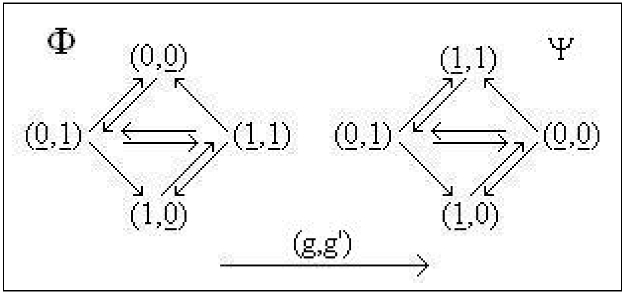
4. Isomorphisms and Anti-Isomorphisms

Definition 16

Let $g:{\mathbf{B}}^n\to {\mathbf{B}}^n.$ It defines the functions $\widehat{g}:{\overline{\Pi }}_n\to {\overline{\Pi }}_n,\forall \alpha \in {\overline{\Pi }}_n,\forall k\in \mathbf{N},$

$$\widehat{g}(\alpha )(k)=g({\alpha }^k)$$

$\tilde{g}:{\overline{P}}_n\to {\overline{P}}_n,\forall \rho \in {\overline{P}}_n,\forall t\in \mathbf{R},$

$$\tilde{g}(\rho )(t)=\left\{\begin{array}{cc}(0,\dots ,0),\hfill & \mathit{if}\rho (t)=(0,\dots ,0)\hfill \\ g(\rho (t)),\hfill & \mathit{otherwise}\hfill \end{array}\right.$$

and $g:{({\mathbf{B}}^n)}^{\mathbf{R}}\to {({\mathbf{B}}^n)}^{\mathbf{R}},\forall x\in {({\mathbf{B}}^n)}^{\mathbf{R}},\forall t\in \mathbf{R},$

$$g(x)(t)=g(x(t))$$

Theorem 17

Let $\Phi ,\mathrm{\Psi },g,g^{\prime }:{\mathbf{B}}^n\to {\mathbf{B}}^n.$ The following statements are equivalent:

(a) 

$\forall \nu \in {\mathbf{B}}^n,$ the diagram

$$\begin{array}{ccc}{\mathbf{B}}^n& \stackrel{{\Phi }^{\nu }}{\to }& {\mathbf{B}}^n\\ g\downarrow & & \downarrow g\\ {\mathbf{B}}^n& \stackrel{{\mathrm{\Psi }}^{g^{\prime }(\nu )}}{\to }& {\mathbf{B}}^n\end{array}$$

is commutative;

(b) 

$\forall \mu \in {\mathbf{B}}^n,\forall \alpha \in {\overline{\Pi }}_n,\forall k\in {\mathbf{N}}_{\_},$

$$g({\widehat{\Phi }}^{\alpha }(\mu ,k))={\widehat{\mathrm{\Psi }}}^{\widehat{g^{\prime }}(\alpha )}(g(\mu ),k)$$

(c) 

$\forall \mu \in {\mathbf{B}}^n,$

$$g(\mu )={\mathrm{\Psi }}^{g^{\prime }(0,\dots ,0)}(g(\mu ))$$

and $\forall \mu \in {\mathbf{B}}^n,\forall \rho \in {\overline{P}}_n,\forall t\in \mathbf{R},$

$$g({\Phi }^{\rho }(\mu ,t))={\mathrm{\Psi }}^{\widetilde{g^{\prime }}(\rho )}(g(\mu ),t)$$

Proof. 

(a)⟹(b): We fix arbitrarily $\mu \in {\mathbf{B}}^n,$ $\alpha \in {\overline{\Pi }}_n$ and we use the induction on $k\ge -1$. For $k=-1$, (b) becomes $g(\mu )=g(\mu )$, thus we suppose that it is true for k and we prove it for $k+1$:

$$\begin{array}{cc}\hfill g({\widehat{\Phi }}^{\alpha }(\mu ,k+1))& =g({\Phi }^{{\alpha }^{k+1}}({\widehat{\Phi }}^{\alpha }(\mu ,k)))={\mathrm{\Psi }}^{g^{\prime }({\alpha }^{k+1})}(g({\widehat{\Phi }}^{\alpha }(\mu ,k)))\hfill \\ & ={\mathrm{\Psi }}^{g^{\prime }({\alpha }^{k+1})}({\widehat{\mathrm{\Psi }}}^{\widehat{g^{\prime }}(\alpha )}(g(\mu ),k))={\widehat{\mathrm{\Psi }}}^{\widehat{g^{\prime }}(\alpha )}(g(\mu ),k+1)\hfill \end{array}$$

(b)⟹(c): The first statement results from (b) if we take ${\alpha }^0=(0,\dots ,0)$ and $k=0.$ In order to prove the second statement, let $\mu \in {\mathbf{B}}^n$ and $\rho \in {\overline{P}}_n$ be arbitrary, thus Equation (2) holds with $(t_k)\in Seq,\rho (t_0),\dots ,\rho (t_k),\dots \in {\overline{\Pi }}_n.$ If $\forall t\in \mathbf{R},\rho (t)=(0,\dots ,0)$ the statement to prove takes the form $g(\mu )=g(\mu )$ so that we can suppose now that a finite or an infinite number of $\rho (t_k)$ are $\ne (0,\dots ,0).$ In the case $\forall k\in \mathbf{N},\rho (t_k)\ne (0,\dots ,0)$ that does not restrict the generality of the proof, we have that

$$\widetilde{g^{\prime }}(\rho )(t)=g^{\prime }(\rho (t_0)){\chi }_{\left\{t_0\right\}}(t)\oplus \dots \oplus g^{\prime }(\rho (t_k)){\chi }_{\left\{t_k\right\}}(t)\oplus \dots$$

(7)

is an element of ${\overline{P}}_n$ and

$$\begin{array}{cc}\hfill g({\Phi }^{\rho }(\mu ,t))& =g(\mu {\chi }_{(-\infty ,t_0)}(t)\oplus {\widehat{\Phi }}^{\alpha }(\mu ,0){\chi }_{[t_0,t_1)}(t)\oplus \dots \oplus {\widehat{\Phi }}^{\alpha }(\mu ,k){\chi }_{[t_k,t_{k+1})}(t)\oplus \dots )\hfill \\ & =g(\mu ){\chi }_{(-\infty ,t_0)}(t)\oplus g({\widehat{\Phi }}^{\alpha }(\mu ,0)){\chi }_{[t_0,t_1)}(t)\oplus \dots \oplus g({\widehat{\Phi }}^{\alpha }(\mu ,k)){\chi }_{[t_k,t_{k+1})}(t)\oplus \dots \hfill \\ & =g(\mu ){\chi }_{(-\infty ,t_0)}(t)\oplus {\widehat{\mathrm{\Psi }}}^{\widehat{g^{\prime }}(\alpha )}(g(\mu ),0){\chi }_{[t_0,t_1)}(t)\oplus \dots \oplus {\widehat{\mathrm{\Psi }}}^{\widehat{g^{\prime }}(\alpha )}(g(\mu ),k){\chi }_{[t_k,t_{k+1})}(t)\oplus \dots \hfill \\ & ={\mathrm{\Psi }}^{\widetilde{g^{\prime }}(\rho )}(g(\mu ),t)\hfill \end{array}$$

(c)⟹(a): Let $\nu ,\mu \in {\mathbf{B}}^n$ be arbitrary and fixed and we consider $\rho \in {\overline{P}}_n$ given by Equation (2), with $(t_k)\in Seq$ fixed, $\rho (t_0)=\nu$ and $\forall k\ge 1,\rho (t_k)\ne (0,\dots ,0)$. We have

$$\begin{array}{cc}\hfill g({\Phi }^{\rho }(\mu ,t))& =g(\mu {\chi }_{(-\infty ,t_0)}(t)\oplus {\Phi }^{\nu }(\mu ){\chi }_{[t_0,t_1)}(t)\oplus {\widehat{\Phi }}^{\alpha }(\mu ,1){\chi }_{[t_1,t_2)}(t)\oplus \dots )\hfill \\ & =g(\mu ){\chi }_{(-\infty ,t_0)}(t)\oplus g({\Phi }^{\nu }(\mu )){\chi }_{[t_0,t_1)}(t)\oplus g({\widehat{\Phi }}^{\alpha }(\mu ,1)){\chi }_{[t_1,t_2)}(t)\oplus \dots \hfill \end{array}$$

(8)

Case (i) $\nu =(0,\dots ,0)$, the commutativity of the diagram is equivalent with the first statement of (c).

Case(ii) $\nu \ne (0,\dots ,0)$,

$$\begin{array}{cc}\hfill \widetilde{g^{\prime }}(\rho )(t)& =g^{\prime }(\rho (t))\hfill \\ & =g^{\prime }(\nu ){\chi }_{\left\{t_0\right\}}(t)\oplus g^{\prime }(\rho (t_1)){\chi }_{\left\{t_1\right\}}(t)\oplus \dots \hfill \\ \hfill {\mathrm{\Psi }}^{\widetilde{g^{\prime }}(\rho )}(g(\mu ),t)& =g(\mu ){\chi }_{(-\infty ,t_0)}(t)\oplus {\mathrm{\Psi }}^{g^{\prime }(\nu )}(g(\mu )){\chi }_{[t_0,t_1)}(t)\oplus {\widehat{\mathrm{\Psi }}}^{\widehat{g^{\prime }}(\alpha )}(g(\mu ),1){\chi }_{[t_1,t_2)}(t)\oplus \dots \hfill \end{array}$$

and from Equation (8), for $t\in [t_0,t_1),$ we obtain

$$g({\Phi }^{\nu }(\mu ))={\mathrm{\Psi }}^{g^{\prime }(\nu )}(g(\mu ))$$

Definition 18

We consider the functions $\Phi ,\mathrm{\Psi }:{\mathbf{B}}^n\to {\mathbf{B}}^n.$ If $g,g^{\prime }:{\mathbf{B}}^n\to {\mathbf{B}}^n$ bijective exist such that one of the equivalent properties (a), (b) or (c) from Theorem 17 is satisfied, then we say that the couple $(g,g^{\prime })$ defines an isomorphism from ${\widehat{\overline{\Xi }}}_{\Phi }$ to ${\widehat{\overline{\Xi }}}_{\mathrm{\Psi }},$ or from ${\overline{\Xi }}_{\Phi }$ to ${\overline{\Xi }}_{\mathrm{\Psi }},$ or from Φ to $\mathrm{\Psi }.$ We use the notation $\overline{Iso}(\Phi ,\mathrm{\Psi })$ for the set of these couples and we also denote with $\overline{Aut}(\Phi )=\overline{Iso}(\Phi ,\Phi )$ the set of the automorphisms of ${\widehat{\overline{\Xi }}}_{\Phi },$ ${\overline{\Xi }}_{\Phi },$ or $\Phi .$

Theorem 19

For $\Phi ,\mathrm{\Psi },g,g^{\prime }:{\mathbf{B}}^n\to {\mathbf{B}}^n$, the following statements are equivalent:

(a) $\forall \nu \in {\mathbf{B}}^n,$ the diagram is commutative;

$$\begin{array}{ccc}{\mathbf{B}}^n& \stackrel{{\Phi }^{\nu }}{\to }& {\mathbf{B}}^n\\ g\downarrow & & \downarrow g\\ {\mathbf{B}}^n& \stackrel{{\mathrm{\Psi }}^{g^{\prime }(\nu )}}{⟵}& {\mathbf{B}}^n\end{array}$$

(b) $\forall \mu \in {\mathbf{B}}^n,\forall \alpha \in {\overline{\Pi }}_n,\forall k\in {\mathbf{N}}_{\_},$

$$g(\mu )={}^{*}{\widehat{\mathrm{\Psi }}}^{\widehat{g^{\prime }}(\alpha )}(g({\widehat{\Phi }}^{\alpha }(\mu ,k)),k)$$

(c) $\forall \mu \in {\mathbf{B}}^n,$

$$g(\mu )={\mathrm{\Psi }}^{g^{\prime }(0,\dots ,0)}(g(\mu ))$$

and $\forall \mu \in {\mathbf{B}}^n,\forall \rho \in {\overline{P}}_n,\forall t\in \mathbf{R},$

$$g(\mu )={}^{*}{\mathrm{\Psi }}^{\widetilde{g^{\prime }}(\rho )}(g({\Phi }^{\rho }(\mu ,t)),t)$$

Proof. 

(a)⟹(b): We fix arbitrarily $\mu \in {\mathbf{B}}^n,$ $\alpha \in {\overline{\Pi }}_n$ and we use the induction on $k\ge -1.$ In the case $k=-1$ the equality to be proved is satisfied

$$g(\mu )=g({\widehat{\Phi }}^{\alpha }(\mu ,-1))={\widehat{\mathrm{\Psi }}}^{\widehat{g^{\prime }}(\alpha )}(g({\widehat{\Phi }}^{\alpha }(\mu ,-1)),-1)$$

thus we presume that the statement is true for k and we prove it for $k+1.$ We have:

$$\begin{array}{cc}\hfill g(\mu )& ={}^{*}{\widehat{\mathrm{\Psi }}}^{\widehat{g^{\prime }}(\alpha )}(g({\widehat{\Phi }}^{\alpha }(\mu ,k)),k)\hfill \\ & ={}^{*}{\widehat{\mathrm{\Psi }}}^{\widehat{g^{\prime }}(\alpha )}({\mathrm{\Psi }}^{g^{\prime }({\alpha }^{k+1})}(g({\Phi }^{{\alpha }^{k+1}}({\widehat{\Phi }}^{\alpha }(\mu ,k)))),k)\hfill \\ & ={}^{*}{\widehat{\mathrm{\Psi }}}^{\widehat{g^{\prime }}(\alpha )}(g({\widehat{\Phi }}^{\alpha }(\mu ,k+1)),k+1)\hfill \end{array}$$

The proof is similar with the proof of Theorem 17.

Definition 20

Let $\Phi ,\mathrm{\Psi }:{\mathbf{B}}^n\to {\mathbf{B}}^n.$ If $g,g^{\prime }:{\mathbf{B}}^n\to {\mathbf{B}}^n$ bijective exist such that one of the equivalent properties (a), (b) or (c) from Theorem 19 is fulfilled, we say that the couple $(g,g^{\prime })$ defines an anti-isomorphism from ${\widehat{\overline{\Xi }}}_{\Phi }$ to ${}^{*}{\widehat{\overline{\Xi }}}_{\mathrm{\Psi }},$ or from ${\overline{\Xi }}_{\Phi }$ to ${}^{*}{\overline{\Xi }}_{\mathrm{\Psi }},$ or from Φ to $\mathrm{\Psi }.$ We use the notation ${}^{*}\overline{Iso}(\Phi ,\mathrm{\Psi })$ for these couples and we also denote with ${}^{*}\overline{Aut}(\Phi )=$ ${}^{*}\overline{Iso}(\Phi ,\Phi )$ the set of the anti-automorphisms of ${\widehat{\overline{\Xi }}}_{\Phi },$ ${\overline{\Xi }}_{\Phi }$ or Φ.

5. Symmetry and Anti-Symmetry

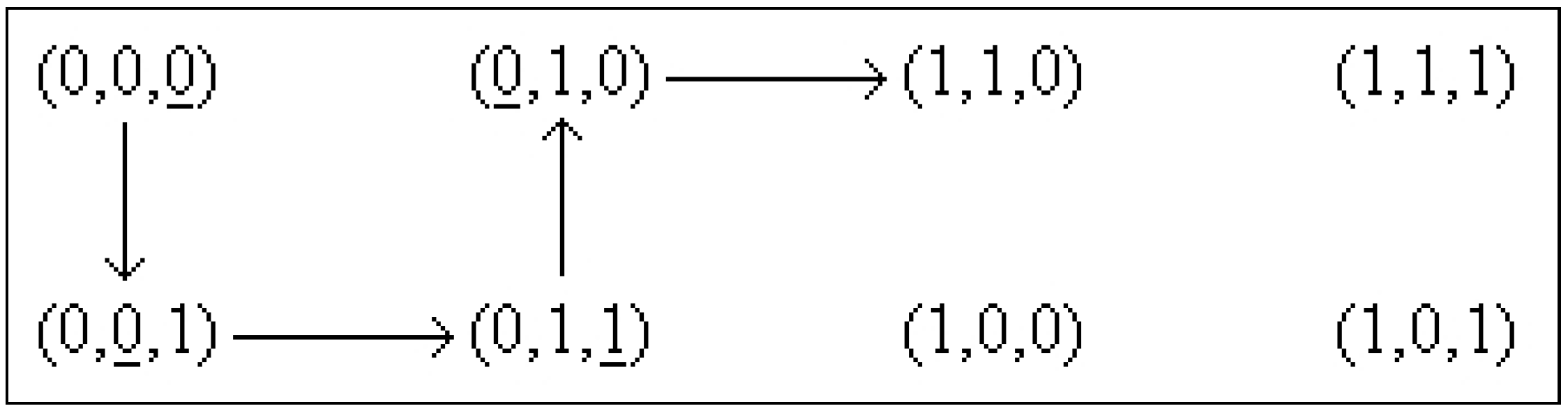
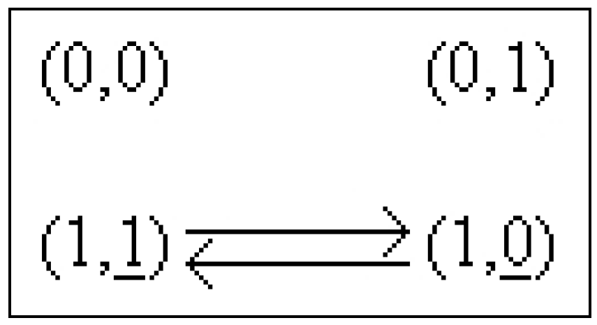
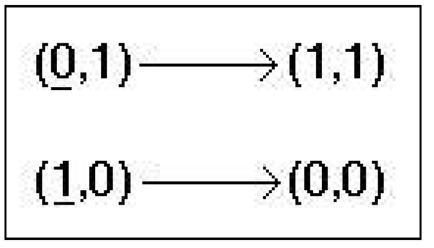
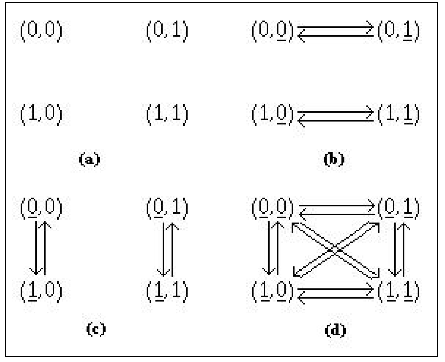
Remark 21

The fact that $(1_{{\mathbf{B}}^n},1_{{\mathbf{B}}^n})\in \overline{Aut}(\Phi )$ implies $\overline{Aut}(\Phi )\ne \varnothing ,$ but all of $\overline{Iso}(\Phi ,\mathrm{\Psi }){,}^{*}\overline{Iso}(\Phi ,\mathrm{\Psi })$ and ${}^{*}\overline{Aut}(\Phi )$ may be empty.

Definition 22

Let $\Phi ,\mathrm{\Psi }:{\mathbf{B}}^n\to {\mathbf{B}}^n,$ $\Phi \ne \mathrm{\Psi }.$ If $\overline{Iso}(\Phi ,\mathrm{\Psi })\ne \varnothing$, then ${\widehat{\overline{\Xi }}}_{\Phi },$ ${\widehat{\overline{\Xi }}}_{\mathrm{\Psi }};$ ${\overline{\Xi }}_{\Phi },{\overline{\Xi }}_{\mathrm{\Psi }};$ $\Phi ,\mathrm{\Psi }$ are called symmetrical, or conjugated; if ${}^{*}\overline{Iso}(\Phi ,\mathrm{\Psi })\ne \varnothing$, then ${\widehat{\overline{\Xi }}}_{\Phi },$ ${}^{*}{\widehat{\overline{\Xi }}}_{\mathrm{\Psi }};$ ${\overline{\Xi }}_{\Phi }{,}^{*}{\overline{\Xi }}_{\mathrm{\Psi }};$ $\Phi ,\mathrm{\Psi }$ are called anti-symmetrical, or anti-conjugated.

If $card(\overline{Aut}(\Phi ))>1,$ then ${\widehat{\overline{\Xi }}}_{\Phi },$ ${\overline{\Xi }}_{\Phi }$ and Φ are called symmetrical and if ${}^{*}\overline{Aut}(\Phi )\ne \varnothing ,$ then ${\widehat{\overline{\Xi }}}_{\Phi },$ ${\overline{\Xi }}_{\Phi }$ and Φ are called anti-symmetrical.

Remark 23

The symmetry of $\Phi ,\mathrm{\Psi }$ means that $(g,g^{\prime })\in \overline{Iso}(\Phi ,\mathrm{\Psi })$ maps the transfers $\mu \to {\Phi }^{\nu }(\mu )$ in transfers $g(\mu )\to g({\Phi }^{\nu }(\mu ))={\mathrm{\Psi }}^{g^{\prime }(\nu )}(g(\mu ));$ the situation when Φ is symmetrical and $(g,g^{\prime })\in \overline{Aut}(\Phi )$ is similar. Anti-symmetry may be understood as mirroring: $(g,g^{\prime })\in$ ${}^{*}\overline{Iso}(\Phi ,\mathrm{\Psi })$ maps the transfers (or arrows) $\mu \to {\Phi }^{\nu }(\mu )$ in transfers $g(\mu )⟵g({\Phi }^{\nu }(\mu ))={\mathrm{\Psi }}^{g^{\prime }(\nu )}(g(\mu ))$ and similarly for $(g,g^{\prime })\in$ ${}^{*}\overline{Aut}(\Phi ).$

Theorem 24

Let $\Phi ,\mathrm{\Psi }:{\mathbf{B}}^n\to {\mathbf{B}}^n.$

(a) If $(g,g^{\prime })\in \overline{Iso}(\Phi ,\mathrm{\Psi })$, then $(g^{-1},g^{\prime -1})\in \overline{Iso}(\mathrm{\Psi },\Phi ).$

(b) If $(g,g^{\prime })\in$${}^{*}\overline{Iso}(\Phi ,\mathrm{\Psi })$, then $(g^{-1},g^{\prime -1})\in$ ${}^{*}\overline{Iso}(\mathrm{\Psi },\Phi ).$

Proof. 

(a): The hypothesis states that $\forall \nu \in {\mathbf{B}}^n,$ the diagram

$$\begin{array}{ccc}{\mathbf{B}}^n& \stackrel{{\Phi }^{\nu }}{\to }& {\mathbf{B}}^n\\ g\downarrow & & \downarrow g\\ {\mathbf{B}}^n& \stackrel{{\mathrm{\Psi }}^{g^{\prime }(\nu )}}{\to }& {\mathbf{B}}^n\end{array}$$

commutes, with $g,g^{\prime }$ bijective. We fix arbitrarily $\nu \in {\mathbf{B}}^n,\mu \in {\mathbf{B}}^n.$ We denote ${\mu }^{\prime }=g(\mu ),{\nu }^{\prime }=g^{\prime }(\nu )$ and we note that

$$g^{-1}({\mathrm{\Psi }}^{{\nu }^{\prime }}({\mu }^{\prime }))={\Phi }^{g^{\prime -1}({\nu }^{\prime })}(g^{-1}({\mu }^{\prime }))$$

(9)

As $\nu ,\mu$ were chosen arbitrarily and on the other hand, when $\nu$ runs in ${\mathbf{B}}^n,{\nu }^{\prime }$ runs in ${\mathbf{B}}^n$ and when $\mu$ runs in ${\mathbf{B}}^n,{\mu }^{\prime }$ runs in ${\mathbf{B}}^n$, we infer that Equation (9) is equivalent with the commutativity of the diagram

$$\begin{array}{ccc}{\mathbf{B}}^n& \stackrel{{\mathrm{\Psi }}^{{\nu }^{\prime }}}{\to }& {\mathbf{B}}^n\\ g^{-1}\downarrow & & \downarrow g^{-1}\\ {\mathbf{B}}^n& \stackrel{{\Phi }^{g^{{}^{\prime }-1}({\nu }^{\prime })}}{\to }& {\mathbf{B}}^n\end{array}$$

for any ${\nu }^{\prime }\in {\mathbf{B}}^n.$ We have proved that $(g^{-1},g^{{}^{\prime }-1})\in \overline{Iso}(\mathrm{\Psi },\Phi ).$

(b): By hypothesis $\forall \nu \in {\mathbf{B}}^n$, the diagram

$$\begin{array}{ccc}{\mathbf{B}}^n& \stackrel{{\Phi }^{\nu }}{\to }& {\mathbf{B}}^n\\ g\downarrow & & \downarrow g\\ {\mathbf{B}}^n& \stackrel{{\mathrm{\Psi }}^{g^{\prime }(\nu )}}{⟵}& {\mathbf{B}}^n\end{array}$$

is commutative, $g,g^{\prime }$ bijective and we prove that $\forall {\nu }^{\prime }\in {\mathbf{B}}^n$, the diagram

$$\begin{array}{ccc}{\mathbf{B}}^n& \stackrel{{\mathrm{\Psi }}^{{\nu }^{\prime }}}{\to }& {\mathbf{B}}^n\\ g^{-1}\downarrow & & \downarrow g^{-1}\\ {\mathbf{B}}^n& \stackrel{{\Phi }^{g^{{}^{\prime }-1}({\nu }^{\prime })}}{⟵}& {\mathbf{B}}^n\end{array}$$

is commutative.

Theorem 25

$\overline{Aut}(\Phi )$ is a group relative to the law: $\forall (g,g^{\prime })\in \overline{Aut}(\Phi ),$ $\forall (h,h^{\prime })\in \overline{Aut}(\Phi ),$

$$(h,h^{\prime })\circ (g,g^{\prime })=(h\circ g,h^{\prime }\circ g^{\prime })$$

Proof. 

The fact that $\forall (g,g^{\prime })\in \overline{Aut}(\Phi ),\forall (h,h^{\prime })\in \overline{Aut}(\Phi ),(h\circ g,h^{\prime }\circ g^{\prime })\in \overline{Aut}(\Phi )$ is proved like this: $\forall \nu \in {\mathbf{B}}^n,$

$$\begin{array}{cc}\hfill (h\circ g)\circ {\Phi }^{\nu }& =h\circ (g\circ {\Phi }^{\nu })=h\circ ({\Phi }^{g^{\prime }(\nu )}\circ g)=(h\circ {\Phi }^{g^{\prime }(\nu )})\circ g\hfill \\ & =({\Phi }^{h^{\prime }(g^{\prime }(\nu ))}\circ h)\circ g={\Phi }^{(h^{\prime }\circ g^{\prime })(\nu )}\circ (h\circ g)\hfill \end{array}$$

the fact that $(1_{{\mathbf{B}}^n},1_{{\mathbf{B}}^n})\in \overline{Aut}(\Phi )$ was mentioned before; and the fact that $\forall (g,g^{\prime })\in \overline{Aut}(\Phi ),$ $(g^{-1},g^{{}^{\prime }-1})\in \overline{Aut}(\Phi )$ was shown at Theorem 24(a).

Definition 26

Any subgroup $G\subset \overline{Aut}(\Phi )$ with $card(G)>1$ is called a group of symmetry of ${\widehat{\overline{\Xi }}}_{\Phi },$ of ${\overline{\Xi }}_{\Phi }$ or of $\Phi .$

6. Examples

Example 27

$\Phi ,\mathrm{\Psi }:{\mathbf{B}}^2\to {\mathbf{B}}^2$ are given by, see Figure 4

$$\begin{array}{cc}\hfill \forall ({\mu }_1,{\mu }_2)\in {\mathbf{B}}^2,\Phi ({\mu }_1,{\mu }_2)& =({\mu }_1\oplus {\mu }_2,\overline{{\mu }_2})\hfill \\ \hfill \forall ({\mu }_1,{\mu }_2)\in {\mathbf{B}}^2,\mathrm{\Psi }({\mu }_1,{\mu }_2)& =(\overline{{\mu }_1},\overline{{\mu }_1}\overline{{\mu }_2}\cup {\mu }_1{\mu }_2)\hfill \end{array}$$

and the bijections $g,g^{\prime }:{\mathbf{B}}^2\to {\mathbf{B}}^2$ are $\forall ({\mu }_1,{\mu }_2)\in {\mathbf{B}}^2,$

$$\begin{array}{cc}\hfill g({\mu }_1,{\mu }_2)& =(\overline{{\mu }_2},\overline{{\mu }_1})\hfill \\ \hfill g^{\prime }({\mu }_1,{\mu }_2)& =({\mu }_2,{\mu }_1)\hfill \end{array}$$

(in order to understand the choice of $g^{\prime },$ to be remarked in Figure 4 the positions of the underlined coordinates for Φ and Ψ). Φ and Ψ are conjugated.

Example 28

The system from Figure 5 is symmetrical and a group of symmetry is generated by the couples $(g,1_{{\mathbf{B}}^3}),(u,1_{{\mathbf{B}}^3}),(v,1_{{\mathbf{B}}^3}),$ see Equation (10); $g,u,v$ are transpositions that permute the isolated fixed points $(1,0,0),(1,0,1),(1,1,1).$

$$\begin{array}{c}\begin{array}{ccccc}({\mu }_1,{\mu }_2,{\mu }_3)& 1_{{\mathbf{B}}^3}& g& u& v\\ (0,0,0)& (0,0,0)& (0,0,0)& (0,0,0)& (0,0,0)\\ (0,0,1)& (0,0,1)& (0,0,1)& (0,0,1)& (0,0,1)\\ (0,1,0)& (0,1,0)& (0,1,0)& (0,1,0)& (0,1,0)\\ (0,1,1)& (0,1,1)& (0,1,1)& (0,1,1)& (0,1,1)\\ (1,0,0)& (1,0,0)& (1,0,0)& (1,0,1)& (1,1,1)\\ (1,0,1)& (1,0,1)& (1,1,1)& (1,0,0)& (1,0,1)\\ (1,1,0)& (1,1,0)& (1,1,0)& (1,1,0)& (1,1,0)\\ (1,1,1)& (1,1,1)& (1,0,1)& (1,1,1)& (1,0,0)\end{array}\hfill \end{array}$$

(10)

Example 29

The function $\Phi :{\mathbf{B}}^2\to {\mathbf{B}}^2$ defined by $\forall \mu \in {\mathbf{B}}^2,\Phi ({\mu }_1,{\mu }_2)=(\overline{{\mu }_1},\overline{{\mu }_2})$ fulfills for $\nu \in {\mathbf{B}}^2:$

$$\begin{array}{cc}\hfill {\Phi }^{\nu }({\mu }_1,{\mu }_2)& =(\overline{{\nu }_1}{\mu }_1\oplus {\nu }_1\overline{{\mu }_1},\overline{{\nu }_2}{\mu }_2\oplus {\nu }_2\overline{{\mu }_2})\hfill \\ \hfill ({\Phi }^{\nu }\circ {\Phi }^{\nu })({\mu }_1,{\mu }_2)& =(\overline{{\nu }_1}{\Phi }_1^{{\nu }_1}({\mu }_1,{\mu }_2)\oplus {\nu }_1\overline{{\Phi }_1^{{\nu }_1}({\mu }_1,{\mu }_2)}),\overline{{\nu }_2}{\Phi }_2^{{\nu }_2}({\mu }_1,{\mu }_2)\oplus {\nu }_2\overline{{\Phi }_2^{{\nu }_2}({\mu }_1,{\mu }_2)})\hfill \\ & =(\overline{{\nu }_1}(\overline{{\nu }_1}{\mu }_1\oplus {\nu }_1\overline{{\mu }_1})\oplus {\nu }_1(\overline{{\nu }_1}{\mu }_1\oplus {\nu }_1\overline{{\mu }_1}\oplus 1),\overline{{\nu }_2}(\overline{{\nu }_2}{\mu }_2\oplus {\nu }_2\overline{{\mu }_2})\oplus {\nu }_2(\overline{{\nu }_2}{\mu }_2\oplus {\nu }_2\overline{{\mu }_2}\oplus 1))\hfill \\ & =(({\nu }_1\oplus 1){\mu }_1\oplus {\nu }_1({\mu }_1\oplus 1)\oplus {\nu }_1,({\nu }_2\oplus 1){\mu }_2\oplus {\nu }_2({\mu }_2\oplus 1)\oplus {\nu }_2)\hfill \\ & =({\nu }_1{\mu }_1\oplus {\mu }_1\oplus {\nu }_1{\mu }_1\oplus {\nu }_1\oplus {\nu }_1,{\nu }_2{\mu }_2\oplus {\mu }_2\oplus {\nu }_2{\mu }_2\oplus {\nu }_2\oplus {\nu }_2)\hfill \\ & =({\mu }_1,{\mu }_2)\hfill \end{array}$$

thus $(1_{{\mathbf{B}}^2},1_{{\mathbf{B}}^2})\in$ ${}^{*}\overline{Aut}(\Phi )$ and Φ is anti-symmetrical. The state portrait of Φ was drawn in Figure 1(c).

Notation 30

Let $\sigma :\{1,\dots ,n\}\to \{1,\dots ,n\}$ be a bijection. We use the notation ${\pi }_{\sigma }:{\mathbf{B}}^n\to {\mathbf{B}}^n$ for the bijection given by $\forall \mu \in {\mathbf{B}}^n,$

$${\pi }_{\sigma }({\mu }_1,\dots ,{\mu }_n)=({\mu }_{\sigma (1)},\dots ,{\mu }_{\sigma (n)})$$

Definition 31

Any of ${\widehat{\overline{\Xi }}}_{\Phi },$ ${\overline{\Xi }}_{\Phi }$ and $\Phi :{\mathbf{B}}^n\to {\mathbf{B}}^n$ is called symmetrical relative to the coordinates if the bijection σ exists, $\sigma \ne 1_{\{1,\dots ,n\}}$ such that $({\pi }_{\sigma },{\pi }_{\sigma })\in \overline{Aut}(\Phi ).$

Example 32

We consider the function $\Phi :{\mathbf{B}}^3\to {\mathbf{B}}^3$ defined by $\forall \mu \in {\mathbf{B}}^3,$ $\Phi ({\mu }_1,{\mu }_2,{\mu }_3)=({\mu }_2{\mu }_3\oplus {\mu }_1\oplus {\mu }_2,{\mu }_1{\mu }_3\oplus {\mu }_2\oplus {\mu }_3,{\mu }_1{\mu }_2\oplus {\mu }_1\oplus {\mu }_3)$ and the permutation $\sigma :\{1,2,3\}\to \{1,2,3\},$ $\sigma =\left(\begin{array}{ccc}1& 2& 3\\ \sigma (1)& \sigma (2)& \sigma (3)\end{array}\right)=\left(\begin{array}{ccc}1& 2& 3\\ 3& 1& 2\end{array}\right).$ A group of symmetry of ${\overline{\Xi }}_{\Phi }$ is represented by $G=\{(1_{{\mathbf{B}}^3},1_{{\mathbf{B}}^3}),$ $({\pi }_{\sigma },{\pi }_{\sigma }),({\pi }_{\sigma \circ \sigma },{\pi }_{\sigma \circ \sigma })\}.$ We have given in Figure 6 the state portrait of $\Phi .$

Notation 33

For $\lambda \in {\mathbf{B}}^n,$ we denote by ${\theta }^{\lambda }:{\mathbf{B}}^n\to {\mathbf{B}}^n$ the translation of vector $\lambda :$ $\forall \mu \in {\mathbf{B}}^n,$

$${\theta }^{\lambda }(\mu )=\mu \oplus \lambda$$

Definition 34

If $({\theta }^{\lambda },g^{\prime })\in \overline{Aut}(\Phi )$ holds for some $({\theta }^{\lambda },g^{\prime })\ne (1_{{\mathbf{B}}^n},1_{{\mathbf{B}}^n})$, we say that any of ${\widehat{\overline{\Xi }}}_{\Phi },$ ${\overline{\Xi }}_{\Phi }$ and Φ is symmetrical relative to translations.

Example 35

In Figure 7

we have the system with Φ given by Equation (11)

$$\begin{array}{c}\begin{array}{cc}({\mu }_1,{\mu }_2,{\mu }_3)& \Phi \\ (0,0,0)& (0,0,0)\\ (0,0,1)& (0,0,1)\\ (0,1,0)& (0,1,1)\\ (0,1,1)& (0,1,0)\\ (1,0,0)& (0,1,1)\\ (1,0,1)& (0,1,0)\\ (1,1,0)& (1,0,0)\\ (1,1,1)& (1,0,1)\end{array}\hfill \end{array}$$

(11)

and $({\theta }^{(0,0,1)},1_{{\mathbf{B}}^3})\in \overline{Aut}(\Phi ),$ as resulting from the state portrait.

Example 36

In Equation (12) we have a function $\Phi :{\mathbf{B}}^2\to {\mathbf{B}}^2$ for which four functions $g_1^{\prime },g_2^{\prime },g_3^{\prime },g_4^{\prime }:{\mathbf{B}}^2\to {\mathbf{B}}^2$ exist:

$$\begin{array}{c}\begin{array}{cccccc}({\mu }_1,{\mu }_2)& \Phi & g_1^{\prime }& g_2^{\prime }& g_3^{\prime }& g_4^{\prime }\\ (0,0)& (0,0)& (0,0)& (1,0)& (0,0)& (1,0)\\ (0,1)& (0,1)& (0,1)& (0,1)& (1,1)& (1,1)\\ (1,0)& (1,1)& (1,0)& (0,0)& (1,0)& (0,0)\\ (1,1)& (1,0)& (1,1)& (1,1)& (0,1)& (0,1)\end{array}\hfill \end{array}$$

(12)

such that $(1_{{\mathbf{B}}^2},g_1^{\prime }),(1_{{\mathbf{B}}^2},g_2^{\prime }),(1_{{\mathbf{B}}^2},g_3^{\prime }),(1_{{\mathbf{B}}^2},g_4^{\prime })\in \overline{Aut}(\Phi ).$ The state portrait of Φ is drawn Figure 8.

Example 37

The system from Figure 9 is symmetrical relative to translations, since it has the group of symmetry $G=\{(1_{{\mathbf{B}}^2},1_{{\mathbf{B}}^2}),({\theta }^{(1,1)},1_{{\mathbf{B}}^2})\}.$Φ is self-dual $\Phi ={\Phi }^{*},$ where the dual ${\Phi }^{*}$ of Φ is defined by ${\Phi }^{*}(\mu )=\overline{\Phi (\overline{\mu })}.$

Example 38

Functions $\Phi :{\mathbf{B}}^2\to {\mathbf{B}}^2$ exist, see Figure 10, that are symmetrical relative to the translations with any $\lambda \in {\mathbf{B}}^2,$ thus their group of symmetry is $G=\{(1_{{\mathbf{B}}^2},1_{{\mathbf{B}}^2}),({\theta }^{(0,1)},1_{{\mathbf{B}}^2}),({\theta }^{(1,0)},1_{{\mathbf{B}}^2}),({\theta }^{(1,1)},1_{{\mathbf{B}}^2})\}.$ The fact that $({\theta }^{(1,1)},1_{{\mathbf{B}}^2})\in G$ shows that all these functions: $\Phi (\mu )=({\mu }_1,{\mu }_2),$ $\Phi (\mu )=({\mu }_1,\overline{{\mu }_2}),$ $\Phi (\mu )=(\overline{{\mu }_1},{\mu }_2),$ $\Phi (\mu )=(\overline{{\mu }_1},\overline{{\mu }_2})$ are self-dual, $\Phi ={\Phi }^{*}.$

Example 39

The group of symmetry G of the system from Figure 11 has four elements given by Equation (13)

$$\begin{array}{c}\begin{array}{ccccc}({\mu }_1,{\mu }_2)& 1_{{\mathbf{B}}^2}& g& h& {\theta }^{(1,1)}\\ (0,0)& (0,0)& (0,1)& (1,0)& (1,1)\\ (0,1)& (0,1)& (1,1)& (0,0)& (1,0)\\ (1,0)& (1,0)& (0,0)& (1,1)& (0,1)\\ (1,1)& (1,1)& (1,0)& (0,1)& (0,0)\end{array}\hfill \end{array}$$

(13)

and we remark that $h=g^{-1},{\theta }^{(1,1)}={({\theta }^{(1,1)})}^{-1}$ hold, see also Equation (14).

$$\begin{array}{c}\begin{array}{ccccc}({\nu }_1,{\nu }_2)& {{(}_{1_{{\mathbf{B}}^2}})}^{\prime }& g^{\prime }& h^{\prime }& {({\theta }^{(1,1)})}^{\prime }\\ (0,0)& (0,0)& (0,0)& (0,0)& (0,0)\\ (0,1)& (0,1)& (1,0)& (1,0)& (0,1)\\ (1,0)& (1,0)& (0,1)& (0,1)& (1,0)\\ (1,1)& (1,1)& (1,1)& (1,1)& (1,1)\end{array}\hfill \end{array}$$

(14)

We have $\Phi ={\Phi }^{*}$ like previously.

7. Conclusions

The paper defines the universal semi-regular autonomous asynchronous systems and the universal anti-semi-regular autonomous asynchronous systems. It also defines and characterizes the isomorphisms (automorphisms) and the anti-isomorphisms (anti-automorphisms) of these systems. Symmetry is defined as the existence of such isomorphisms (automorphisms), while anti-symmetry is defined as the existence of such anti-isomorphisms (anti-automorphisms). Many examples are given. A by-pass product in this study is anti-symmetry, which is related with systems having the cause in the future and the effect in the past. Another by-pass product consists in semi-regularity, since important examples of isomorphisms (automorphisms) are of semi-regular systems only and do not keep progressiveness and regularity [2,3].

References

1. Kuznetsov, Y.A. Elements of Applied Bifurcation Theory, 2nd ed.; Springer: Berlin, Germany, 1997. [Google Scholar]
2. Vlad, S.E. Boolean dynamical systems. ROMAI J. 2007, 3, 277–324. [Google Scholar]
3. Vlad, S.E. Universal regular autonomous asynchronous systems: Fixed points, equivalencies and dynamical bifurcations. ROMAI J. 2009, 5, 131–154. [Google Scholar]
Figure 1. (a) the logical gate NOT; (b) circuit with logical gates NOT; (c) state portrait.
Symmetry 04 00116 g001
Figure 2. The semi-regular system Ξ ¯ Φ from Example 11.
Symmetry 04 00116 g002
Figure 3. The semi-regular system Ξ ¯ Ψ from Example 15.
Symmetry 04 00116 g003
Figure 4. Symmetrical systems, Example 27.
Symmetry 04 00116 g004
Figure 5. Symmetrical system, Example 28.
Symmetry 04 00116 g005
Figure 6. System that is symmetrical relative to the coordinates, Example 32.
Symmetry 04 00116 g006
Figure 7. Φ has the automorphism ( θ ( 0 , 0 , 1 ) , 1 B 3 ) , Example 35.
Symmetry 04 00116 g007
Figure 8. Φ is symmetrical relative to translations with ( 0 , 0 ) , Example 36.
Symmetry 04 00116 g008
Figure 9. Function Φ that is self dual, ( θ ( 1 , 1 ) , 1 B 2 ) A u t ¯ ( Φ ) , Example 37.
Symmetry 04 00116 g009
Figure 10. Functions Φ that are self dual, ( θ ( 1 , 1 ) , 1 B 2 ) A u t ¯ ( Φ ) , Example 38.
Symmetry 04 00116 g010
Figure 11. Symmetry including symmetry relative to translations, Example 39.
Symmetry 04 00116 g011