Lattices of Graphical Gaussian Models with Symmetries

Abstract
:1. Introduction
2. Preliminaries and Notation
2.1. Notation
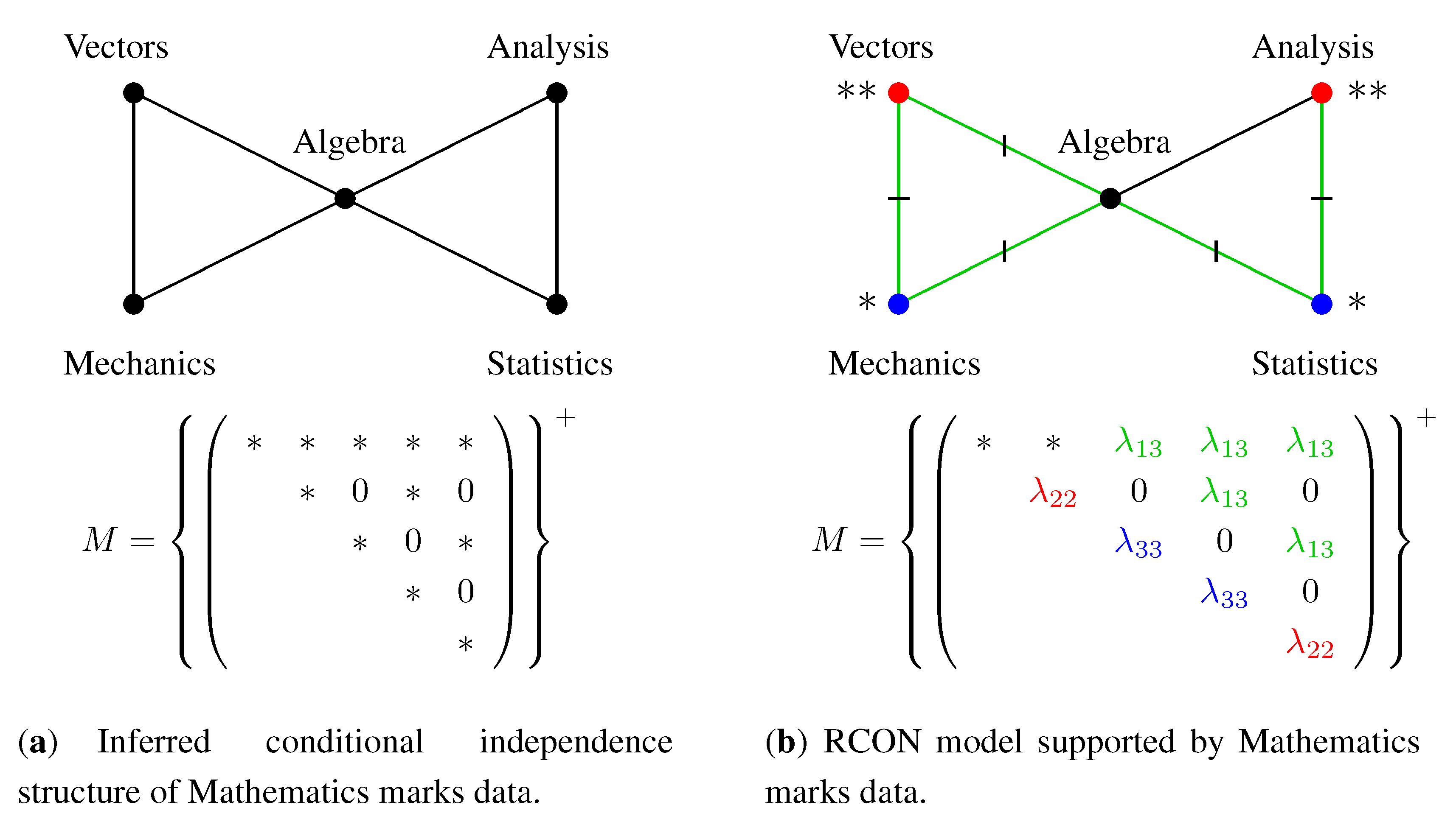
2.2. Graphical Gaussian Models
2.3. Graph Colouring
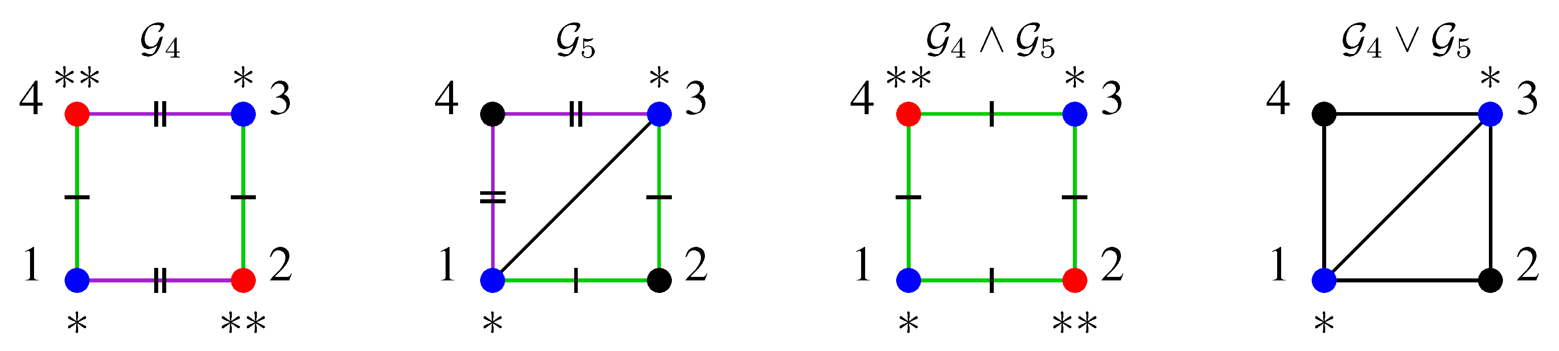
2.4. Lattices
3. Model Types: RCON and RCOR Models
3.1. RCON Models: Equality Restrictions on Concentrations
3.2. RCOR Models: Equality Restrictions on Partial Correlations
3.3. Number of RCON and RCOR Models
3.4. Structure of the Sets of RCON and RCOR Models
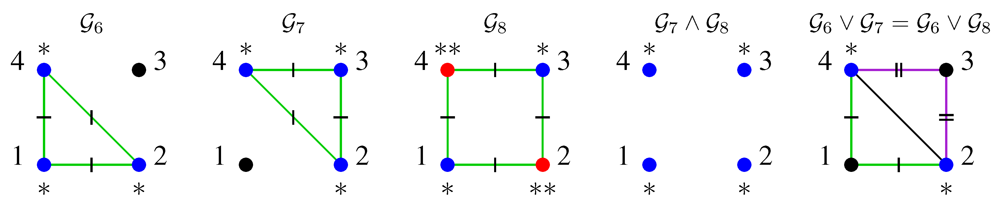
- (i)
- ; (ii) ; (iii) every edge colour class in is a union of colour classes in .
4. Model Classes within RCON and RCOR Models
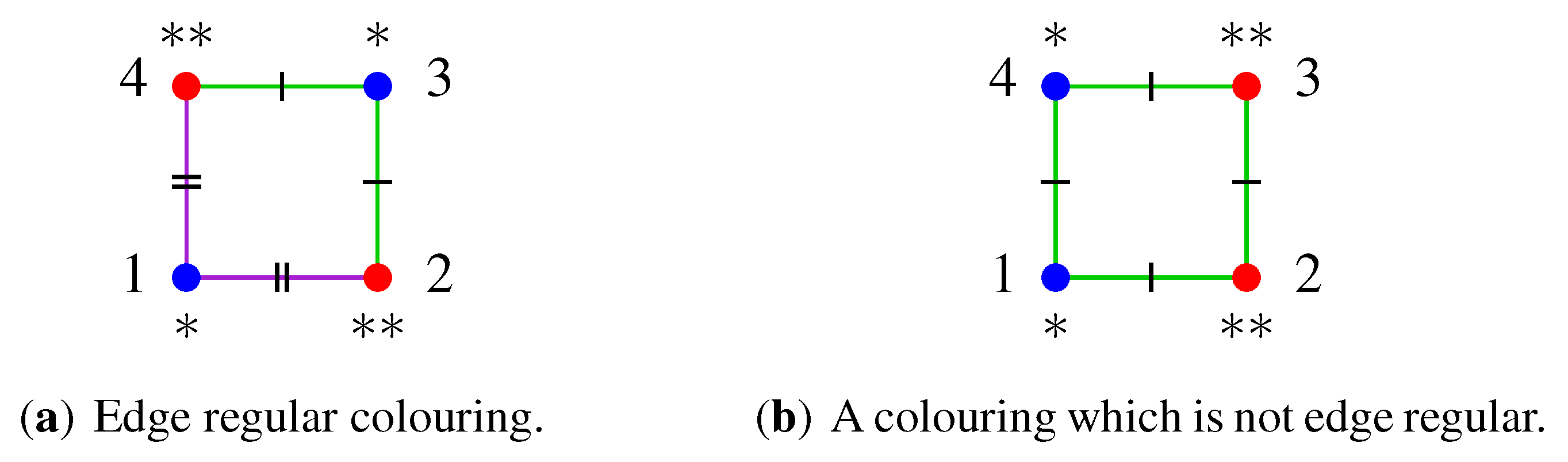
4.1. Models Represented by Edge Regular Colourings
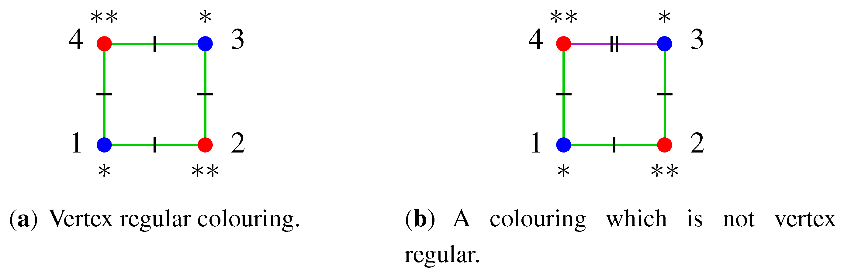
4.2. Models Represented by Vertex Regular Colourings
- (i)
- the likelihood function based on is maximised in μ by the least-squares estimator for all Σ with or with where
- (ii)
- is finer than and is vertex regular.
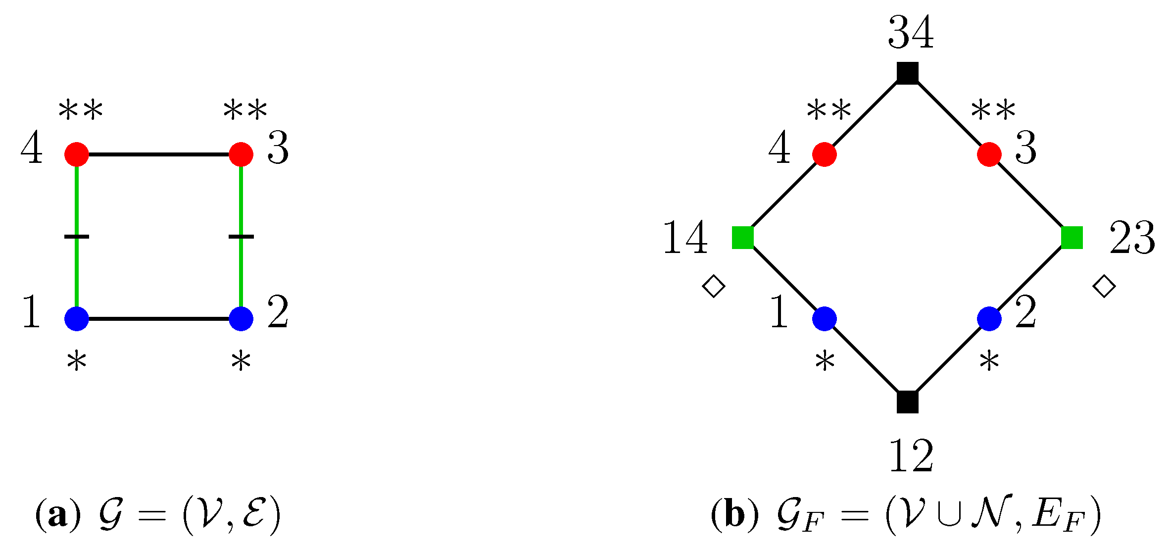
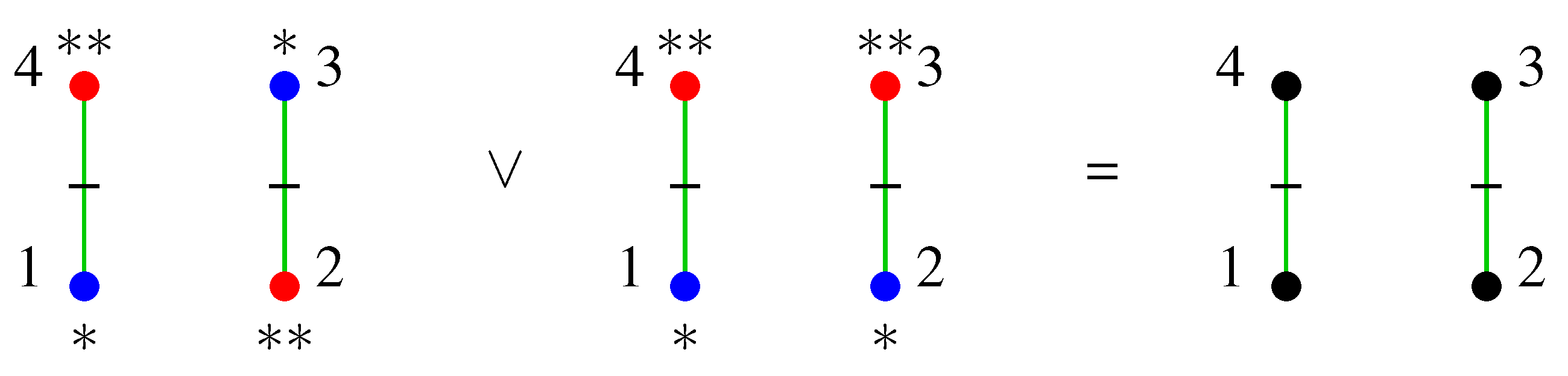
4.3. Models Represented by Regular Colourings
- (i)
- every pair of equally coloured edges in connects the same vertex colour classes in ;
- (ii)
- every pair of equally coloured vertices in has the same degree in every edge colour class in .
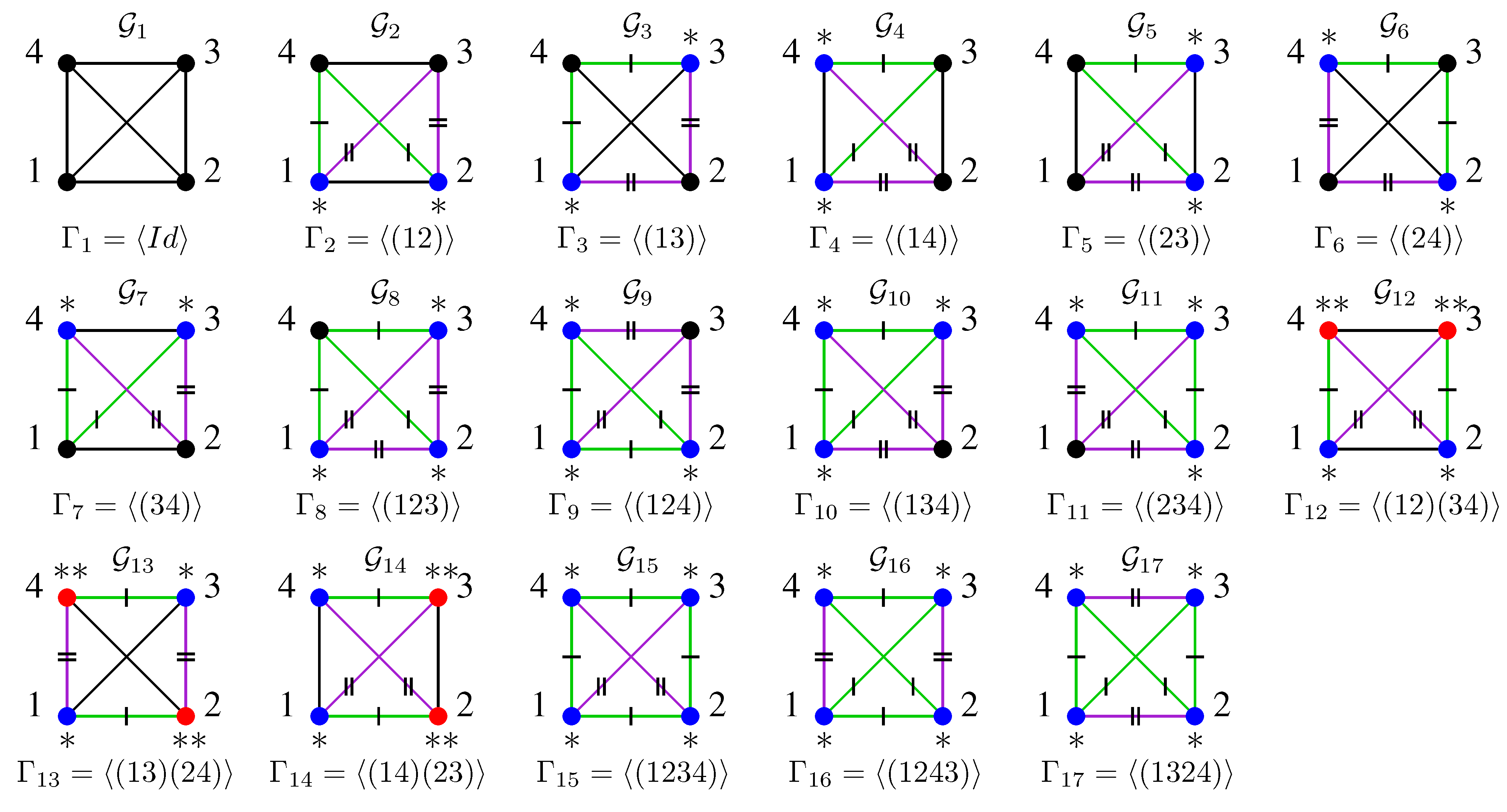
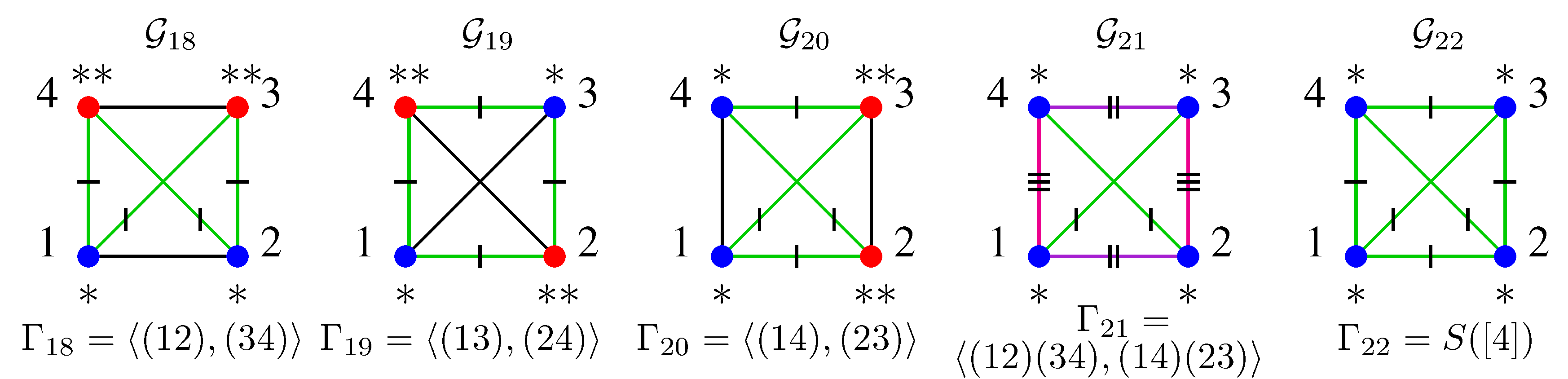
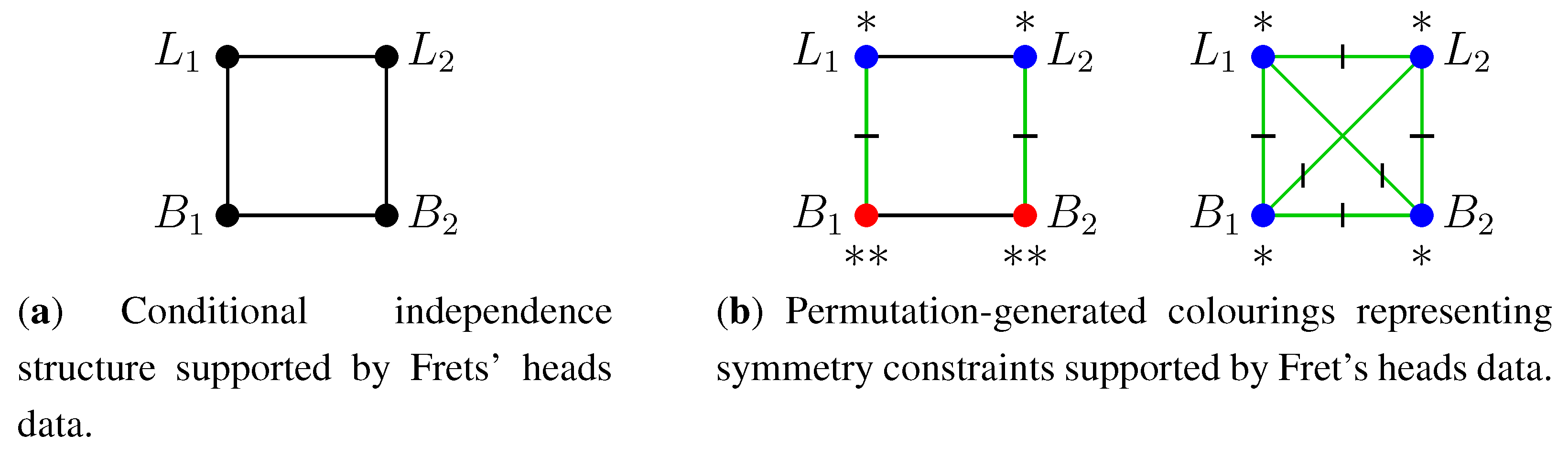
4.4. Models Represented by Permutation-Generated Colourings
4.5. Relations Between Model Classes
5. Structures of Model Classes
5.1. Models Represented by Edge Regular Colourings
5.2. Models Represented by Permutation-Generated Colourings
5.3. Models Represented by Regular and Vertex Regular Colourings
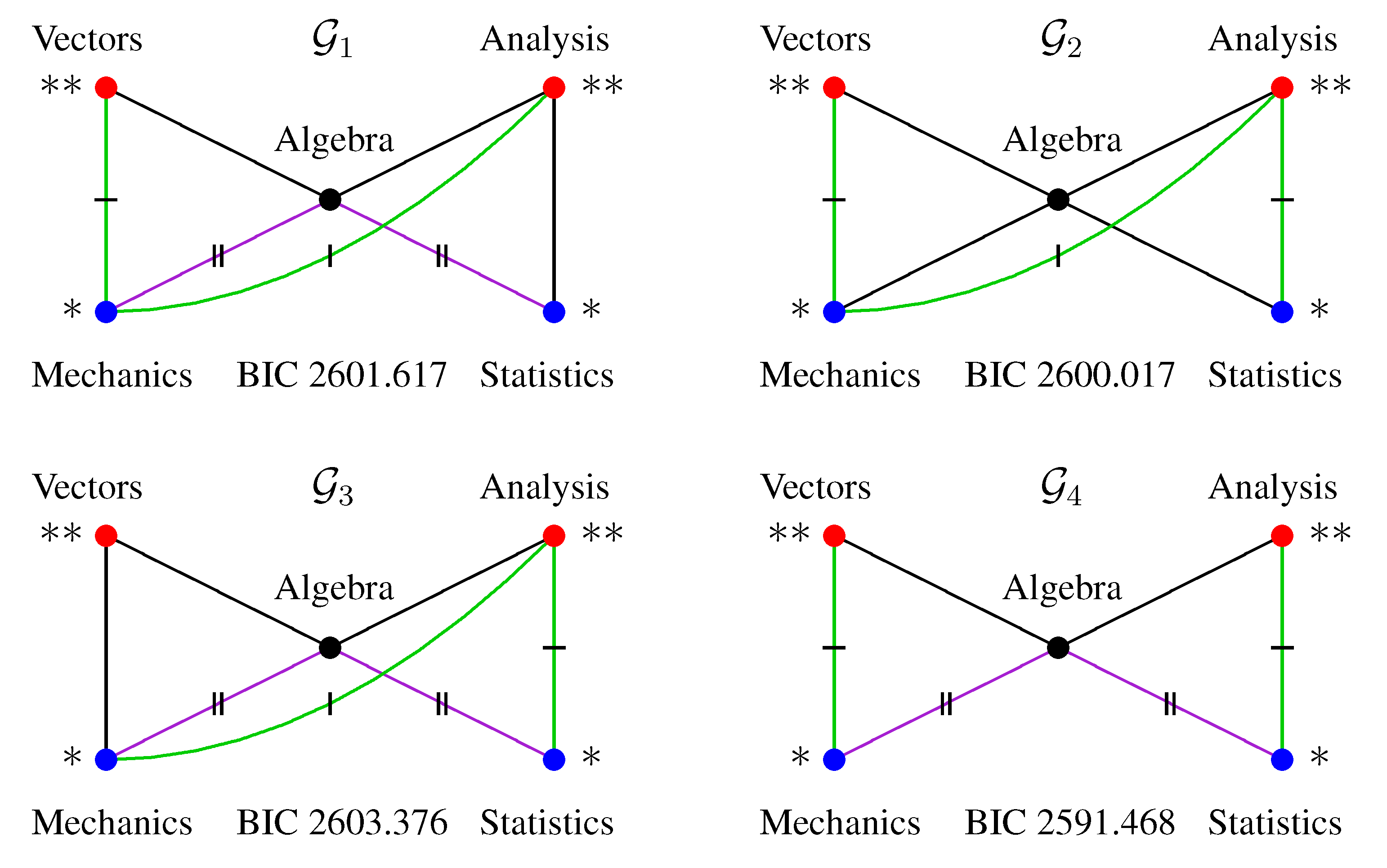
6. Model Selection
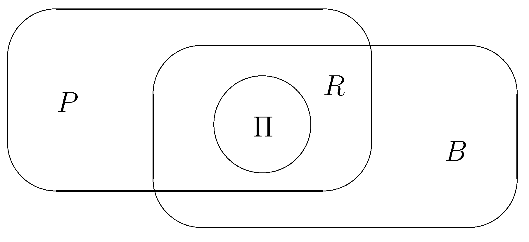
6.1. The Edwards–Havránek Model Selection Procedure
- Test an initial set of models and assign the accepted models to and the rejected models to .
- Choose between 3 and 4.
- Test the models in . If all are rejected, stop; otherwise, update and and go to 2.
- Test the models in . If all are accepted, stop; otherwise, update and and go to 2.
6.2. Models with Edge Regular Colourings
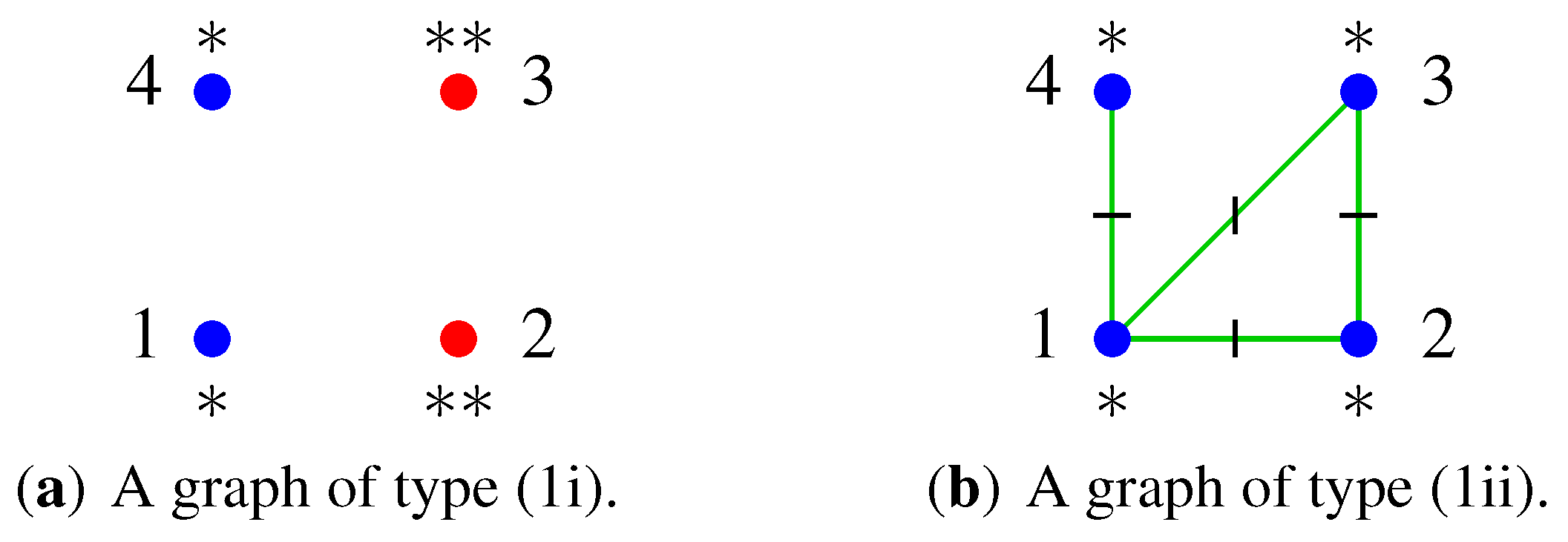
- (1i)
- such that and
- (1ii)
- and with and .
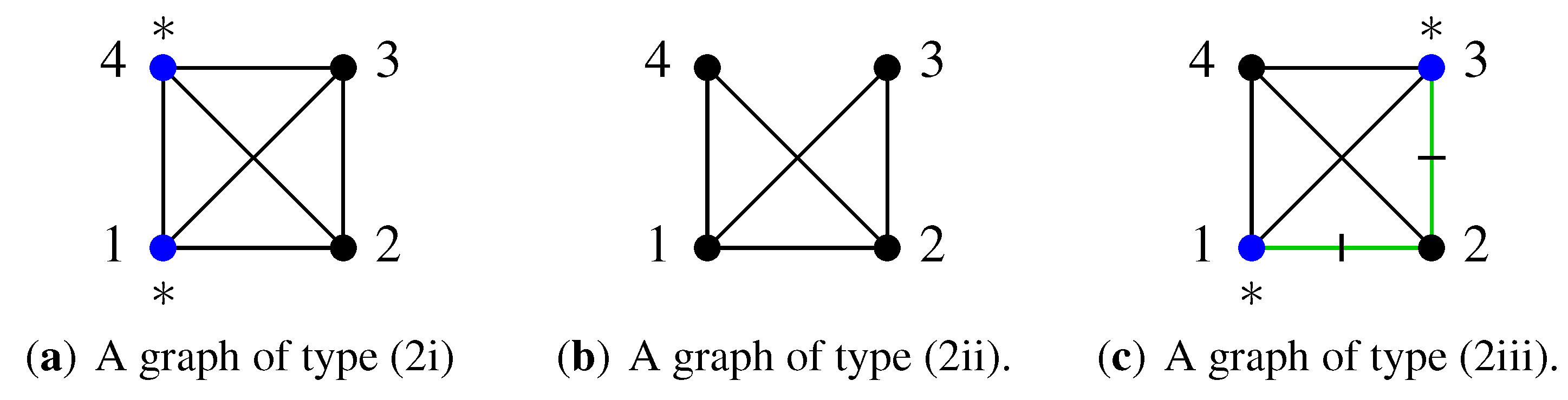
- (2i)
- such that and , or
- (2ii)
- and with , or
- (2iii)
- with and being of the same colour in and , where we may have or but not both, such that .
- Test an initial set of models and assign each to if it is rejected and to otherwise.
- Test the models in . If all are rejected, stop. Otherwise update and and repeat.
6.3. Models Represented by Permutation-Generated Colourings
7. Discussion
Acknowledgments
References
- Højsgaard, S.; Lauritzen, S.L. Graphical Gaussian models with edge and vertex symmetries. J. R. Stat. Soc. Ser. B 2008, 70, 1005–1027. [Google Scholar] [CrossRef]
- Edwards, D.; Havránek, T. A fast model selection procedure for large families of models. J. Am. Stat. Assoc. 1987, 82, 205–213. [Google Scholar] [CrossRef]
- Lauritzen, S.L. Graphical Models; Clarendon Press: Oxford, UK, 1996. [Google Scholar]
- Gottard, A.; Marchetti, G.M.; Agresti, A. Quasi-symmetric graphical log-linear models. Scand. J. Stat. 2011, 38, 447–465. [Google Scholar] [CrossRef]
- Ramírez-Aldana, R. Restricted or Coloured Graphical Log-Linear Models. PhD thesis, Graduate studies in Mathematics, National Autonomous University of Mexico, Mexico City, Mexico, 2010. [Google Scholar]
- Uhler, C. Geometry of Maximum Likelihood Estimation in Gaussian Graphical Models. 2010. Available online: http://arxiv.org/abs/1012.2643 (accessed on 2 September 2011).
- Wilks, S.S. Sample criteria for testing equality of means, equality of variances, and equality of covariances in a normal multivariate distribution. Ann. Math. Stat. 1946, 17, 257–281. [Google Scholar] [CrossRef]
- Votaw, D.F. Testing compound symmetry in a normal multivariate distribution. Ann. Math. Stat. 1948, 19, 447–473. [Google Scholar] [CrossRef]
- Olkin, I.; Press, S.J. Testing and estimation for a circular stationary model. Ann. Math. Stat. 1969, 40, 1358–1373. [Google Scholar] [CrossRef]
- Olkin, I. Testing and Estimation for Structures Which Are Circularly Symmetric in Blocks; Technical Report; Educational Testing Service: Princeton, NJ, USA, 1972. [Google Scholar]
- Andersson, S.A. Invariant normal models. Ann. Math. Stat. 1975, 3, 132–154. [Google Scholar] [CrossRef]
- Jensen, S.T. Covariance hypotheses which are linear in both the covariance and the inverse covariance. Ann. Stat. 1988, 16, 302–322. [Google Scholar] [CrossRef]
- Hylleberg, B.; Jensen, M.; Ørnbøl, E. Graphical Symmetry Models. Master’s thesis, Aalborg University, Aalborg, Denmark, 1993. [Google Scholar]
- Andersen, H.H.; Højbjerre, M.; Sørensen, D.; Eriksen, P.S. Linear and Graphical Models for the Multivariate Complex Normal Distribution; Springer Verlag: New York, NY, USA, 1995. [Google Scholar]
- Madsen, J. Invariant normal models with recursive graphical Markov structure. Ann. Stat. 2000, 28, 1150–1178. [Google Scholar] [CrossRef]
- Gehrmann, H.; Lauritzen, S. Estimation of Means on Graphical Gaussian Models with Symmetries. 2011. Available online: http://arxiv.org/abs/1101.3709 (accessed on 2 September 2011).
- Frets, G.P. Heredity of head form in man. Genetica 1921, 41, 193–400. [Google Scholar] [CrossRef]
- Mardia, K.V.; Kent, J.T.; Bibby, J.M. Multivariate Analysis; Academic Press: New York, NY, USA, 1979. [Google Scholar]
- Bollobás, B. Modern Graph Theory; Springer Verlag: New York, NY, USA, 1998. [Google Scholar]
- Grätzer, G. General Lattice Theory; Birkhäuser Verlag: Basel, Switzerland, 1998. [Google Scholar]
- Brown, L.D.; Author, T. Fundamentals of Statistical Exponential Families with Applications in Statistical Decision Theory; Gupta, S.S., Ed.; Institute of Mathematical Statistics: Hayward, CA, USA, 1986. [Google Scholar]
- Højsgaard, S.; Lauritzen, S.L. Inference in graphical Gaussian models with edge and vertex symmetries with the gRc package for R. J. Stat. Softw. 2007, 23. [Google Scholar] [CrossRef]
- Anderson, T.W. Estimation of Covariance Matrices which are Linear Combinations or Whose Inverses are Linear Combinations of Given Matrices. In Essays in Probability and Statistics; Bose, R.C., Chakravati, I.M., Mahalanobis, P.C., Rao, C.R., Smith, K.J.C., Eds.; University of North Carolina Press: Chapel Hill, NC, USA, 1970; pp. 1–24. [Google Scholar]
- Whittaker, J. Graphical Models in Applied Multivariate Statistics; Wiley: Chichester, UK, 1990. [Google Scholar]
- Edwards, D. Introduction to Graphical Modelling; Springer Verlag: New York, NY, USA, 2000. [Google Scholar]
- Cox, D.R.; Wermuth, N. Linear dependencies represented by chain graphs (with discussion). Stat. Sci. 1993, 8, 204–218, 247–277. [Google Scholar] [CrossRef]
- Bell, E.T. Exponential numbers. Am. Math. Mon. 1934, 1, 411–419. [Google Scholar] [CrossRef]
- Pitman, J. Probabilistic aspects of set partitions. Am. Math. Mon. 1997, 104, 201–209. [Google Scholar] [CrossRef]
- Dobiński, G. Summierung der Reihe ∑nm/n! für m = 1,2,3,4,5,…. Grunert Arch. (Arch. Math. Phys.) 1877, 61, 333–336. [Google Scholar]
- Complet, P. Advanced Combinatorics; D. Reidel Publishing Company: Boston, MA, USA, 1974. [Google Scholar]
- Sachs, H. Über teiler, faktoren und charakteristische polynome von graphen. Wiss. Z. Tech. Hochsch. Ilmenau 1966, 12, 7–12. [Google Scholar]
- Siemons, J. Automorphism groups of graphs. Arch. Math. 1983, 41, 379–384. [Google Scholar] [CrossRef]
- Buhl, S. On the existence of maximum likelihood estimators for graphical Gaussian models. Scand. J. Stat. 1993, 20, 263–270. [Google Scholar]
- Schmidt, R. Subgroup Lattices of Groups; de Gruyter: Berlin, Germany, 1994. [Google Scholar]
- Frey, B.; Kschischang, F.; Loelinger, H.; Wiberg, N. Factor Graphs and Algorithms. In Proceedings of the 35th Allerton Conference on Communication, Control and Computing, Allerton House, Monticello, IL, USA, 29 September–1 October 1997. [Google Scholar]
- McKay, B. Backtrack Programming and the Graph Isomorphism Problem. Master’s thesis, University of Melbourne, Parkville, VIC, Australia, 1976. [Google Scholar]
- Meinshausen, N.; Bühlmann, P. High dimensional graphs and variable selection with the lasso. Ann. Stat. 2006, 34, 1436–1462. [Google Scholar] [CrossRef]
- Meinshausen, N.; Bühlmann, P. Stability selection. J. R. Stat. Soc. Ser. B 2010, 72, 417–473. [Google Scholar] [CrossRef]
- Drton, M.; Perlman, D. A SINful Approach to Gaussian graphical model selection. J. Stat. Plan. Inference 2008, 7138, 1179–1200. [Google Scholar] [CrossRef]
- Gabriel, K.R. Simultaneous test procedures—some theory of multiple comparisons. Ann. Math. Stat. 1969, 40, 224–250. [Google Scholar] [CrossRef]
- Friedman, F.; Hastie, T.; Tibshirani, R. Sparse inverse covariance estimation with the graphical lasso. Biostatistics 2008, 9, 432–441. [Google Scholar] [CrossRef] [PubMed]
- Ravikumar, P.; Wainwright, M.J.; Raskutti, G.; Yu, B. High-Dimensional Covariance Estimation by Minimizing l1-Penalized Log-Determinant Divergence. In Proceedings of the 22nd Annual Conference on Neural Information Processing Systems (NIPS), Vancouver, BC, Canada, 8–10 December 2008. [Google Scholar]
- Tibshirani, R.; Saunders, M.; Rosset, S.; Zhu, J.; Knight, K. Sparsity and smoothness via the fused lasso. J. R. Stat. Soc. Ser. B 2005, 67, 91–108. [Google Scholar] [CrossRef]


| Model class | ||||||
| Size | 13,155 | 3065 | 1380 | 251 | 251 | 64 |
© 2011 by the author; licensee MDPI, Basel, Switzerland. This article is an open access article distributed under the terms and conditions of the Creative Commons Attribution license (http://creativecommons.org/licenses/by/3.0/.)
Share and Cite
Gehrmann, H. Lattices of Graphical Gaussian Models with Symmetries. Symmetry 2011, 3, 653-679. https://doi.org/10.3390/sym3030653
Gehrmann H. Lattices of Graphical Gaussian Models with Symmetries. Symmetry. 2011; 3(3):653-679. https://doi.org/10.3390/sym3030653
Chicago/Turabian StyleGehrmann, Helene. 2011. "Lattices of Graphical Gaussian Models with Symmetries" Symmetry 3, no. 3: 653-679. https://doi.org/10.3390/sym3030653
APA StyleGehrmann, H. (2011). Lattices of Graphical Gaussian Models with Symmetries. Symmetry, 3(3), 653-679. https://doi.org/10.3390/sym3030653