Article

Lattices of Graphical Gaussian Models with Symmetries

Department of Statistics, University of Oxford, 1 South Parks Road, Oxford OX1 3TG, UK
Symmetry 2011, 3(3), 653-679; https://doi.org/10.3390/sym3030653
Submission received: 1 April 2011 / Revised: 30 August 2011 / Accepted: 5 September 2011 / Published: 7 September 2011
(This article belongs to the Special Issue Symmetry in Probability and Inference)

Abstract

:
In order to make graphical Gaussian models a viable modelling tool when the number of variables outgrows the number of observations, [1] introduced model classes which place equality restrictions on concentrations or partial correlations. The models can be represented by vertex and edge coloured graphs. The need for model selection methods makes it imperative to understand the structure of model classes. We identify four model classes that form complete lattices of models with respect to model inclusion, which qualifies them for an Edwards–Havránek model selection procedure [2]. Two classes turn out most suitable for a corresponding model search. We obtain an explicit search algorithm for one of them and provide a model search example for the other.

1. Introduction

Graphical models are probabilistic models which use graphs to represent dependencies between random variables. This article is concerned with models represented by undirected graphs, in which each variable corresponds to a vertex and a pair of vertices is joined by an edge unless the corresponding variables are conditionally independent given the remaining variables. In addition to providing a concise form of visualisation of the conditional independence structure of a model, the graphical representation can be exploited to make statistical inference computations more efficient [3].
Motivated by the growing need for parsimonious models in modern day applications, in particular when the number of variables outgrows the number of observations, in recent years graphical models with additional equality constraints on model parameters are becoming of increasing interest, in discrete models [4,5] as well as in multivariate Gaussian models, which are the central object of interest in this article. First studies [1,6] show that equality constraints reduce the minimal number of observations required to ensure estimability of the model parameters with probability one, which makes graphical Gaussian models with equality constraints a promising model class.
Symmetry constraints, induced by distribution invariance under a permutation group applied to the variable labels, are a special instance of equality constraints and have a long history for the Gaussian distribution before the advent of graphical models [7,8,9,10,11,12]. First studies of models combining symmetry constraints with conditional independence relations are given in [13,14,15]. The models we study have been introduced in [1] and contain the models in [13] and [14] as special cases. The types of restrictions are: equality between specified elements of the concentration matrix (RCON) and equality between specified partial correlations (RCOR). The models can be represented by vertex and edge coloured graphs, where parameters associated with equally coloured vertices or edges are restricted to being identical.
In order for RCON and RCOR models to become widely applicable in practice model selection methods need to be developed, which motivates the study of model structures. This is the main objective of this article. As both model types RCON and RCOR models form complete lattices, both qualify for the Edwards–Havránek model selection procedure for lattices [2]. However due to the large number of models it is more feasible to search, at least initially, in suitable subsets of the model space. Particularly favourable are subsets of models in which equality constraints are placed in a pattern which makes them more readily interpretable.
Four model classes with desirable statistical properties which express themselves in regularity of graph colouring have been previously identified in the literature: The most restrictive is given by graphical symmetry models studied in [13], also appearing in [1] under the name RCOP models. The corresponding graph colourings are given by vertex and edge orbits of a permutation group acting on the variable labels and we therefore term them permutation-generated. Colourings representing models which place the same equality constraints on the concentrations and partial correlations were termed edge regular in [16]. Two further model types, ensuring estimability of a non-zero model mean subject to equality constraints, were introduced in [16], the colourings representing them termed vertex regular and regular respectively.
The main results presented in this article are that each of the model classes forms a complete lattice of models and the identification of their meet and join operations. The former is established by showing that each model class is stable under model intersection, which gives the shared meet operation, and by demonstrating that whenever a model does not fall inside a given class there is a unique smallest larger model, or supremum, which does, giving the distinct join operations. The found lattice structure qualifies each model class for an Edwards–Havránek model search, giving a first model selection procedure for RCON and RCOR models.
We focus on models represented by edge regular and permutation-generated colourings as their structure is generally more tractable and their constraints more readily interpretable. We present an Edwards–Havránek model selection algorithm for models with edge regular colourings and illustrate it by means of an example with five variables, with a very encouraging performance. We further provide an example of a model search within models with permutation-generated colourings with four variables, commonly known as Fret’s heads [17,18].

2. Preliminaries and Notation

2.1. Notation

Let G = ( V , E ) be an undirected uncoloured graph with vertex set V and edge set E. For a | V | × | V | matrix A = ( a α β ) , A ( G ) shall denote the matrix defined by A ( G ) α β = 0 whenever there is no edge between α and β in G for α β , and A ( G ) α β = a α β otherwise. For a set of matrices M we let M + denote the set of positive-definite matrices inside M. S shall denote the set of symmetric matrices, so that S + denotes the set of symmetric positive definite matrices and S + ( G ) the set of symmetric positive definite matrices indexed by V whose α β -entry is zero for α β E for α β . We indicate that a matrix is symmetric by only writing its elements on the diagonal and above. Asterisks as matrix entries indicate that the corresponding entry is unconstrained apart from any restrictions stated explicitly.
For a discrete set D we let S ( D ) denote the set symmetric group acting on D, consisting of all permutations of the elements in D. For F S ( D ) , F denotes the group generated by F, containing all permutation which can be expressed as products of elements in F and their inverses. Permutations are written in cycle notation, meaning that σ = ( i 1 i 2 i r ) maps i j to i j + 1 for 1 j < r and i r to i 1 .
For a graph G = ( V , E ) , Aut ( G ) denotes the automorphism group of G, containing all permutations in S ( V ) which leave G invariant. For a partition P of a set S and a , b S we write a b ( P ) to denote that a and b lie in the same set in P. For n N , we denote sets of the form { 1 , 2 , , n } by [ n ] .

2.2. Graphical Gaussian Models

A graphical Gaussian model is concerned with the distribution of a multivariate random vector Y = ( Y α ) α V . Let G = ( V , E ) be an undirected graph with vertex set V and edge set E. Then the graphical Gaussian model represented by G is given by assuming that Y follows a multivariate Gaussian N | V | ( μ , Σ ) distribution with concentration matrix K = Σ 1 S + ( G ) .
The entries in K = ( k α β ) α , β V have a simple interpretation. The diagonal elements k α α are reciprocals of the conditional variances given the remaining variables
k α α = Var ( Y α | Y V { α } ) 1
for α V . The scaled elements of the concentration matrix
c α β = k α β k α α k β β
for α , β V are the negative partial correlation coefficients
ρ α β | V { α , β } = Cov ( Y α , Y β | Y V { α , β } ) Var ( Y α | Y V { α } ) 1 / 2 Var ( Y β | Y V { β } ) 1 / 2 = c α β
for α , β V . It follows that
α β E k α β = 0 Y α Y β Y V { α , β }
see e.g., Chapter 5 in [3] for further details.

2.3. Graph Colouring

For general graph terminology we refer to [19]. Following [1], for G = ( V , E ) an undirected graph, a vertex colouring of G is a partition V = { V 1 , , V k } of V, where we refer to V 1 , , V k as the vertex colour classes. Similarly, an edge colouring of G is a partition E = { E 1 , , E l } of E into ledge colour classes E 1 , , E l . A colour class with a single element is atomic and a colour class which is not atomic is composite. We let G = ( V , E ) denote the coloured graph with vertex colouring V and edge colouring E and let ( V , E ) denote its graph colouring. For V and E as above and u V , we let T u denote the | V | × | V | diagonal matrix with T α α u = 1 if and only if α u and zero otherwise. Similarly for u E , we let T u be the symmetric | V | × | V | matrix with T α β u = 1 if and only if α β u and zero otherwise.
In our display of vertex and edge coloured graphs, we indicate the colour class of a vertex by the number of asterisks we place next to it. Similarly we indicate the colour class of an edge by dashes. Vertices and edges which are displayed in black correspond to atomic colour classes.

2.4. Lattices

A binary relation ρ on a set A is a subset of A × A with two elements a , b A being in relation with respect to ρ if and only if ( a , b ) ρ , which we denote by a ρ b . If ρ is reflexive [ a ρ a a A ], antisymmetric [ a ρ b and b ρ a a = b a , b A ] and transitive [ a ρ b and b ρ c a ρ c a , b , c A ], it is a partial ordering relation and A a partially ordered set or poset. We denote a poset A with partial ordering relation ρ by A ; ρ , abbreviated by simply A if the binary relation is clear.
For H A and a A , a is an upper bound of H if h a for all h H . a is the least upper bound or supremum of H if every upper bound b of H satisfies a b and we then write a = sup H . Lower bound and greatest lower bound or infimum, denoted inf H , are defined similarly. sup is the smallest element in A, called z e r o , if it exists, and inf is the largest element in A, called u n i t , if it exists.
A poset L ; is a lattice if inf H and sup H exist for any finite nonempty subset H of L. It is called complete if inf H and sup H also exist for H = . A poset can be shown to be a complete lattice with the following result.
Lemma 2.1.
If P ; is a poset in which inf H exists for all H P , then P ; is a complete lattice.
For a lattice L and a , b L , we write a b for inf { a , b } and a b for sup { a , b } , and refer to ∧ as the meet operation and to ∨ as the join operation. L is distributive if for all a , b , c L ,
a ( b c ) = ( a b ) ( a c )
The structure of a lattice L ; may be visualised by a Hasse diagram, in which each element pair a , b L is joined by an edge whenever a b and there is no x L { a , b } such that a x b .
We denote most partial orderings by ≤. Which partial ordering the symbol refers to will be determined by the context. For an overview of lattice theory see [20].

3. Model Types: RCON and RCOR Models

3.1. RCON Models: Equality Restrictions on Concentrations

RCON models are graphical Gaussian models which place equality constraints on the entries of the concentration matrix K = Σ 1 . For a model whose conditional independence structure is represented by graph G = ( V , E ) , the restrictions can be represented by a graph colouring ( V , E ) , with the vertex colouring V representing constraints on the entries on the diagonal of K and the edge colouring E representing constraints in the off-diagonal entries. Whenever two vertices α , β V belong to the same vertex colour class, the corresponding two diagonal entries k α α and k β β are restricted to being identical. Similarly, two edges α β , γ δ E of the same colour represent the constraint k α β = k γ δ .
We denote the set of positive definite matrices which satisfy such constraints for a graph colouring ( V , E ) by S + ( V , E ) . Put formally, the distribution of a random vector Y R V is said to lie in the RCON model represented by the coloured graph G = ( V , E ) if
Y N V ( 0 , Σ ) , K = Σ 1 S + ( V , E ) = u V E λ u T u , λ R V E +
Since the constraints are linear in K, by standard exponential family theory [21], just as unconstrained graphical Gaussian models, RCON models are regular exponential families. Thus the maximum likelihood estimate of λ is uniquely determined, provided it exists. For the corresponding computation algorithm see [1] and [22]. Note that RCON models are instances of models considered in [23].
Example 3.1.
The data consist of the examination marks of 88 students in the mathematical subjects Algebra, Analysis, Mechanics, Statistics and Vectors [18]. [24,25] previously demonstrated an excellent fit to the unconstrained model represented by the graph shown in Figure 1(a). [1] show the data to also support the RCON model represented by the graph in Figure 1(b). The model specifications are
Y N 5 ( 0 , Σ ) , Σ 1 M
with M given below the corresponding graphs. If the subjects are indexed in alphabetical order, the graph colouring representing the constraints of the RCON model is given by ( V , E ) with  V = { { 1 } , { 2 , 5 } , { 3 , 4 } } and E = { { 12 } , { 13 , 14 , 15 , 24 , 35 } } . Note that the number of model parameters has been reduced from 11 to 5.

3.2. RCOR Models: Equality Restrictions on Partial Correlations

RCOR models place symmetry restrictions on the diagonal elements of the concentration matrix K = Σ 1 and on the partial correlations as given in Equation (2). Just as for RCON models, for a model with graph G = ( V , E ) , the constraints can be represented by a graph colouring ( V , E ) : Vertices of the same colour represent restrictions on the diagonal entries of K (exactly as in RCON models), and whenever two edges α β , γ δ E belong to the same edge colour class in E , the corresponding partial correlations ρ α β | V { α , β } and ρ γ δ | V { γ , δ } , defined in Equation (2), are restricted to being identical.
We denote the set of positive definite matrices which satisfy such restrictions for a graph colouring ( V , E ) by R + ( V , E ) . If we let the | V | × | V | matrices A = ( a α β ) and C = ( c α β ) be given by a α β = k α β for α = β and zero otherwise, and let c α β as in Equation (1) for α β and c α β = 1 otherwise, then K = A C A and the distribution of a random vector Y R V lies in the RCOR model represented by the coloured graph G = ( V , E ) if
Y N V ( 0 , Σ ) , K = Σ 1 R + ( V , E ) = A C A A = u V η u T u , η R + V , C = I + u E τ u T u , τ ( 1 , 1 ) E +
Thus the constraints of RCOR models define a differentiable manifold in S + which makes them curved exponential families [21]. Therefore, the maximum likelihood estimates of η and τ , if they exist, may not be unique. For a discussion and computation algorithm we refer to [1] and [22].
RCOR models are scale invariant if variables inside the same vertex colour class are manipulated in the same way [1]. Thus they are particularly suitable for variables measured on different scales.
We highlight that both RCON and RCOR models generally do not place the same equality restrictions on Σ as they do on Σ 1 and on partial correlations.
Example 3.2.
The data is concerned with anxiety and anger in a trait and state version of 684 students [26] and strongly support the conditional independence model displayed in Figure 2(a). As shown in [1], they also support the RCOR model represented by the coloured graph in Figure 2(b), parametrised by 6 parameters rather than 8. The variable names are combinations between T or S, for “trait” and “state”, and X or N, standing for “anxiety” and “anger”. The model specifications are
Y N 4 ( 0 , Σ ) , Σ 1 M
with M given below the graphs. The variables are indexed anti-clockwise starting from T X .

3.3. Number of RCON and RCOR Models

Let S V + and R V + denote the sets of RCON and RCOR models with variable set V and let C V be the set of vertex and edge coloured graphs with vertex set V. Further, let M V be the set of unconstrained graphical Gaussian models with variable set V and U V the set of undirected graphs with vertex set V.
As, by Equations (5) and (6), for both model types there is one model parameter for each vertex colour class in V and one for each edge colour class in E in the coloured dependence graph G = ( V , E ) , there are as many RCON and RCOR models with variables V as there are coloured graphs with with vertex set V, i.e. | S V + | = | R V + | = | C V | . Given that the number of graph colourings of a particular graph G = ( V , E ) is given by the product | P ( V ) | | P ( E ) | of the number of partitions of V multiplied by the number of partitions of E, we obtain
| C V | = G = ( V , E ) U V | P ( V ) | | P ( E ) | = | P ( V ) | G = ( V , E ) U V | P ( E ) |
For a discrete set S of size d, | P ( S ) | is given the d t h Bell number B d [27,28], which satisfy the recursive relationship B d + 1 = k = 0 d d k B k , with B 0 = 1 . Hence,
| S V + | = | R V + | = B | V | G = ( V , E ) U V B | E | = B | V | k = 0 | V | 2 | V | 2 k B k = B | V | B | V | 2 + 1
For each d, B d can be evaluated as the least integer greater than the sum of the first 2 d terms in Dobiński’s formula [29,30]
B d = e 1 k = 0 k d k ! = e 1 0 d 0 ! + 1 d 1 ! + 2 d 2 ! +
so that clearly | S V + | = | R V + | grow super-exponentially in | V | . For illustration, observe that while | M [ 4 ] | = 64 and | M [ 5 ] | = 1 , 024 , | S [ 4 ] + | = | R [ 4 ] + | = 13 , 155 and | S [ 5 ] + | = | R [ 5 ] + | = 35 , 285 , 640 .

3.4. Structure of the Sets of RCON and RCOR Models

It is a well-known fact that M V is a complete distributive lattice with respect to model inclusion, with partial ordering induced by the partial ordering on U V given by edge set inclusion: for G 1 = ( V , E 1 ) , G 2 = ( V , E 2 ) U V , G 1 G 2 whenever E 1 E 2 , with G 1 G 2 = ( V , E 1 E 2 ) and G 1 G 2 = ( V , E 1 E 2 ) . For M 1 , M 2 M V represented by G 1 , G 2 as above, M 1 M 2 if and only if G 1 G 2 . The zero in U V ; is the empty graph, and the unit the complete graph, in which every edge is present.
RCON and RCOR models are specified by partitions of V and E. For any finite discrete set S, the set P ( S ) of partitions of S forms a complete non-distributive lattice, with P 1 P 2 for P 1 , P 2 P ( S ) whenever P 1 is finer than P 2 , or, put differently, whenever P 2 is coarser than P 1 , i.e., if every set in P 2 can be expressed as a union of sets in P 1 . This allows the identification of a partial ordering ⪯ on C V which corresponds to model inclusion in S V + and R V + : For G = ( V G , E G ) , H = ( V H , E H ) C V with underlying uncoloured graphs G and H, G H whenever
(i)
G H ;    (ii) V G V H ;    (iii) every edge colour class in E G is a union of colour classes in E H .
Put in words, if we let M G , M H denote two RCON or RCOR models (both of the same type) represented by G , H C V , then M G M H if H can be obtained from G by splitting of colour classes and adding new edge colour classes, or equivalently if G can be obtained from H by merging colour classes and dropping edge colour classes.
For example, for the graphs G i = ( V i , E i ) for i = 1 , 2 , 3 in Figure 3, G 1 G 2 as conditions (i)–(iii) above are satisfied whereas G 1 G 3 because (ii) and (iii) are violated. Thus the corresponding RCON or RCOR models M 1 , M 2 , M 3 (all of the same type) satisfy M 1 M 2 and M 1 M 3 .
It is then straight forward to show that C V ; is a complete lattice with meet and join operations
G H = ( V G V H , E G * E H * ) a n d G H = ( V G V H , E G * * E H * * )
where E G * E G and E H * E H are maximal with the property that they are partitions of the same set of edges inside E G E H , E G * * = E G { { E H E G } } and E H * * = E H { { E G E H } } . The graphs in Figure 4 illustrate the operations. The zero in C V ; is given by the empty graph in which all vertices are of the same colour and the unit is the complete graph with atomic colour classes.
Proposition 3.3.
Let G = ( V G , E G ) , H = ( V H , E H ) C V and let S + ( V G , E G ) , S + ( V H , E H ) S V + and R + ( V G , E G ) , R + ( V H , E H ) R V + be the RCON and RCOR models represented by G and H . Then
S + ( V G , E G ) S + ( V H , E H ) G H R + ( V G , E G ) R + ( V H , E H )
and S V + and R V + are complete non-distributive lattices with meet and join operations induced by the meet and join operations in C V , given in Equation (9).

4. Model Classes within RCON and RCOR Models

The motivation to study model classes strictly within the sets of RCON and RCOR models is three-fold: firstly, having demonstrated that the number of RCON and RCOR models grows dramatically with the number of variables, especially for model selection, smaller model (search) spaces are desirable. Secondly, generic equality constraints of RCON and RCOR models are generally not readily interpretable and, lastly, do not guarantee the corresponding model to have any particular statistical properties.
Four model classes within the sets of RCON and RCOR models which are characterised by desirable statistical properties expressing themselves in regularity of colouring have been previously identified in the literature. This section is devoted to their definition and first properties. Three of the four colouring regularities were termed edge regularity, with the corresponding models appearing in [1], vertex regularity and regularity in [16]. We term colourings of the fourth type permutation-generated. The corresponding models are referred to as graphical symmetry models in [13] and as RCOP models in [1].

4.1. Models Represented by Edge Regular Colourings

RCON and RCOR models place restrictions on different parameter sets, which translates into different model properties. While the restrictions in RCON models ensure the models to be regular exponential families, RCOR models are scale invariant within vertex colour classes. Thus if a graph colouring ( V , E ) yields the same model restrictions representing the constraints of an RCON model as it does representing those of an RCOR model, it represents a model with both of the above desirable properties. Such models can be identified by their graph colouring.
Definition 4.1.
For G = ( V , E ) C V we say that ( V , E ) is edge regular if any pair of edges in the same edge colour class in E connects the same vertex colour classes in V .
It then holds:
Proposition 4.2
([1]). The RCON and RCOR models determined by ( V , E ) yield identical restrictions
S + ( V , E ) = R + ( V , E )
if and only if ( V , E ) is edge regular.
We provide a simple example for illustration. While the colouring in Figure 5(a) is edge regular (both green edges (single dash) connect a blue vertex (single asterisk) to a red one (two asterisks), and the same is true for the purple edges (two dashes)), the colouring in Figure 5(b) is not, as the green edges appear between different pairs of vertex colours.

4.2. Models Represented by Vertex Regular Colourings

Vertex regular colourings are of relevance to the estimation of a non-zero mean vector μ in a N | V | ( μ , Σ ) distribution if μ is subject to equality constraints and Σ 1 is restricted to lie inside S + ( V , E ) or inside R + ( V , E ) for some coloured graph G = ( V , E ) .
Proposition 4.3
([16]). Let G = ( V , E ) C V and let M be a partition of V. For α V let v α denote the set in M which contains α and let
Ω = Ω ( M ) = { ( x α ) α V R V : x α = x β w h e n e v e r α β ( M ) }
Further let ( Y i ) 1 i n be a sample of independent identically distributed observations Y i N | V | ( μ , Σ ) with μ restricted to lie inside Ω. Then the following are equivalent
(i) 
the likelihood function based on ( y i ) 1 i n is maximised in μ by the least-squares estimator μ * for all Σ with Σ 1 S + ( V , E ) or with Σ 1 R + ( V , E ) where
μ α * = i = 1 n β v α y β i | v α | n
(ii) 
M is finer than V and ( M , E ) is vertex regular.
For the definition of a vertex regular colouring we require the concept of an equitable partition, first defined in [31]. For an undirected graph G = ( V , E ) , a vertex colouring V of V is called equitable with respect to G if for all v , w V and all α , β v , we have | n e ( α ) w | = | n e ( β ) w | . Vertex regular graph colourings are the analogue to equitable partitions for vertex and edge coloured graphs.
Definition 4.4.
For G = ( V , E ) C V let the subgraph induced by the edge colour class u E be denoted by G u = ( V , u ) . We say that ( V , E ) is vertex regular if V is equitable with respect to G u for all u E .
While the colouring in Figure 6(a) is vertex regular, the colouring in Figure 6(b) is not. The former has only one edge colour class, so that it is vertex regular if and only if its vertex colouring is equitable with respect to G, which it is. The colouring on the right cannot be vertex regular as while vertex 4 is incident to a purple edge (two dashes), vertex 2 isn’t even though they are of the same colour.

4.3. Models Represented by Regular Colourings

RCON or RCOR models with restrictions represented by colourings which are both edge regular and vertex regular combine the properties of both model classes. It can be shown that the colourings of such models are precisely those which in the terminology of [32] are regular:
Definition 4.5
([32]). For G = ( V , E ) C V , ( V , E ) is regular if
(i)
every pair of equally coloured edges in E connects the same vertex colour classes in V ;
(ii)
every pair of equally coloured vertices in V has the same degree in every edge colour class in E .
By the above, the colourings shown in Figure 5(b) and Figure 6(b) cannot be regular. While the colouring given in Figure 6(a) is regular, the colouring in Figure 5(a) is not.

4.4. Models Represented by Permutation-Generated Colourings

Permutation-generated colourings are a special instance of regular colourings (for a proof see [16]), and thus by definition also of edge regular and vertex regular colourings. They represent models in which equality constraints on the parameters are induced by permutation symmetry and allow a particularly simple maximisation of the likelihood function. In brief, maximum likelihood estimates can be obtained by standard methods for unconstrained models after taking averages within colour classes [1]. Further, models represented by permutation-generated colourings form the only model class discussed here which restricts Σ 1 and Σ in the same fashion.
The corresponding models are defined through distribution invariance under a permutation group Γ acting on the variable labels V. If Y N | V | ( 0 , Σ ) , then permutations acting on V simultaneously permute rows and columns of Σ so that the distribution of Y is invariant under Γ S ( V ) if and only if
P ( σ ) Σ P ( σ ) T = Σ P ( σ ) Σ = Σ P ( σ ) P ( σ ) Σ 1 = Σ 1 P ( σ )
for all σ Γ , where for α , β V , P ( σ ) α β = 1 if and only if σ maps β to α and zero otherwise. A necessary condition for Equation (11) to hold is that the zero entries in Σ 1 are preserved for all Σ in the model and all σ Γ . Thus if the distribution of Y is assumed to lie in the graphical Gaussian model represented by graph G = ( V , E ) , by Equation (3), we in particular require that Γ Aut ( G ) .
Therefore, in the notation in [1], a graphical Gaussian model with conditional independence structure represented by graph G which is permutation invariant under group Γ Aut ( G ) is given by assuming
Σ 1 S + ( G ) S + ( Γ )
where S + ( Γ ) is the set of positive definite matrices Σ satisfying the equivalent conditions in Equation (11).
By definition, permutation invariant models place constraints on all model parameters and thus in particular on concentrations and partial correlations, which they restrict in the same fashion. Thus symmetry constraints in permutation invariant models can be represented by a vertex and edge colouring ( V , E ) of G given by the orbits of Γ in V and E respectively, i.e., by giving two vertices α , β V the same colour whenever there exists σ Γ mapping α to β , and similarly for the edges. We term such colourings permutation-generated, formally defined below.
Definition 4.6.
For G = ( V , E ) C V with underlying uncoloured graph G = ( V , E ) we say that ( V , E ) is permutation-generated if there exists a group Γ Aut ( G ) acting on V such that V and E are given by the orbits of Γ in V and E respectively.
The following example illustrates that in addition to the aforementioned desirable statistical properties, models with permutation-generated restrictions allow a very intuitive interpretation.
Example 4.7.
The data, commonly referred to as Fret’s heads, is concerned with the head dimensions of 25 pairs of first and second sons [17,18]. Previous analyses [24] support a model represented by the graph in Figure 7(a), where L i and B i denote the head length and head breadth of son i for i = 1 , 2 . [1] showed the model generated by Γ = ( B 1 B 2 ) ( L 1 L 2 ) , corresponding to permuting the two sons, represented by the first graph in Figure 7(b) to be an excellent fit.
Another model with constraints generated by permutation symmetry which fits the data very well is the complete symmetry model, generated by Γ = S ( V ) , which is represented by the second coloured graph in Figure 7(b). Interestingly, it is further favourable over the former with regards to parameter estimation. While the graph on the left in Figure 7(b) is non-decomposable and symmetry arguments combined with results in [33] give that at least 2 observations are required for almost sure existence of Σ ^ , see also [6], the complete symmetry model only requires one observation for Σ ^ to exist almost surely.

4.5. Relations Between Model Classes

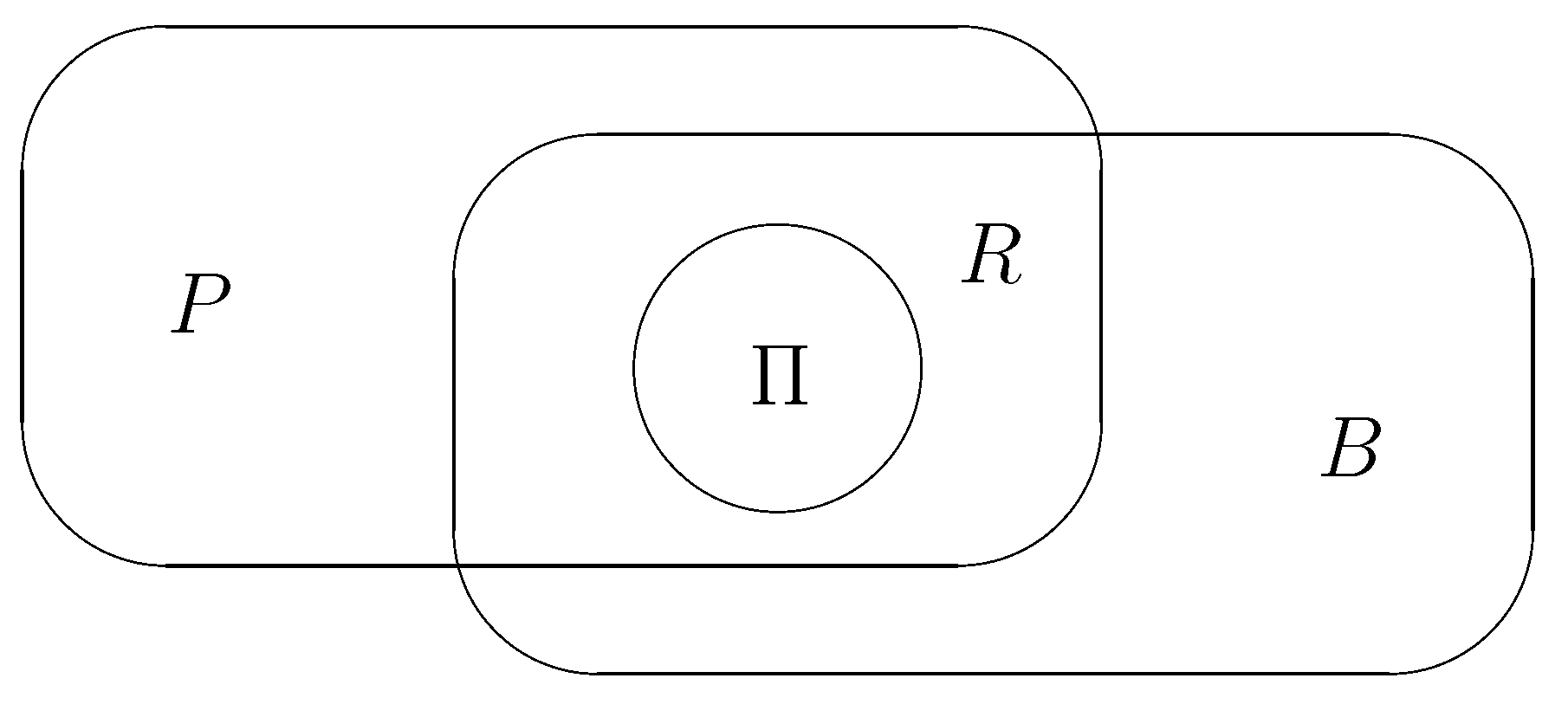
Let B, P, R and Π denote the sets of edge regular, vertex regular, regular and permutation-generated colourings respectively. The structural relations between colouring classes are summarised in the diagram displayed in Figure 8. In fact, we already saw examples of colourings in three of the four disjoint sets in the diagram. The colouring displayed in Figure 5(b) lies in P R , Figure 7(b) shows a colouring in Π and the colouring in Figure 6(b) lies in B R . (A graph colouring in R Π is given by ( V , E ) with V = [ 11 ] , V = { { 1 , 2 , 3 } , { 4 , 5 , 6 , 7 , 8 , 9 } , { 10 , 11 } } and E = { { 14 , 15 , 26 , 27 , 38 , 39 } , { ( 4 , 10 ) , ( 5 , 10 ) , ( 6 , 10 ) , ( 7 , 11 ) , ( 8 , 11 ) , ( 9 , 11 ) } } where ( i , j ) denotes an edge between vertices i and j.)
By Proposition 4.2, a graph colouring yields the same model restrictions representing an RCON model as it does representing an RCOR model if and only if it lies in B. Therefore, the model type only needs to be specified whenever a graph colouring lies in P B . Put formally:
Proposition 4.8.
For G = ( V , E ) C V , S + ( V , E ) = R + ( V , E ) for ( V , E ) B and S + ( V , E ) R + ( V , E ) for ( V , E ) P B . Thus if for X { B , P , R , Π } we let S X + denote the set of RCON models represented by graphs in X and similarly for R X + and RCOR models, then
S B + = R B + , S R + = R R + , S Π + = R Π + , S P + R P +
giving rise to five model classes lying strictly within S V + and R V + with
S Π + S R + S B + , S B + S P + = S B + R P + = S R + .
Let B V , P V , R V and Π V denote the sets of graph colourings inside B, P, R and Π with vertex set V. By Proposition 4.8, there are five corresponding model classes: S B V + , S P V + , R P V + , S R V + and S Π V + . For illustration we give the corresponding model class sizes for V = [ 4 ] together with | M [ 4 ] | in Table 1.
The relative sizes in Table 1 are representative of the general case: S B V + is the largest model class, followed by S P V + , R P V + and S R V + . | S P V + | = | R P V + | will generally be considerably smaller than S B V + as the defining conditions of P V are far more restrictive than those for B V . | S Π V + | is the smallest class of the four for all V, however may equal | S R V + | for some V, as for example for V = [ 4 ] .

5. Structures of Model Classes

Below we show that each model class defined above forms a complete non-distributive lattice, starting with S B V + and S Π V + as their structure turns out most tractable. For brevity, we only outline results for the remaining model classes.

5.1. Models Represented by Edge Regular Colourings

Proposition 5.1.
B V is stable under the meet operation ∧ in C V ; given in Equation (9).
Proof: 
Let G = ( V G , E G ) , H = ( V H , E H ) B V . G H = ( V G H , E G H ) is obtained from G and H by dropping of edge colour classes and merging of colour classes. The only operation potentially leading to G H lying outside of B V is merging of edge colour classes.
So let α β and γ δ be two edges in G H of equal colour. Then there exists a sequence α 0 β 0 , , α k β k in E G H such that α 0 β 0 = α β , α k β k = γ δ , and α i 1 β i 1 α i β i ( E G ) or α i 1 β i 1 α i β i ( E H ) for 1 i k . As both G and H have edge regular colourings, α i 1 β i 1 and α i β i connect the same vertex colour classes in the graph in which they are of equal colour, which we denote by { α i 1 , β i 1 } { α i , β i } ( V X ) with X { G , H } . This gives that { α , β } = { α 0 , β 0 } { α k , β k } = { γ , δ } ( V G V H ) . As V G V H = V G H , α β and γ δ connect the same vertex colour classes in G H . ☐
Graphs G 4 , G 5 and G 4 G 5 in Figure 4 illustrate the stability of B V under ∧. That B V is generally not stable under the join operation ∨ in Equation (9) is established by the example in Figure 9.
Proposition 5.2.
Let G = ( V , E ) C V and let E B be the partition of E which puts α β , γ δ E in the same set whenever they connect the same vertex color classes. Then G has a supremum in B V , given by
s B ( G ) = ( V , E E B )
Proof: 
The claim is trivially true for G B V . If G C V B V , an edge regular colouring cannot be achieved through splitting vertex colour classes or adding edge colour classes. The only effective manipulation is therefore the splitting of edge colour classes. The coarsest partition which is finer than E and gives an edge regular colouring is E E B , as it splits edge colour classes only if they connect different vertex colour classes. ☐
We deduce:
Theorem 5.3.
S B V + is a complete non-distributive lattice with respect to model inclusion. The meet operation is induced by the meet operation in C V ; given in Equation (9). The join of two models represented by graphs G , H B V is represented by the graph s B ( G H ) .
Proof: 
Proposition 5.1 implies that inf H exists for all finite H B V , which by Lemma 2.1 gives that B V is a complete lattice, with the same meet operation as C V ; . As the zero and unit in C V ; have edge regular colourings, they are also the zero and unit in B V .
By definition, for G , H B V , the join K of G and H in B V is the smallest graph with respect to partial ordering ⪯ which satisfies K G , K H and K B V . The supremum G H of G and H in C V ; is the smallest graph satisfying the first two relations so that K is in fact the smallest graph satisfying K ( G H ) and K B V . Thus G B H is given by the supremum of G H in B V , which by Proposition 5.2 equals s B ( G H ) .
Non-distributivity of B V is established by observing that Equation (4) is violated for a = G 6 , b = G 7 and c = G 8 displayed in Figure 10, as G 6 = G 6 ( G 7 G 8 ) ( G 6 G 7 ) ( G 6 G 8 ) = G 6 G 7 .
The results on the structure of B V naturally translate to the set of models S B V + , proving the claim. ☐

5.2. Models Represented by Permutation-Generated Colourings

Let Γ V denote the set of permutation groups acting on V. Then Γ V ; is a complete lattice [34] with meet and join operations given by Γ 1 Γ 2 = Γ 1 Γ 2 and Γ 1 Γ 2 = Γ 1 Γ 2 . We obtain:
Proposition 5.4.
Π V is stable under the meet operation ∧ in C V ; given in Equation (9). If G = ( V G , E G ) , H = ( V H , E H ) Π V are generated by Γ G , Γ H Γ V , then the colouring of G H is generated by Γ G Γ H .
Proof: 
Let G , H Π V and Γ G , Γ H Γ V be as in the claim. Then V G and E G are unions of orbits of Γ G in V and E G , and similarly for V H , E H and Γ H . By definition of the meet operation in C V ; , each vertex colour class in G H = ( V G H , E G H ) can be expressed as a union of vertex colour classes in V G , and as a union of vertex colour classes in V H , and similarly for the edges. Thus the colouring of G H is invariant under the action of both groups Γ G and Γ H , and therefore also under Γ G Γ H .
To show that the colouring of G H is generated by Γ G Γ H , we need to show that whenever two vertices or edges in G H are of the same colour, then there exists σ Γ G Γ H which maps one of them to the other. We present the argument for the edges only, as it is can be trivially transferred to the vertices. So let α β and γ δ be two edges in G H of equal colour. Then there exists a sequence α 0 β 0 , , α k β k in E G H such that α 0 β 0 = α β , α k β k = γ δ , and α i 1 β i 1 α i β i ( E G ) or α i 1 β i 1 α i β i ( E H ) for 1 i k . There must therefore exist σ i Γ G Γ H such that α i 1 β i 1 is mapped to α i β i by σ i for 1 i k , giving that the product σ k σ 1 Γ G Γ H maps α β to γ δ . ☐
Graphs G 4 , G 5 and G 4 G 5 in Figure 4 illustrate the above result, as each of the graphs lies in Π V , with generating groups Γ 4 = ( 13 ) ( 24 ) , Γ 5 = ( 13 ) and Γ 4 5 = Γ 4 Γ 5 = ( 13 ) , ( 24 ) respectively. Observing that the join G 4 G 5 , also displayed in Figure 4, does not lie in Π V establishes that Π V is generally not stable under the join operation in C V ; . However the following holds:
Proposition 5.5.
For G = ( V , E ) C V , let Aut ( V , E ) S ( V ) denote the largest group leaving ( V , E ) invariant and let ( V Aut , E Aut ) denote the graph colouring of G = ( V , E ) given by the orbits of Aut ( V , E ) in V and E respectively. Then G has a supremum in Π V given by
s Π ( G ) = ( V Aut , E Aut )
Proof: 
The claim is trivially true if G Π V . So suppose G C V Π V . G is modified to a larger graph by adding edge colour classes and splitting colour classes. As the former will not enforce a permutation-generated colouring, to prove the claim we need to that ( V Aut , E Aut ) is the coarsest refinement of ( V , E ) which lies in Π V . This is clearly the case as Aut ( V , E ) is the largest group which leaves V and E invariant. ☐
Theorem 5.6.
S Π V + is a complete non-distributive lattice with respect to model inclusion. The meet operation is induced by the meet operation in C V ; given in Equation (9). The join of two models represented by graphs G , H Π V is represented by the graph s Π ( G H ) .
Proof: 
The proof is analogous to the proof of Theorem 5.3. In brief, Proposition 5.4 and Lemma 2.1 give that Π V is a complete lattice with meet operation as claimed. As the zero and unit in C V ; have permutation-generated colourings, with Γ 0 = S ( V ) and Γ 1 = I d , they are the zero and unit in Π V .
By Proposition 5.5, the join of two graphs G , H Π V is given by s Π ( G H ) . The graphs displayed in Figure 10 establish non-distributivity of Π V as each of them has a permutation-generated colouring, with Γ 6 = ( 124 ) , Γ 7 = ( 234 ) , Γ 8 = ( 13 ) , ( 24 ) , Γ 7 8 = S ( [ 4 ] ) and Γ 6 7 = Γ 6 8 = ( 24 ) respectively. The above directly translate to S Π V + , proving the claim. ☐

5.3. Models Represented by Regular and Vertex Regular Colourings

The structures of R V and P V turn out to be closely related and it is for that reason that we treat them together. We abstain from giving explicit proofs of intermediate results for brevity, however give all facts the reader will require to construct them. We shall employ the notion of a factor graph:
Definition 5.7
([35]). Let f ( Y ) be a function in Y which factorises as f ( Y ) = Π i I f A i ( Y A i ) where A i V and f A i cannot be factorised further for i I . Then the factor graph of f is the graph G F = ( V F , E F ) with F = { f A i } i I being the set of factor vertices and E F = { α f A i α V , f A i F with α A i } .
For Y = ( Y α ) α V assumed to follow a N | V | ( μ , Σ ) distribution, the density f ( y ) factorises as
f ( y ) α V exp { k α α ( y α μ α ) 2 / 2 } · α , β V , α β exp { k α β ( y α μ α ) ( y β μ β ) }
giving that for the Gaussian distribution, either A i = { α } or A i = { α , β } for α , β V , with a factor being present if and only if the corresponding entry in Σ 1 is non-zero. Thus if the distribution of Y is assumed lie in the graphical Gaussian model represented by graph G = ( V , E ) , by Equation (3), each factor corresponds to a vertex in V or edge in E. The vertices in V can clearly be identified with their factors so that the factor graph of a graphical Gaussian model with graph G = ( V , E ) equals
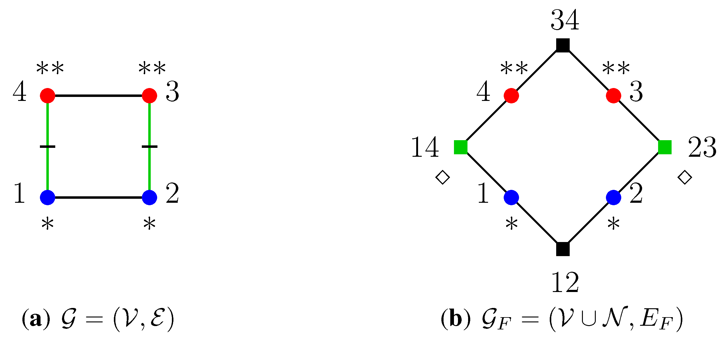
G F = ( V F , E F ) with F = { e e E } and E F = { α e α V , e E   is   incident   with α   in   G } .
This can be extended to the notion of a coloured factor graph, with an example given in Figure 11.
Definition 5.8.
For G = ( V , E ) C V representing a graphical Gaussian model with equality constraints, let N be a set of nodes with each node representing an edge in E and let N be the colouring of N in which nodes receive the same colour if and only if the corresponding edges are equally coloured in E . The coloured factor graph of the model is defined to be the vertex and node coloured graph G F = ( V N , E F ) with E F = { α n α V , n N and   n   represents   an   edge   incident   with   α } . The set of coloured factor graphs with vertex set V is denoted F V .
We give four intermediate results whose proofs we omit for brevity.
Lemma 5.9.
F V and C V are isomorphic. We denote the isomorphism by ϕ V : C V F V .
Lemma 5.10.
If G = ( V , E ) C V and ϕ V ( G ) = G F = ( V N , E F ) is the corresponding factor graph, then ( V , E ) R V if and only if ( V N ) is equitable with respect to G F = ( V N , E F ) .
Lemma 5.11
([36]). If P 1 and P 2 are two partitions of V both equitable with respect to the same graph G = ( V , E ) , then so is their join P 1 P 2 .
Lemma 5.12
([36]). For G = ( V , E ) and a partition P of V, (up to the order of cells) there exists a unique coarsest partition that is finer than P and equitable with respect to G, to be denoted by r G ( P ) .
Combined, Lemmas 5.9, 5.10 and 5.11 can be used to prove:
Proposition 5.13.
R V is stable under the meet operation ∧ in C V ; given in Equation (9).
Note that the graphs in Figure 4 illustrate the stability of R V under ∧ while showing that R V is generally not stable under ∨ in C V ; . Further, Lemma 5.12 implies:
Proposition 5.14.
Let G = ( V , E ) C V and let ϕ V ( G ) = G F = ( V N , E F ) be the corresponding coloured factor graph. Then G has a supremum in R V given by
s R ( G ) = ϕ V 1 ( ( r G F ( V N ) , E F ) )
We conclude:
Theorem 5.15.
S R V + is a complete non-distributive lattice with respect to model inclusion. The meet operation is induced by the meet operation in C V ; given in Equation (9). The join of two models represented by graphs G , H R V is represented by the graph s R ( G H ) .
Proof: 
The proof is analogous to the proofs of Theorems 5.3 and 5.6. ☐
Lemma 5.12 further implies:
Proposition 5.16.
P V is stable under the meet operation ∧ in C V ; given in Equation (9).
The graphs in Figure 4 also illustrate the stability of P V under ∧ while establishing that P V is generally not stable under ∨ in C V ; . Further:
Lemma 5.17.
If G = ( V , E ) C V and s R ( G ) = ( V R , E R ) , then for all G = ( V , E ) C V with V R V V , s R ( G ) = ( V R , E R ) .
Lemma 5.17 can be shown to imply:
Proposition 5.18.
For G = ( V , E ) C V let s R ( G ) = ( V R , E R ) . Then G has a supremum in P V given by
s P ( G ) = ( V R , E )
We conclude:
Theorem 5.19.
S P V + and R P V + are complete lattices with respect to model inclusion. Their meet operation is induced by the meet operation in C V ; given in Equation (9). The join of two models represented by G , H P V is represented by the graph s P ( G H ) .
Proof: 
In complete analogy to the proofs of Theorems 5.3 and 5.6. ☐

6. Model Selection

One way to develop model selection procedures for the model classes considered in this article is by adapting existing model search algorithms for unconstrained graphical Gaussian models. Having shown each of the model classes to be complete lattices, just as the set of standard graphical models, it is natural to consider methods which exploit this structural property. Prominent methods among them are stepwise procedures [24,25], the Edwards–Havránek model selection procedure [2], and, more recently, neighbourhood selection with the lasso [37], stability selection [38], and the SINful approach [39].
A crucial difference between the search spaces of unconstrained graphical Gaussian models and the models studied here is that while the former constitute a distributive lattice, the latter are all non-distributive. This directly disqualifies neighbourhood selection with the lasso, stability selection and the SINful approach, as they all require distributivity. Put explicitly, while the just mentioned methods are algorithms for determining for each edge whether it is to be present in graph of the accepted model(s) or not, for the model classes considered here not only the edge set needs to be determined, but also partitions of the vertices and present edges into sets corresponding to equal model parameters. This turns model selection into a principally different problem.
For the rest of the article we focus on the Edwards–Havránek model selection procedure and develop a corresponding algorithm for the lattice of models S B V + represented by edge regular colourings. We illustrate the algorithm with a brief summary of its, very encouraging, performance for the data set described in Example 3.1. We further give a summary of an Edwards–Havránek model search within the lattice of models S Π V + with permutation-generated colourings for the Fret’s heads data described in Example 4.7. All formal results are given without proof, however they can be obtained by considering the partial ordering of C V .

6.1. The Edwards–Havránek Model Selection Procedure

The Edwards–Havránek model selection procedure operates on model search spaces which are lattices and is closely related to the all possible models approach but considerably faster. It is based on the following two principles: (i) if a model is accepted then all models that include it are (weakly) accepted, and (ii) if a model is rejected then all of its submodels are considered to be (weakly) rejected.
The procedure starts by initially testing a set of models and assigns the accepted models to a set A and the rejected models to set R . By assumption, all models larger than A are (weakly) accepted and the ones smaller than R are (weakly) rejected, so that only min A , the smallest models in A , and max R , the largest models in R , are of interest. The procedure repeatedly updates min A and max R and terminates once the set to be updated remains unchanged, when it returns min A . The method to determine whether a model is to be rejected can be any suitable statistical test in accordance to the principle of coherence [40], stating that a test should not accept a model while rejecting a larger one.
Following [2], for a set of models S let D a ( S ) denote the set of models in the search lattice L say which are smallest with the property that they are not contained in any model in S,
D a ( S ) = min { d L d s   for   all   s S }
and let D r ( S ) be the set of largest models that do not contain any model in S,
D r ( S ) = max { d L s d   for   all   s S }
D a ( S ) is referred to as the acceptance dual of S, and D r ( S ) as the rejection dual of S. The procedure may then be summarised as:
  • Test an initial set of models and assign the accepted models to A and the rejected models to R .
  • Choose between 3 and 4.
  • Test the models in D r ( A ) R . If all are rejected, stop; otherwise, update A and R and go to 2.
  • Test the models in D a ( R ) A . If all are accepted, stop; otherwise, update A and R and go to 2.
Acceptance and rejection duals of sets of models can be computed in a recursive manner by using the following two relations. If S and T are two sets of models, then
D a ( S T ) = min { s t s D a ( S ) , t D a ( T ) } D r ( S T ) = max { s t s D r ( S ) , t D r ( T ) }
Thus describing the duals of a single model is enough.

6.2. Models with Edge Regular Colourings

Proposition 6.1.
Let S + ( V , E ) S B V + be a model represented by graph G = ( V , E ) with edge regular colouring and underlying uncoloured graph G = ( V , E ) . Then the acceptance dual D a ( S + ( V , E ) ) of S + ( V , E ) in S B V + contains all models represented by coloured graphs G a = ( V a , E a ) satisfying
(1i) 
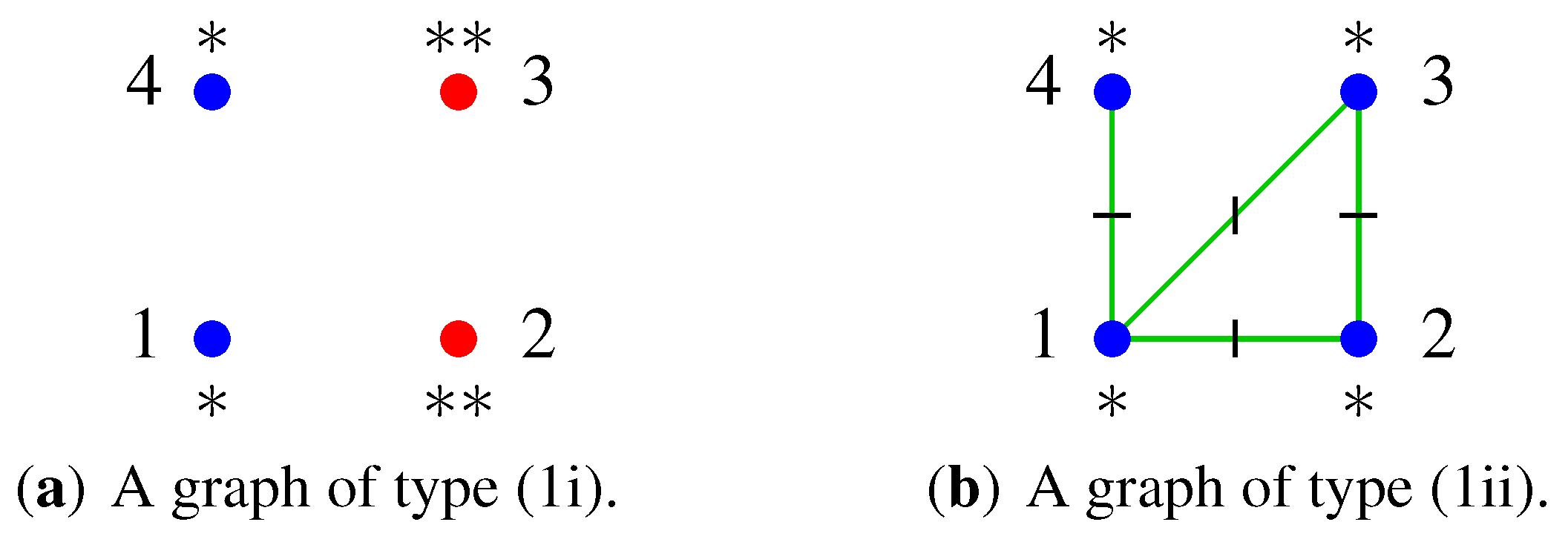
V a = { V 1 , V 2 } such that V a V and E a =
(1ii) 
V a = { V } and E a = { E a } with E a and E a E .
Put into words, models in the acceptance dual of S + ( V , E ) S B V + are either represented by the empty graph with two vertex colour classes which are not unions of colour classes in V , or they are represented by graphs in which all vertices are of the same colour, as are the edges, and the edge set is not a union of colour classes in E . For example, the coloured graphs in Figure 12 display models which lie in the acceptance dual of the model represented by the edge regular colouring in Figure 5(a).
By definition, acceptance duals are used to test whether there exist models immediately larger than max R which can be rejected. Effectively, graphs of type (1i) refine the colouring of the maximally rejected models, while graphs of type (1ii) add edge colour classes, which both give larger models.
Proposition 6.2.
Let S + ( V , E ) S B V + be a model represented by graph G = ( V , E ) with edge regular colouring and underlying uncoloured graph G = ( V , E ) , and for a discrete set A, let atom ( A ) denote the partition of A into atomic sets. Then the rejection dual D r ( S + ( V , E ) ) of S + ( V , E ) in S B V + contains all models represented by coloured graphs G r = ( V r , E r ) satisfying
(2i) 
V r = { { α , β } } atom ( V { α , β } ) such that V r V and E r = { α β α , β V } , or
(2ii) 
V r = atom ( V ) and E r = atom ( { α β α , β V } { e } ) with e E , or
(2iii) 
V r = { { α , β } , { γ , δ } } atom ( V { α , β , γ , δ } ) with α , β and γ , δ being of the same colour in V and E r = { { α γ , β δ } } atom ( { α β α , β V } { α γ , β δ } ) , where we may have α = β or γ = δ but not both, such that ( V , E ) ( V r , E r ) .
Graphs representing models in the rejection dual of a model represented by G = ( V , E ) almost represent the unrestricted saturated model except for a minor modification: In graphs of type (2i) two vertices which are not of the same colour in V form the only composite colour class in V r , while graphs of type (2ii) are missing an edge present in G = ( V , E ) . Graphs of type (2iii) have a pair of equally coloured edges which are not of the same colour in E , and give the end vertices of the edges an appropriate colouring for the graph colouring to be edge regular. Examples of coloured graphs representing models in the rejection dual of the model represented by the graph displayed in Figure 5(a) are given in Figure 13.
Rejection duals contain models which lie immediately below min A . Graphs of type (2i) merge vertex colour classes, graphs of type (2ii) cause edge colour classes to be dropped and graphs of type (2iii) merge edge colour classes, as well as vertex colour classes to ensure the resulting model to be edge regular. All operations give graphs which represent smaller models.
It can be shown that while | D a ( S + ( V , E ) ) | grows super-exponentially in the number of variables | V | (at rate O ( 2 | V | 2 / 2 ) ), the size of the rejection dual | D r ( S + ( V , E ) ) | grows polynomially in | V | (at rate O ( | V | 4 ) ), so that from a computational point of view working with rejection duals only is much more efficient. The following algorithm is therefore most efficient for models with edge regular colourings.
  • Test an initial set of models and assign each to R if it is rejected and to A otherwise.
  • Test the models in D r ( A ) R . If all are rejected, stop. Otherwise update A and R and repeat.
We executed the above algorithm for the Mathematics marks data set described in Example 3.1 with the saturated uncoloured model as our initial set of accepted models A and let R = initially. Models were tested for acceptance by performing a likelihood ratio test relative to the saturated unconstrained model at significance level 5 % using functionality implemented in the R package gRc [22]. The algorithm fitted 232 models, out of a total of 1.3 · 10 6 , in 8 stages before arriving at 4 minimally accepted models whose graphs are displayed in Figure 14 together with their BIC values. (The 232 models are distributed among the stages as follows. 1: 20 (6 accepted), 2: 21 (19 accepted), 3: 41 (40 accepted), 4: 56 (56 accepted), 5: 55 (55 accepted), 6: 29 (29 accepted), 7: 9 (9 accepted) and 8: 1 (1 accepted).)
The uncoloured graphs underlying the graphs in Figure 14 contain the graph in Figure 1(a) as a subgraph. G 1 , G 2 and G 3 only differ by one edge and G 4 has exactly the same edge set. Thus the conditional independence structures largely agree. The minimally accepted model with the lowest BIC value is represented by G 4 . It is different from but not dissimilar to the RCON model fitted in [1], whose graph is displayed in Figure 1(b), which has a slightly lower BIC value of 2587.404 but no specific properties and it is chosen in an ad hoc manner. Note that the model fitted in [1] is not edge regular so that it could not have been considered by the algorithm.
This example suggests that an Edwards–Havránek model selection procedure for models with edge regular colourings may be feasible in general.

6.3. Models Represented by Permutation-Generated Colourings

The class of permutation-generated colourings Π V is more complex in its structure than B V and therefore the duals D a ( S + ( V , E ) ) and D r ( S + ( V , E ) ) of a model S + ( V , E ) cannot be given in a purely combinatorial form in the graph colouring. A sound understanding of the relationship between a group Γ and its orbits in V and V × V is required in order to design a general algorithm, in principle, applicable to any variable set V. For illustrative purposes of the underlying principles we provide a brief summary of an Edwards–Havránek model search in S Π V + for Fret’s heads data described in Example 4.7.
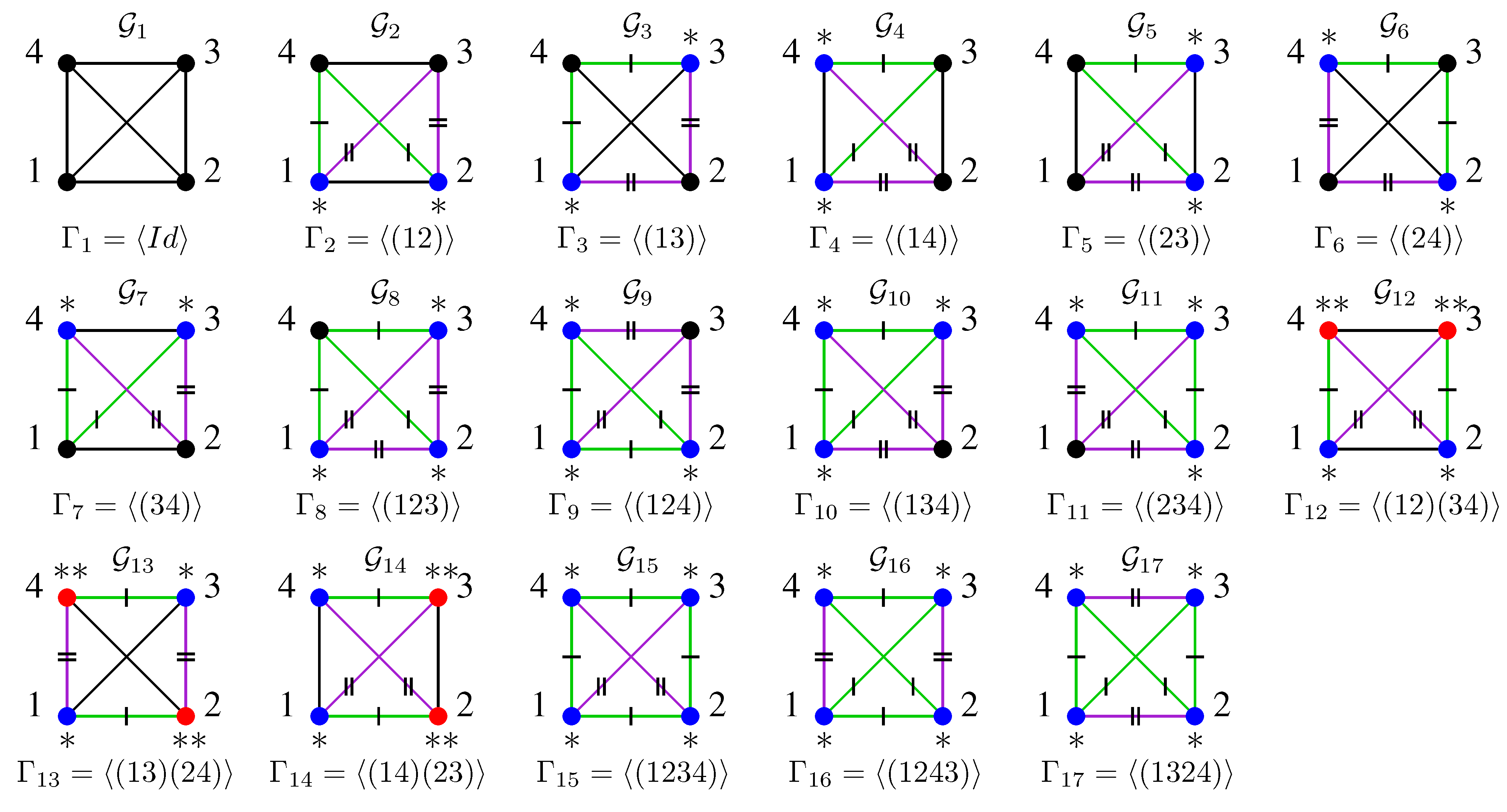
For V = { B 1 , B 2 , L 1 , L 2 } the symmetric group S ( V ) contains 4 ! = 24 permutations and has 30 subgroups, 17 of which are generated by a single permutation. Let K V denote the set of colourings of the complete graph these groups generate. The graph colourings in K V which are generated by a single permutation, i.e., by Γ = σ for σ S ( V ) , are displayed in Figure 15, where, for the sake of legibility we label the vertices by V = { 1 , 2 , 3 , 4 } . The remaining 13 subgroups generate only 5 distinct colourings in K [ 4 ] , all of which are shown in Figure 16 with one of their generating groups.
The search space Π [ 4 ] consists of all models which are represented by one of the 22 graphs in K [ 4 ] = { G 1 , , G 22 } displayed in Figure 15 and Figure 16, together with those represented by graphs which can be obtained from the above by dropping edge colour classes. Thus the size of the total search space is
| Π [ 4 ] | = N 1 + 6 N 2 + 4 N 8 + 3 N 12 + 3 ( N 15 1 ) + 3 ( N 18 4 ) + ( N 21 4 ) + N 22 = 2 6 + 6 · 2 4 + 4 · 2 2 + 3 · 2 4 + 3 ( 2 2 1 ) + 3 ( 2 3 4 ) + ( 2 3 4 ) + 2 = 251
where N i denotes the number of graphs one can obtain from graph G i . The subtracted correction terms prevent some graphs to be counted more than once.
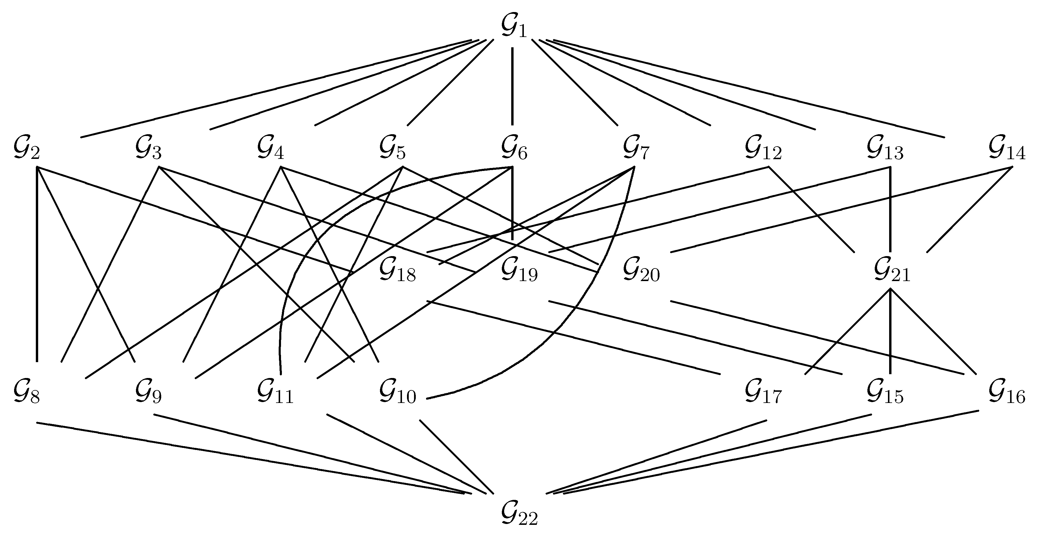
Figure 17 displays the Hasse diagram of K [ 4 ] . By construction, it contains only graphs which represent the saturated model. An Edwards–Havránek model selection procedure searches along the full Hasse diagram of all models in Π [ 4 ] , which contains all 251 models and has the diagram in Figure 17 as a subgraph. At each stage, the search moves along the edges in the diagram, passing each model at most once. Once a model has been rejected, all models below it are excluded from the future search; once a model has been accepted all models above it are excluded.
Exploiting the demonstrated lattice structure of Π [ 4 ] , we applied the algorithm to the Fret’s heads data described in Example 4.7 with A initially consisting of the saturated unrestricted model and R = . After testing 48 models in 4 stages the algorithm arrived at 9 minimally accepted models whose graphs and generating groups are given in Figure 18. (The models are distributed between the stages the following way. 1: 15 (9 accepted), 2: 16 (16 accepted), 3: 13 (13 accepted), 4: 4 (3 accepted).)
The minimally accepted model with the lowest BIC value is represented by graph H 9 , which is considerably less than the BIC value 471.2982 of the model fitted in [1] whose graph is displayed in Figure 7(b). Further, the model selected in [1] is a supermodel, in fact the supremum, of the models represented by H 7 and H 8 , with a further edge to complete the four cycle. Interestingly, H 2 and H 3 are two of the graphs found in Section 8.3 in [24], the other two being the underlying uncoloured graphs of H 7 and H 8 . Note that the BIC value of the complete symmetry model, whose graph is displayed on the right in Figure 7(b), lies between the smallest and the second smallest BIC values of the minimally accepted models, the corresponding graphs being H 9 and H 1 respectively. However it was (weakly) rejected by the procedure as it is a submodel of a model rejected in stage 1.

7. Discussion

As we argued, graphical Gaussian models with equality constraints are a promising model class as they combine parsimony in the number of parameters with the concise and efficient graphical models framework. We studied two model types introduced by [1]: RCON models which place equality restrictions on the model covariance matrix Σ 1 and RCOR models which restrict the diagonal of Σ 1 and the partial correlations, which can both be represented by vertex and edge coloured graphs.
We showed four model classes within the sets of RCON and RCOR models, each possessing desirable statistical properties and being more readily interpretable than RCON and RCOR models in general, to form complete non-distributive lattices. This qualifies each of them for an Edwards–Havránek model selection procedure. Two model classes, those represented by edge regular and permutation-generated colourings respectively, are most readily interpretable and possess the most tractable structure out of the four and are thus most suitable for a model search.
For the former model class we have developed an Edwards–Havránek model selection algorithm, and demonstrated an encouraging performance for the data set previously described in Example 3.1. We further illustrated the principal functionality of the Edwards–Havránek procedure on the lattice of models represented by permutation-generated colourings with the example of Fret’s heads data from Example 4.7. Here as well, the algorithm performed in a satisfactory fashion. In order to fully generalise it to work for any number of variables | V | , further investigation into the relationship between permutation groups acting on V and their orbits in V and V × V is necessary.
Some potential concerns need to be mentioned: firstly, while the algorithm’s performance in the above examples was encouraging, it has to be taken into account that the number of variables is rather small in both cases. Further, it is at this stage unknown how much this behaviour relied on strong/weak conditional independence and symmetry relations in the data sets considered. It may be that the number of models to be tested can still grow in an unmanageable fashion. Secondly, a general concern with the Edwards–Havránek model selection procedure is that its sampling properties are intractable. In particular the procedure does not control the overall error rate.
Especially in view of the above, it may be worthwhile to explore alternative model selection approaches. We argued that neighbourhood selection with the lasso [37], stability selection [38], and the SINful approach [39] were not directly applicable to the lattices of models studied in this article due to their non-distributivity. Modified variants may still be feasible, which could be investigated.
One further viable alternative may be a symmetry variant of the graphical lasso [41,42], which in its original form seeks to maximise the penalised log-likelihood
log det Σ 1 tr ( S Σ 1 ) ρ Σ 1 1
over non-negative definite matrices Σ 1 , with S denoting the empirical covariance matrix of the observations, tr ( · ) being the trace, · 1 the l 1 norm giving the sum of the absolute values of the elements in the argument matrix and ρ being the penalisation parameter. Testing for equality constraints on the entries of Σ 1 = ( k α β ) α , β V can be enforced by replacing Equation (12) by the following function
log det Σ 1 tr ( S Σ 1 ) ρ 1 Σ 1 1 ρ 2 α , β V | k α α k β β | ρ 3 α , β , γ , δ V , α β , γ δ | k α β k γ δ |
This lies in direct analogy to the development of the fused lasso [43] from the standard lasso for linear regression. However how to maximise the function for a given model class, for example over models with edge regular colourings to ensure scale invariance, seems non-trivial.

Acknowledgments

I would like to thank my PhD supervisor Steffen Lauritzen for many helpful discussions on the topic and Richard Samworth for inspiring conversations. I am very grateful to Michael Perlman and an anonymous referee for their constructive criticism of an earlier version of this article.

References

  1. Højsgaard, S.; Lauritzen, S.L. Graphical Gaussian models with edge and vertex symmetries. J. R. Stat. Soc. Ser. B 2008, 70, 1005–1027. [Google Scholar] [CrossRef]
  2. Edwards, D.; Havránek, T. A fast model selection procedure for large families of models. J. Am. Stat. Assoc. 1987, 82, 205–213. [Google Scholar] [CrossRef]
  3. Lauritzen, S.L. Graphical Models; Clarendon Press: Oxford, UK, 1996. [Google Scholar]
  4. Gottard, A.; Marchetti, G.M.; Agresti, A. Quasi-symmetric graphical log-linear models. Scand. J. Stat. 2011, 38, 447–465. [Google Scholar] [CrossRef]
  5. Ramírez-Aldana, R. Restricted or Coloured Graphical Log-Linear Models. PhD thesis, Graduate studies in Mathematics, National Autonomous University of Mexico, Mexico City, Mexico, 2010. [Google Scholar]
  6. Uhler, C. Geometry of Maximum Likelihood Estimation in Gaussian Graphical Models. 2010. Available online: http://arxiv.org/abs/1012.2643 (accessed on 2 September 2011).
  7. Wilks, S.S. Sample criteria for testing equality of means, equality of variances, and equality of covariances in a normal multivariate distribution. Ann. Math. Stat. 1946, 17, 257–281. [Google Scholar] [CrossRef]
  8. Votaw, D.F. Testing compound symmetry in a normal multivariate distribution. Ann. Math. Stat. 1948, 19, 447–473. [Google Scholar] [CrossRef]
  9. Olkin, I.; Press, S.J. Testing and estimation for a circular stationary model. Ann. Math. Stat. 1969, 40, 1358–1373. [Google Scholar] [CrossRef]
  10. Olkin, I. Testing and Estimation for Structures Which Are Circularly Symmetric in Blocks; Technical Report; Educational Testing Service: Princeton, NJ, USA, 1972. [Google Scholar]
  11. Andersson, S.A. Invariant normal models. Ann. Math. Stat. 1975, 3, 132–154. [Google Scholar] [CrossRef]
  12. Jensen, S.T. Covariance hypotheses which are linear in both the covariance and the inverse covariance. Ann. Stat. 1988, 16, 302–322. [Google Scholar] [CrossRef]
  13. Hylleberg, B.; Jensen, M.; Ørnbøl, E. Graphical Symmetry Models. Master’s thesis, Aalborg University, Aalborg, Denmark, 1993. [Google Scholar]
  14. Andersen, H.H.; Højbjerre, M.; Sørensen, D.; Eriksen, P.S. Linear and Graphical Models for the Multivariate Complex Normal Distribution; Springer Verlag: New York, NY, USA, 1995. [Google Scholar]
  15. Madsen, J. Invariant normal models with recursive graphical Markov structure. Ann. Stat. 2000, 28, 1150–1178. [Google Scholar] [CrossRef]
  16. Gehrmann, H.; Lauritzen, S. Estimation of Means on Graphical Gaussian Models with Symmetries. 2011. Available online: http://arxiv.org/abs/1101.3709 (accessed on 2 September 2011).
  17. Frets, G.P. Heredity of head form in man. Genetica 1921, 41, 193–400. [Google Scholar] [CrossRef]
  18. Mardia, K.V.; Kent, J.T.; Bibby, J.M. Multivariate Analysis; Academic Press: New York, NY, USA, 1979. [Google Scholar]
  19. Bollobás, B. Modern Graph Theory; Springer Verlag: New York, NY, USA, 1998. [Google Scholar]
  20. Grätzer, G. General Lattice Theory; Birkhäuser Verlag: Basel, Switzerland, 1998. [Google Scholar]
  21. Brown, L.D.; Author, T. Fundamentals of Statistical Exponential Families with Applications in Statistical Decision Theory; Gupta, S.S., Ed.; Institute of Mathematical Statistics: Hayward, CA, USA, 1986. [Google Scholar]
  22. Højsgaard, S.; Lauritzen, S.L. Inference in graphical Gaussian models with edge and vertex symmetries with the gRc package for R. J. Stat. Softw. 2007, 23. [Google Scholar] [CrossRef]
  23. Anderson, T.W. Estimation of Covariance Matrices which are Linear Combinations or Whose Inverses are Linear Combinations of Given Matrices. In Essays in Probability and Statistics; Bose, R.C., Chakravati, I.M., Mahalanobis, P.C., Rao, C.R., Smith, K.J.C., Eds.; University of North Carolina Press: Chapel Hill, NC, USA, 1970; pp. 1–24. [Google Scholar]
  24. Whittaker, J. Graphical Models in Applied Multivariate Statistics; Wiley: Chichester, UK, 1990. [Google Scholar]
  25. Edwards, D. Introduction to Graphical Modelling; Springer Verlag: New York, NY, USA, 2000. [Google Scholar]
  26. Cox, D.R.; Wermuth, N. Linear dependencies represented by chain graphs (with discussion). Stat. Sci. 1993, 8, 204–218, 247–277. [Google Scholar] [CrossRef]
  27. Bell, E.T. Exponential numbers. Am. Math. Mon. 1934, 1, 411–419. [Google Scholar] [CrossRef]
  28. Pitman, J. Probabilistic aspects of set partitions. Am. Math. Mon. 1997, 104, 201–209. [Google Scholar] [CrossRef]
  29. Dobiński, G. Summierung der Reihe ∑nm/n! für m = 1,2,3,4,5,…. Grunert Arch. (Arch. Math. Phys.) 1877, 61, 333–336. [Google Scholar]
  30. Complet, P. Advanced Combinatorics; D. Reidel Publishing Company: Boston, MA, USA, 1974. [Google Scholar]
  31. Sachs, H. Über teiler, faktoren und charakteristische polynome von graphen. Wiss. Z. Tech. Hochsch. Ilmenau 1966, 12, 7–12. [Google Scholar]
  32. Siemons, J. Automorphism groups of graphs. Arch. Math. 1983, 41, 379–384. [Google Scholar] [CrossRef]
  33. Buhl, S. On the existence of maximum likelihood estimators for graphical Gaussian models. Scand. J. Stat. 1993, 20, 263–270. [Google Scholar]
  34. Schmidt, R. Subgroup Lattices of Groups; de Gruyter: Berlin, Germany, 1994. [Google Scholar]
  35. Frey, B.; Kschischang, F.; Loelinger, H.; Wiberg, N. Factor Graphs and Algorithms. In Proceedings of the 35th Allerton Conference on Communication, Control and Computing, Allerton House, Monticello, IL, USA, 29 September–1 October 1997. [Google Scholar]
  36. McKay, B. Backtrack Programming and the Graph Isomorphism Problem. Master’s thesis, University of Melbourne, Parkville, VIC, Australia, 1976. [Google Scholar]
  37. Meinshausen, N.; Bühlmann, P. High dimensional graphs and variable selection with the lasso. Ann. Stat. 2006, 34, 1436–1462. [Google Scholar] [CrossRef]
  38. Meinshausen, N.; Bühlmann, P. Stability selection. J. R. Stat. Soc. Ser. B 2010, 72, 417–473. [Google Scholar] [CrossRef]
  39. Drton, M.; Perlman, D. A SINful Approach to Gaussian graphical model selection. J. Stat. Plan. Inference 2008, 7138, 1179–1200. [Google Scholar] [CrossRef]
  40. Gabriel, K.R. Simultaneous test procedures—some theory of multiple comparisons. Ann. Math. Stat. 1969, 40, 224–250. [Google Scholar] [CrossRef]
  41. Friedman, F.; Hastie, T.; Tibshirani, R. Sparse inverse covariance estimation with the graphical lasso. Biostatistics 2008, 9, 432–441. [Google Scholar] [CrossRef] [PubMed]
  42. Ravikumar, P.; Wainwright, M.J.; Raskutti, G.; Yu, B. High-Dimensional Covariance Estimation by Minimizing l1-Penalized Log-Determinant Divergence. In Proceedings of the 22nd Annual Conference on Neural Information Processing Systems (NIPS), Vancouver, BC, Canada, 8–10 December 2008. [Google Scholar]
  43. Tibshirani, R.; Saunders, M.; Rosset, S.; Zhu, J.; Knight, K. Sparsity and smoothness via the fused lasso. J. R. Stat. Soc. Ser. B 2005, 67, 91–108. [Google Scholar] [CrossRef]
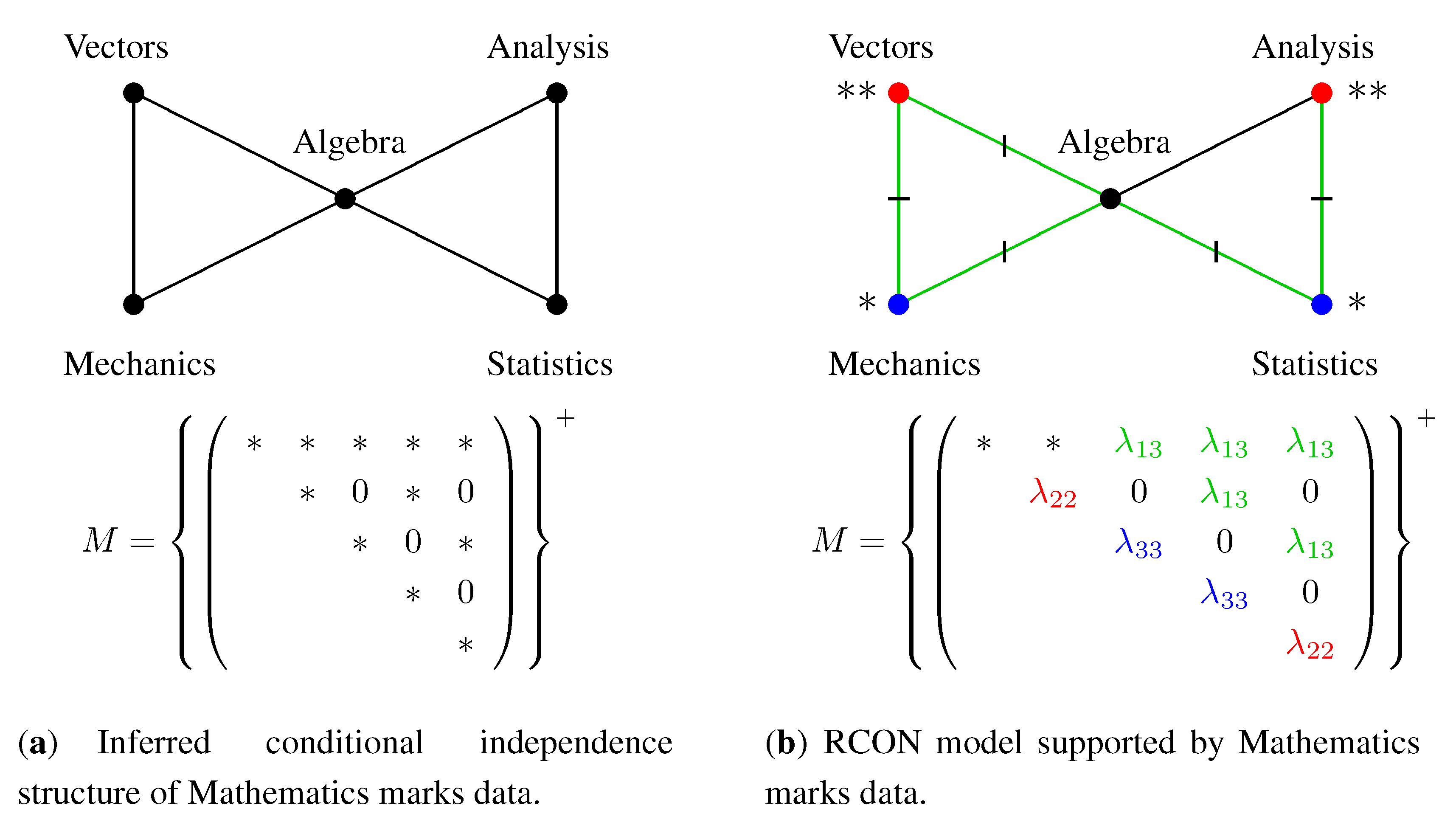
Figure 1. Mathematics marks example.
Symmetry 03 00653 g001
Figure 2. Personality characteristics example.
Symmetry 03 00653 g002
Figure 3. Partial ordering in C [ 4 ] .
Symmetry 03 00653 g003
Figure 4. Meet and join operations in C [ 4 ] .
Symmetry 03 00653 g004
Figure 5. An edge regular colouring and one which is not edge regular.
Symmetry 03 00653 g005
Figure 6. A vertex regular colouring and one which is not vertex regular.
Symmetry 03 00653 g006
Figure 7. Frets’ heads example.
Symmetry 03 00653 g007
Figure 8. Structural relations between colouring classes.
Symmetry 03 00653 g008
Figure 9. B [ 4 ] is not stable under ∨.
Symmetry 03 00653 g009
Figure 10. Non-distributivity of B V .
Symmetry 03 00653 g010
Figure 11. A coloured graph and the corresponding coloured factor graph.
Symmetry 03 00653 g011
Figure 12. Acceptance dual corresponding to the graph in Figure 5(a).
Symmetry 03 00653 g012
Figure 13. Rejection dual corresponding to the graph in Figure 5(a).
Symmetry 03 00653 g013
Figure 14. Graphs of minimally accepted models in S B [ 5 ] + .
Symmetry 03 00653 g014
Figure 15. Colourings in K [ 4 ] which are generated by Γ = σ for some σ S ( V ) .
Symmetry 03 00653 g015
Figure 16. Remaining colourings in K [ 4 ] .
Symmetry 03 00653 g016
Figure 17. Hasse diagram of K [ 4 ] .
Symmetry 03 00653 g017
Figure 18. Graphs of minimally accepted models in Π [ 4 ] for Frets’ heads data.
Symmetry 03 00653 g018
Table 1. Model set sizes for V = [ 4 ] .
Model class S [ 4 ] + , R [ 4 ] + S B [ 4 ] + S P [ 4 ] + , R P [ 4 ] + S R [ 4 ] + S Π [ 4 ] + M [ 4 ]
Size13,1553065138025125164