1. Introduction
Do there exist spherically symmetric distributions on the closed unit ball in that have uniform one-dimensional marginal distributions on ? A distribution on with this property may be said to “square the circle” when and to “cube the sphere” when .
The cumulative distribution function (cdf) of a multivariate distribution on the unit cube
whose marginal distributions are uniform
is commonly called a
copula; see Nelsen [
1] for an accessible introduction to this topic. However, although it is customary to confine attention to distributions on the
unit cube, our interest is in
spherically symmetric (= orthogonally invariant) distributions on with uniform marginal distributions. Therefore we take “copula” to mean a multivariate cdf on the
centered cube
with uniform
marginals.
For (resp., ), such a copula, if it exists, will be called a circular copula (resp., spherical copula) if it is the cdf of a circularly symmetric (resp., spherically symmetric) distribution on the unit disk (resp., unit ball ).
It will be noted in
Section 2 and
Section 3 that circular and spherical copulas are unique if they exist, but exist only for dimensions
and
. The proof of non-existence for
is remarkably simple. Explicit expressions for these copulas are given in
Section 3 and
Section 4 respectively.
In
Section 5, a new one-parameter family of bivariate copulas called
elliptical copulas is obtained from the unique circular copula in
by oblique coordinate transformations. Finally, in
Section 6, copulas obtained by a non-linear transformation of a uniform distribution on the unit ball in
are described, and determined explicitly for
.
3. The Bivariate Case: The Unique Circular Copula
The following three questions constitute an engaging classroom exercise.
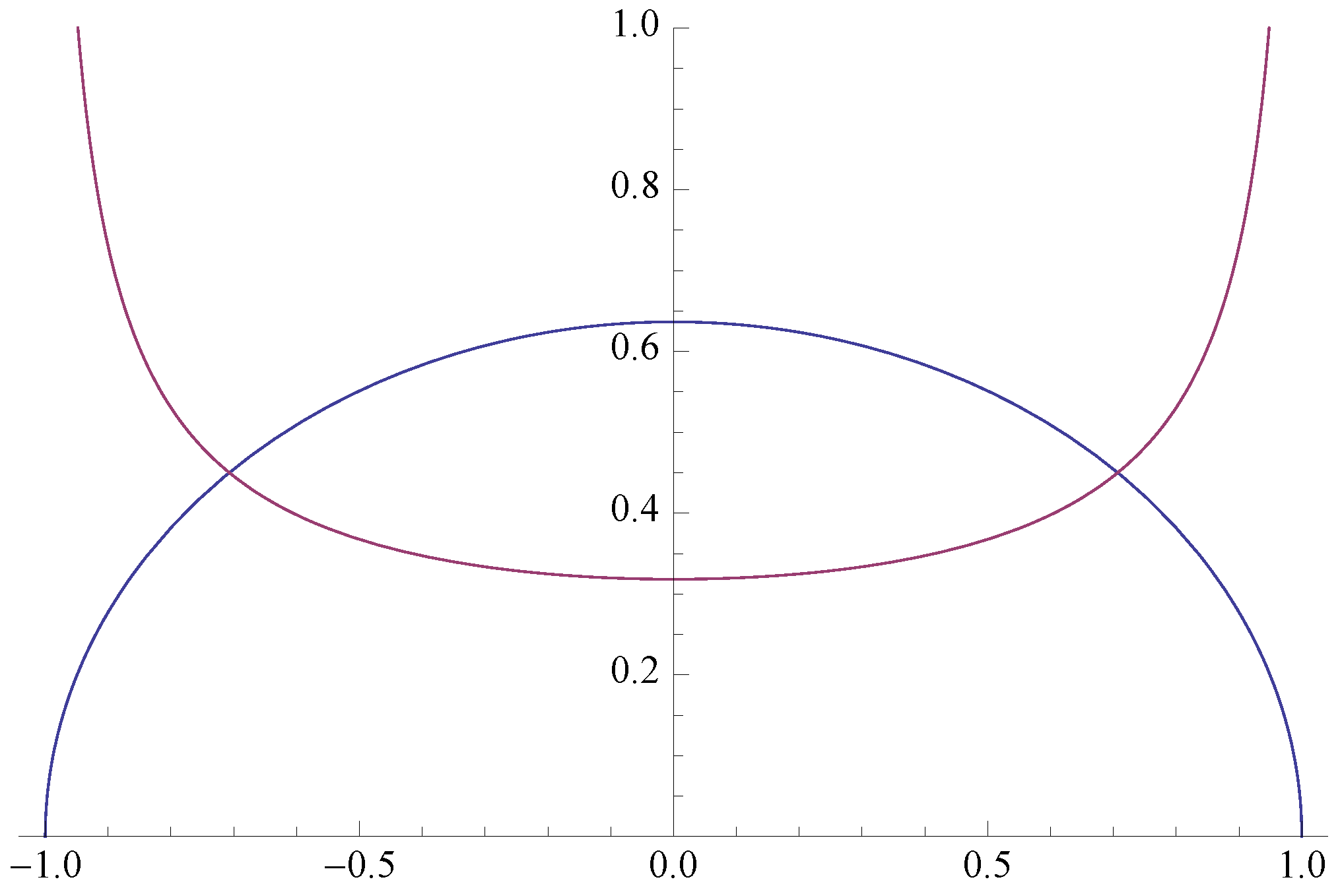
Question 1. Let be a random vector uniformly distributed on the unit disk (= ball) in . Find the marginal probability distributions of X and Y.
Answer: One can easily show that
X has the “semi-circular” probability density function (pdf) given by
(See
Figure 1.) By symmetry,
Y has the same pdf as
X.
Question 2. Let be a random vector uniformly distributed on the unit circle in . Find the marginal probability distributions of X and Y.
Answer: We can represent
as
where
. It follows readily that
X has pdf
(See
Figure 1.) By symmetry,
Y has the same pdf as
X.
In both cases, the joint distribution of
is circularly symmetric, that is, invariant under all orthogonal transformations of
. A comparison of the shapes of the pdfs in
Figure 1 suggest a third question:
Question 3. Does a circularly symmetric bivariate distribution with uniform
marginals exist on
? If so, it determines a circular copula on
, which is unique by Proposition 2.1. This also follows from uniqueness results for the Abel transform; see, e.g., Bracewell [
6].
Answer: Optimistically, let’s seek an absolutely continuous solution. That is, we seek a bivariate pdf on
of the form
such that the marginal pdf
is constant in
x. Here
g is a nonnegative function on
that must satisfy
in order that
(transform to polar coordinates:
).
To determine a suitable
g, first set
, then let
to obtain
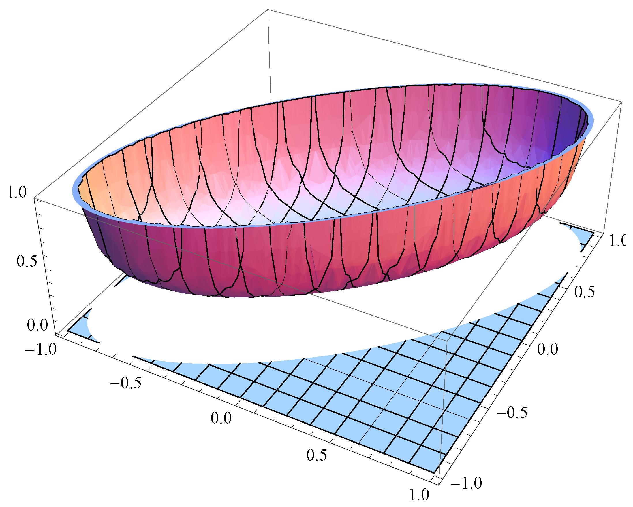
If we take
then clearly
does not depend on
x, and choosing
satisfies (
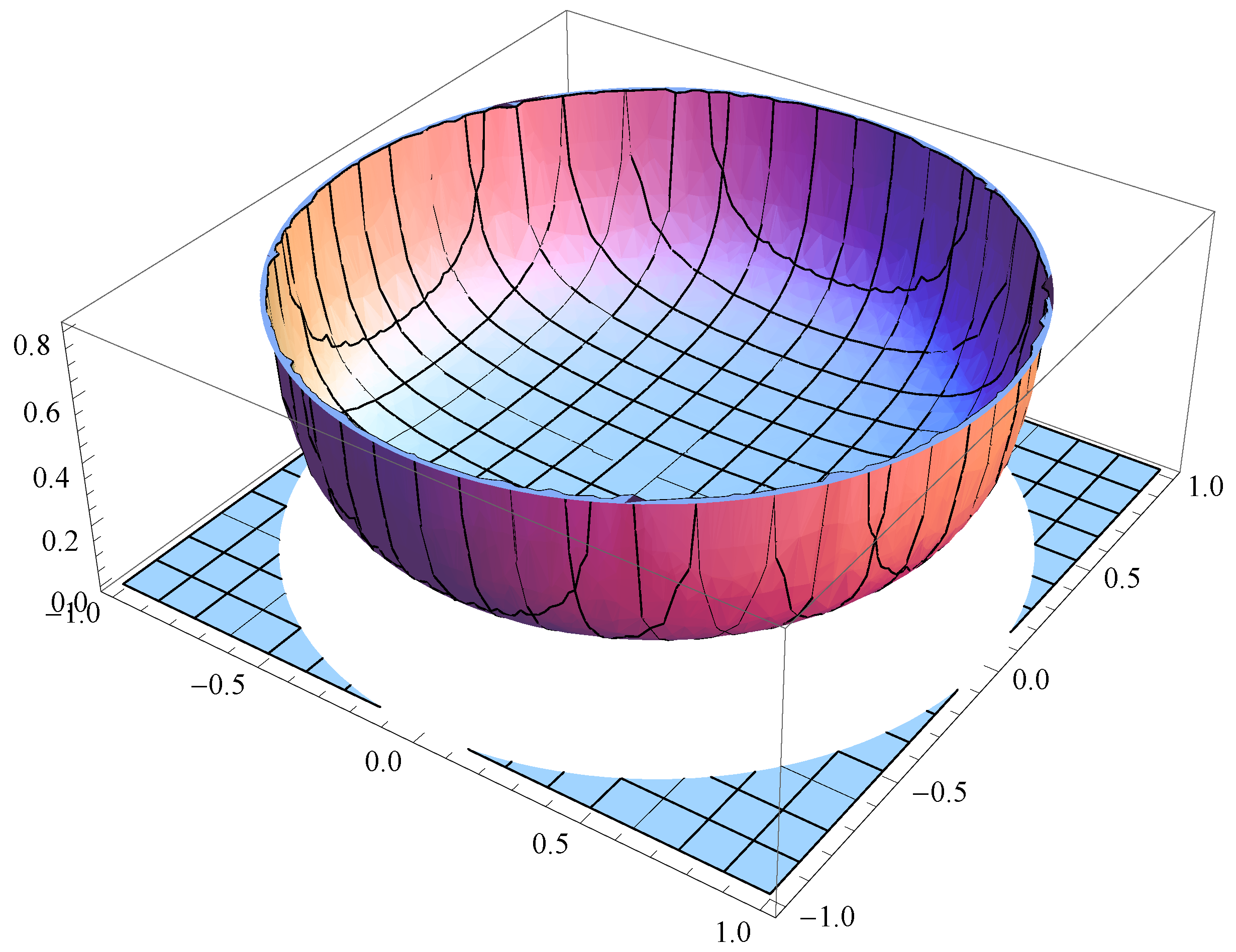
5). Thus the bivariate pdf (see
Figure 2)
determines a circularly symmetric bivariate distribution on
and yields the desired circular copula.
Question 4. Having determined the unique circularly symmetric distribution (
6) on
with uniform marginals, what is the corresponding cdf
, that is, what is the corresponding circular copula?
Answer (see Theorem 3.1): The circular symmetry of
implies that its distribution is invariant under sign changes,
i.e.,
. By the following lemma, the cdf
on
can be expressed in terms of
, its truncation to the first quadrant:
for
, and also in terms of the complementary cdf
for
. Because
and has uniform
marginals,
Lemma 3.1. Let be a bivariate random vector on with uniform marginal distributions and sign-change invariance, i.e., . Then for ,where if and . Proof. To obtain (
9), consider four cases:
Case 1: . Because
is sign-change invariant and has uniform
marginals,
Case 2: . Similarly,
Case 3: . Similarly,
Case 4: . Similarly,
Finally, (10) follows from (
9) by (
8). □
Thus, to determine the circular copula
for the pdf (
6), it suffices to determine the complementary cdf
for
and apply (10). Because
when
, we need only consider the case where
.
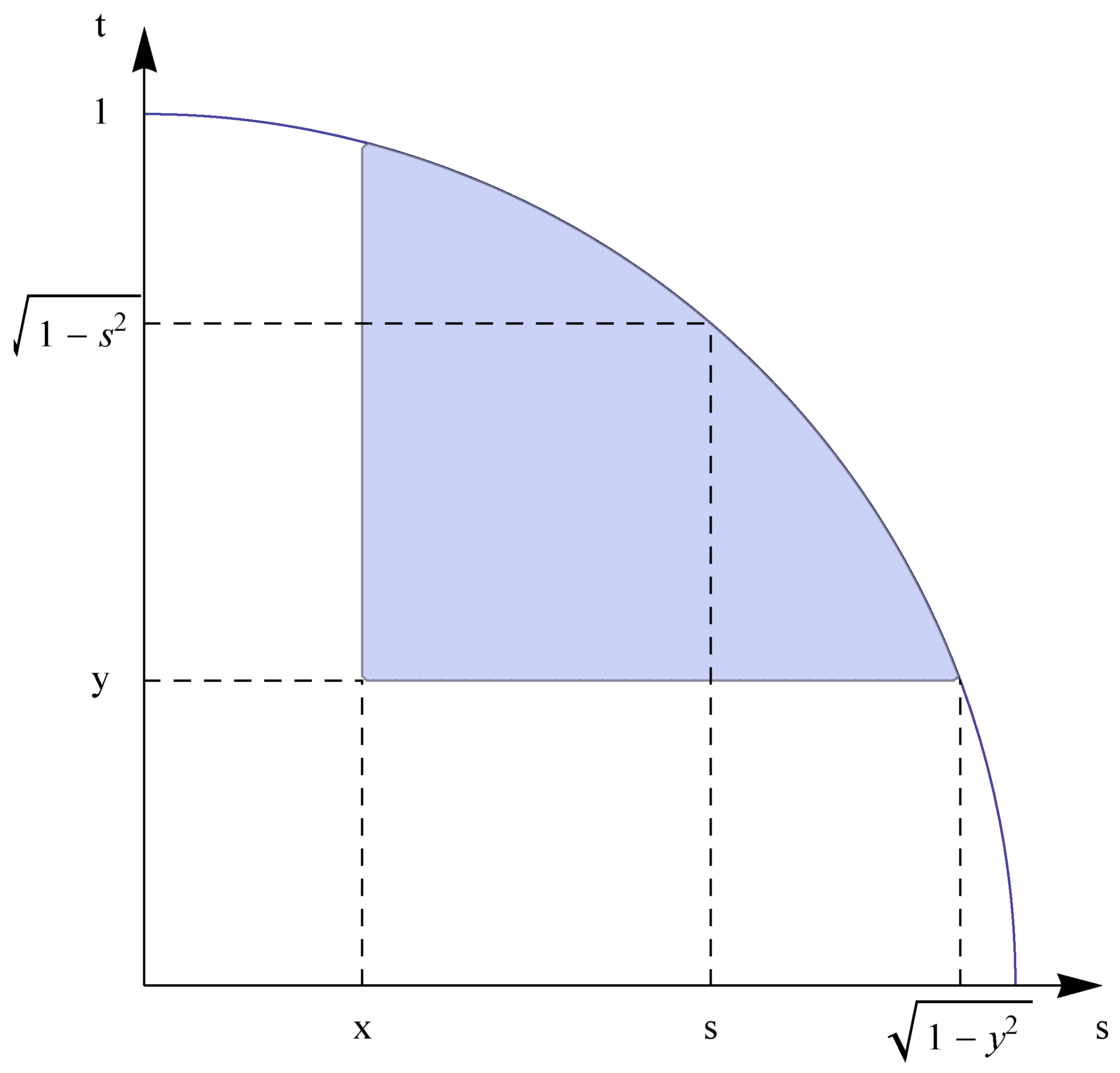
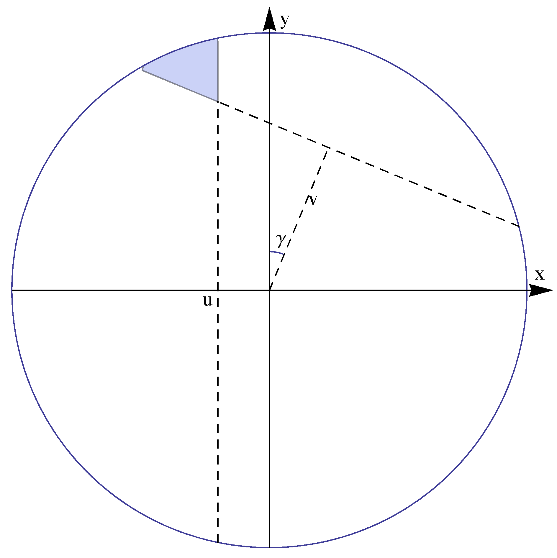
First approach: When
and
,
can be expressed as follows. By using
Figure 3 we find that
However, we were unable to evaluate this integral directly.
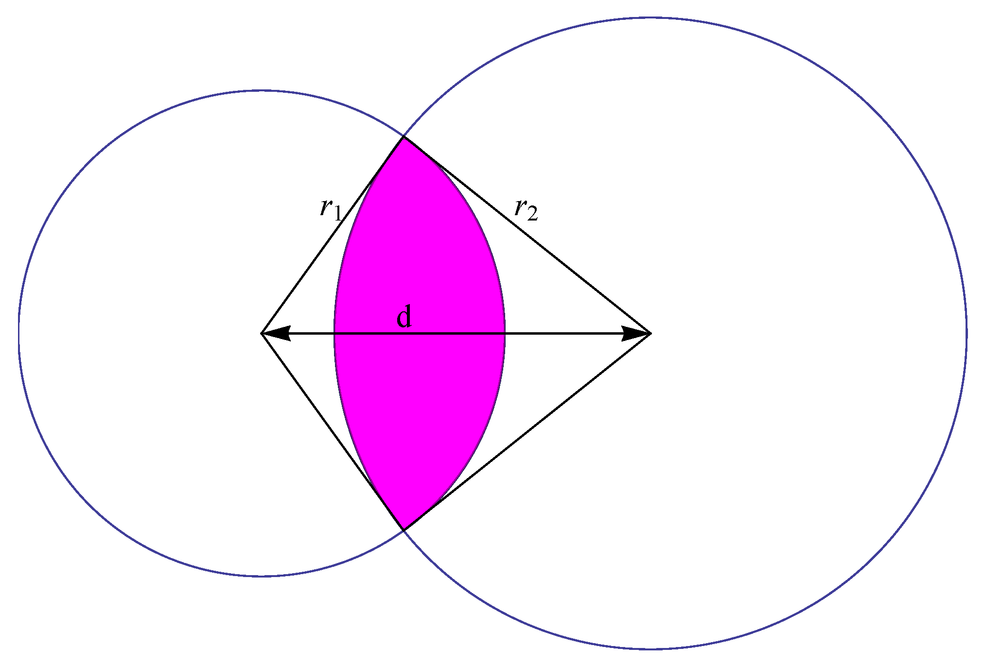
Second approach: Fortunately, we have found a solution in the molecular biology and optics literatures, where the problem of finding the area of the intersection of two spherical caps on the unit sphere
has been addressed. The following general result is due to Tovchigrechko and Vakser [
7] and also appears in Oat and Sander [
8].
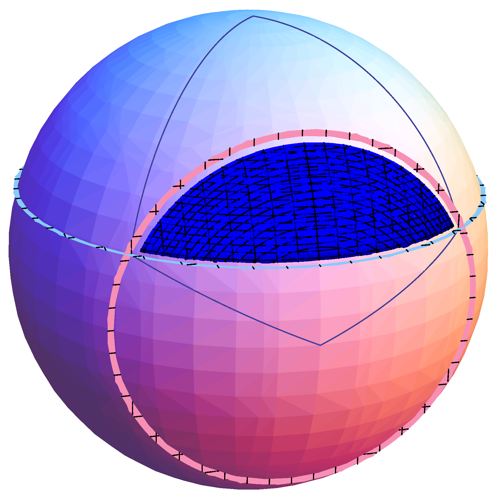
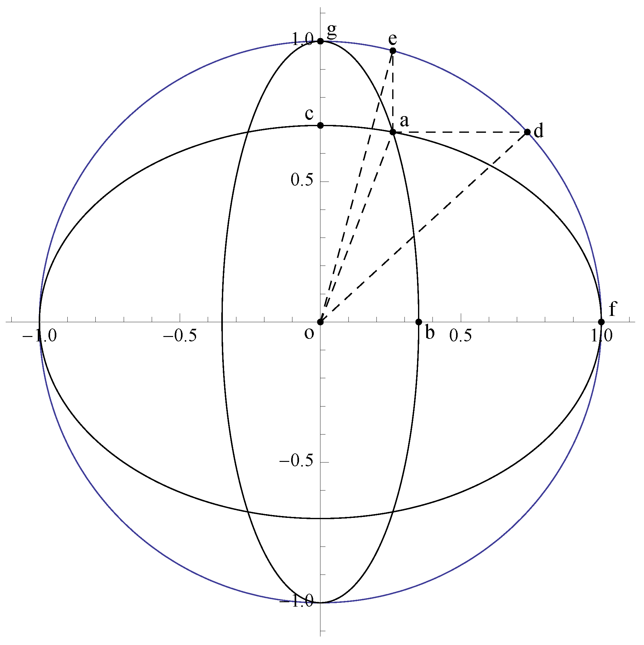
Lemma 3.2. Let and be spherical caps on . Let and denote their angular radii and let d denote the angular distance between their centers (). Assume that and , so that the intersection and consists of a single “diangle”; (see Figure 4 and Figure 5.) Then Area is given by This result can be applied to obtain our desired circular copula as follows.
If
is uniformly distributed on
, then the event
corresponds to the intersection of the two spherical caps
and
, so
is given by the area
of this intersection divided by the total area of
,
i.e., by
. (See
Figure 4 and
Figure 5.) Also, the joint distribution of
is circularly symmetric on the unit disk
and has uniform marginals, so must be the unique such bivariate distribution, namely the distribution with pdf (
6).
Thus, for
and
, our desired complementary cdf is given by
where for
and
,
Theorem 3.1. The unique circular copula on is given bywhere is defined by (16) for and byfor . Note that Equations (16) and (18) agree when and both are sign-change equivariant on : for all and all , Proof. From Equations (10) and (15), when
we have
by (
19). When
,
so (
17) again holds by (10) and (
18). □
See
Figure 6 for a plot of the resulting copula (on
).
4. The Trivariate Case: the Unique Spherical Copula
Question 5. Having determined the unique spherically symmetric distribution on with uniform marginals, namely, the uniform distribution on the unit sphere , what is the corresponding cdf on , i.e., the unique spherical copula?
Answer: As in
Section 3, let
be uniformly distributed on
, so that
. Again we first determine the complementary cdf
for
and
, the intersection of the first octant of
with the interior of
. Here the event
corresponds to the intersection of the three spherical caps
,
, and
on
, so
is the area
of this intersection divided by the total area
of
.
Recall that two approaches were proposed in
Section 3 to obtain the area
of the intersection of
two circular caps
and
. The first approach led to the integral (
11) that we were unable to evaluate explicitly, so we adopted a second approach based on the geometric Lemma 3.2 of Tovchigrechko and Vakser [
7]. Andrey Tovchigrechko has kindly suggested a method for extending Lemma 3.2 to the case of three spherical caps in general position, which if carried out would yield an explicit expression for
. However, we have found that because the axes of our three caps are mutually orthogonal, the two approaches just mentioned for the bivariate case can be combined to obtain
directly for the trivariate case, as now described.
We begin by extending (
11) to obtain an integral expression for
when
and
. We require the fact that
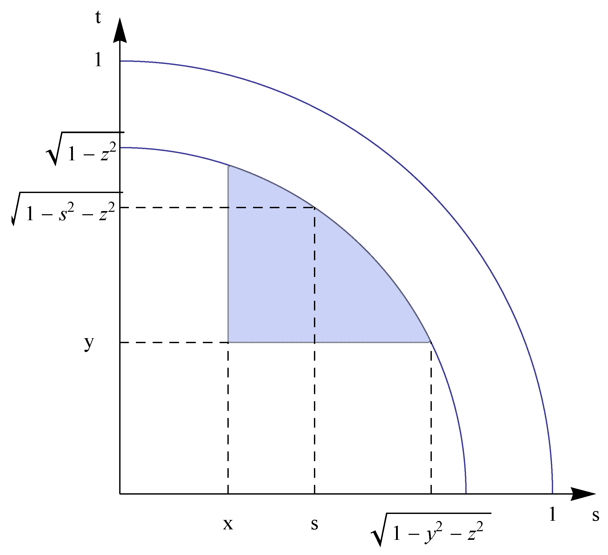
Lemma 4.1. If and , then Because is exchangeable, (23) remains valid under any permutation of on the right-hand side. Proof. Since
and
, it follows from (
6) by using
Figure 7 that
Now apply (
22) to obtain (
23). □
As noted above, the integral in (
23) appears difficult to evaluate explicitly but the following indirect argument succeeds. Recall from (
11) and (15) that when
and
,
where
is given by (
16). Because
when
and
, it follows that
Therefore from (
23) and (
24), if
and
then
By (
22), however,
so if we define
by
for
and
, then
where
is given by (
16). Now (
22) gives
so the above simplifies to
where
a symmetric function of
. By (
22), however,
and
so
, hence
identically in
. Therefore we conclude that
for
and
.
We now apply (
28) to obtain the cdf
for all
. For this, extend the definition of
in (
27) to all
by means of (
16) and (
18).
Theorem 4.1. The unique spherical copula on is given as follows:
for , 5. A One-Parameter Family of Elliptical Copulas
Let
in (
6), the unique circularly symmetric distribution on the unit disk
with uniform
marginals. For any angle
, consider the transformed variables
By the circular symmetry of
,
, so the random vector
again generates a copula on the centered square
. Denote the pdf and cdf of
by
and
respectively. Then
is a one-parameter family of
elliptical copulas, so-called because the support of
is the ellipse
(Note that
.) From (
29), the correlation coefficient of
U and
is given simply by
so
indicates the degree of linear dependence between
U and
.
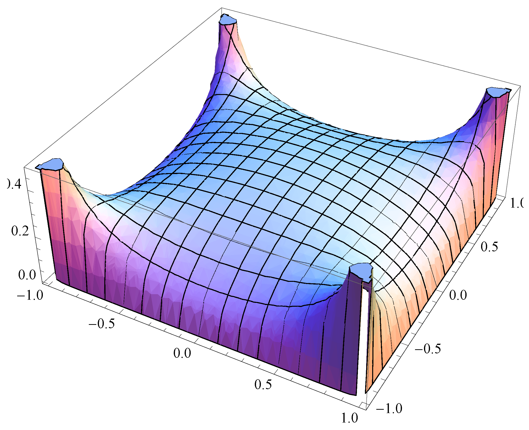
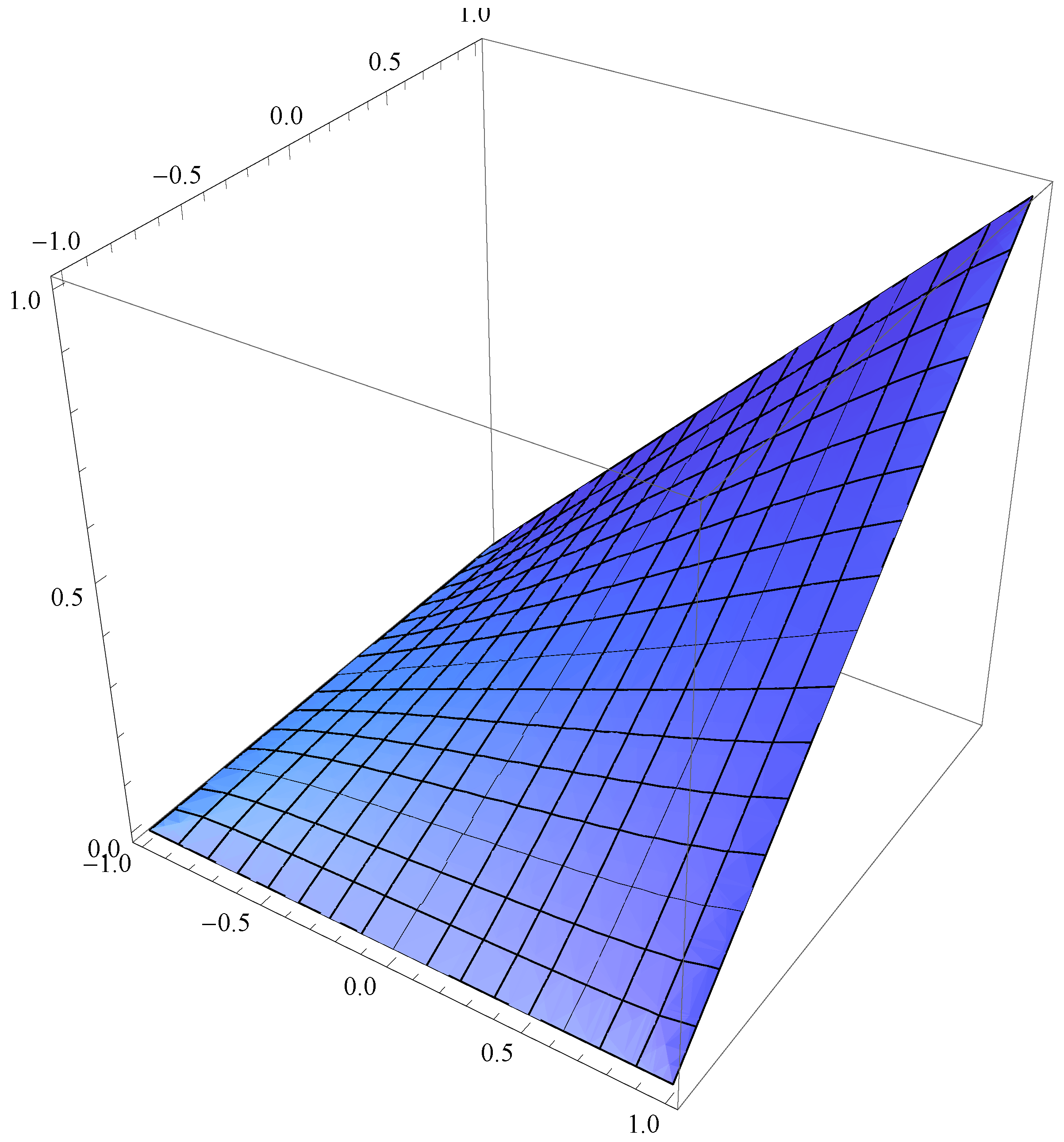
Proposition 5.1. The pdf of is given by Proof. The pdf can be obtained by a standard Jacobian computation. From (
29),
so
Thus the Jacobian of the transformation is
, so from (
6) we obtain
□
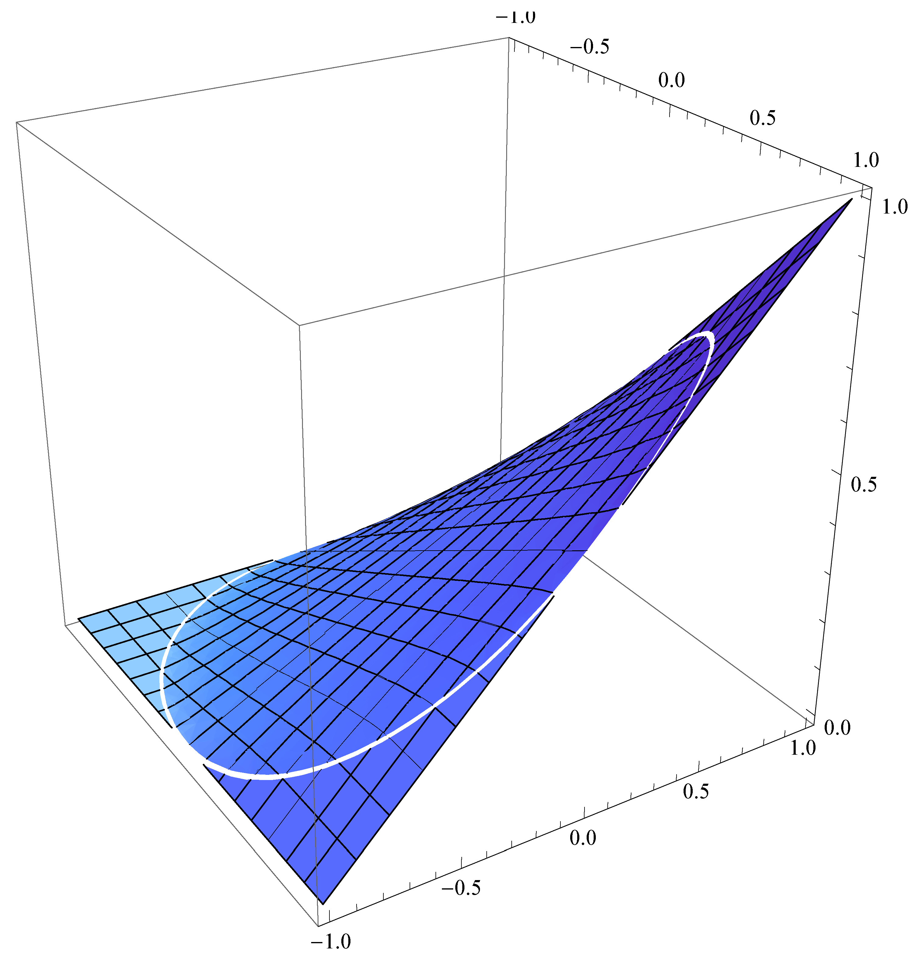
Figure 8 shows the density
with
.
To describe the family of elliptical copulas
, we extend the definitions (
16) and (
18) as follows. First, for
define
Note that
reduces to
in (
16) when
,
i.e., when
. From (
12),
Next, extend the definition of
to
as follows (see
Figure 9):
Note that (
34) and (
36) agree on
,
i.e., when
. Also note that (
36) reduces to
in (
18) when
. The following lemma will be useful for the proof of Theorem 5.1.
Lemma 5.1. Let be a bivariate random vector in with uniform marginals that satisfies . Then the cdf satisfies Proof. By the symmetry condition,
□
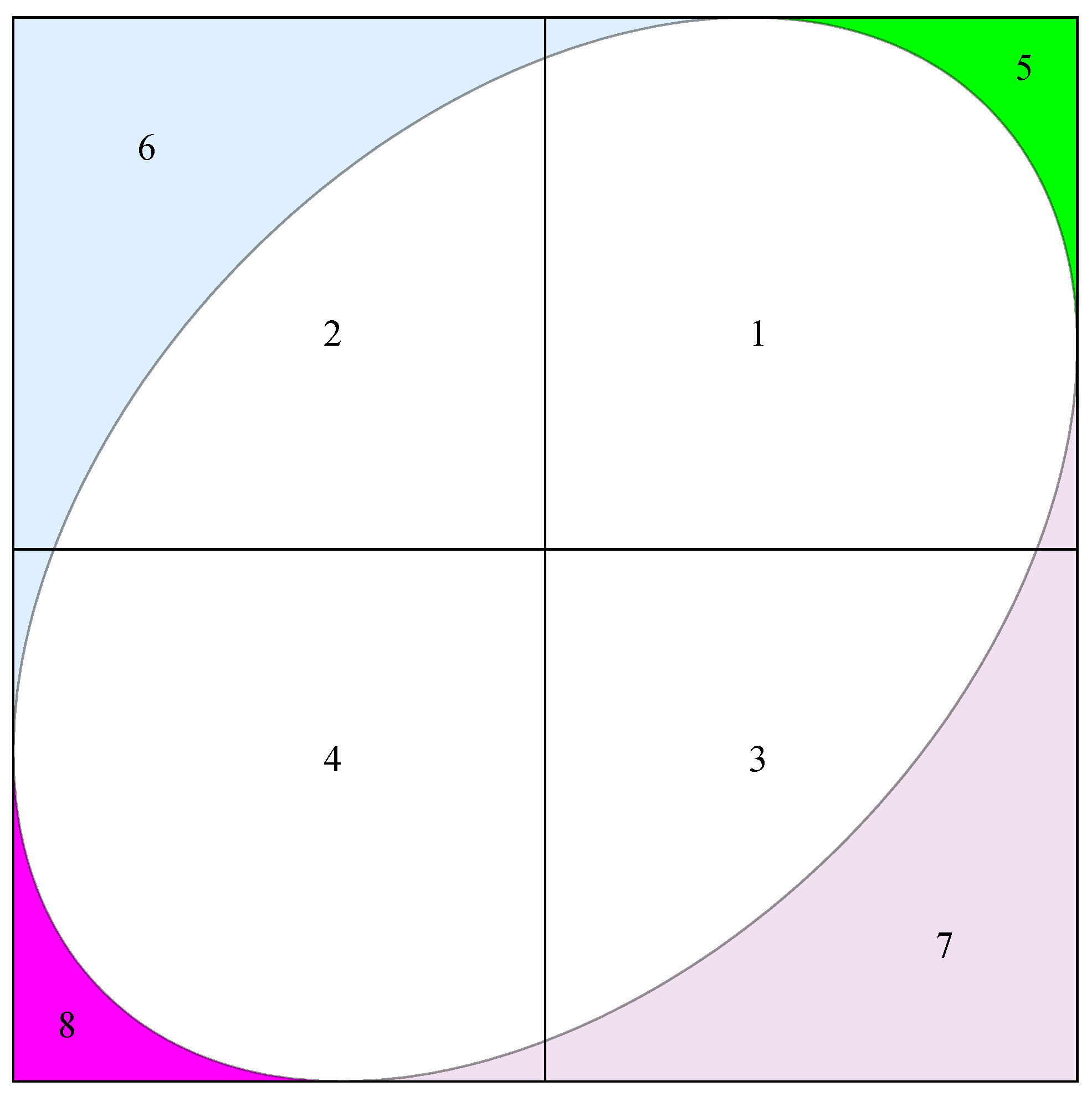
Theorem 5.1. The cdf ≡ copula of is given by (see Figure 12) Proof. To find
we again use the formula (
12) for the area of the intersection of two spherical caps on
. Here, unlike (14), the axes of the two caps are not necessarily perpendicular. The single formula (
38) is obtained by considering the partition
, where
are defined in (
36) and (see
Figure 9)
Case 1: . By using
Figure 10,
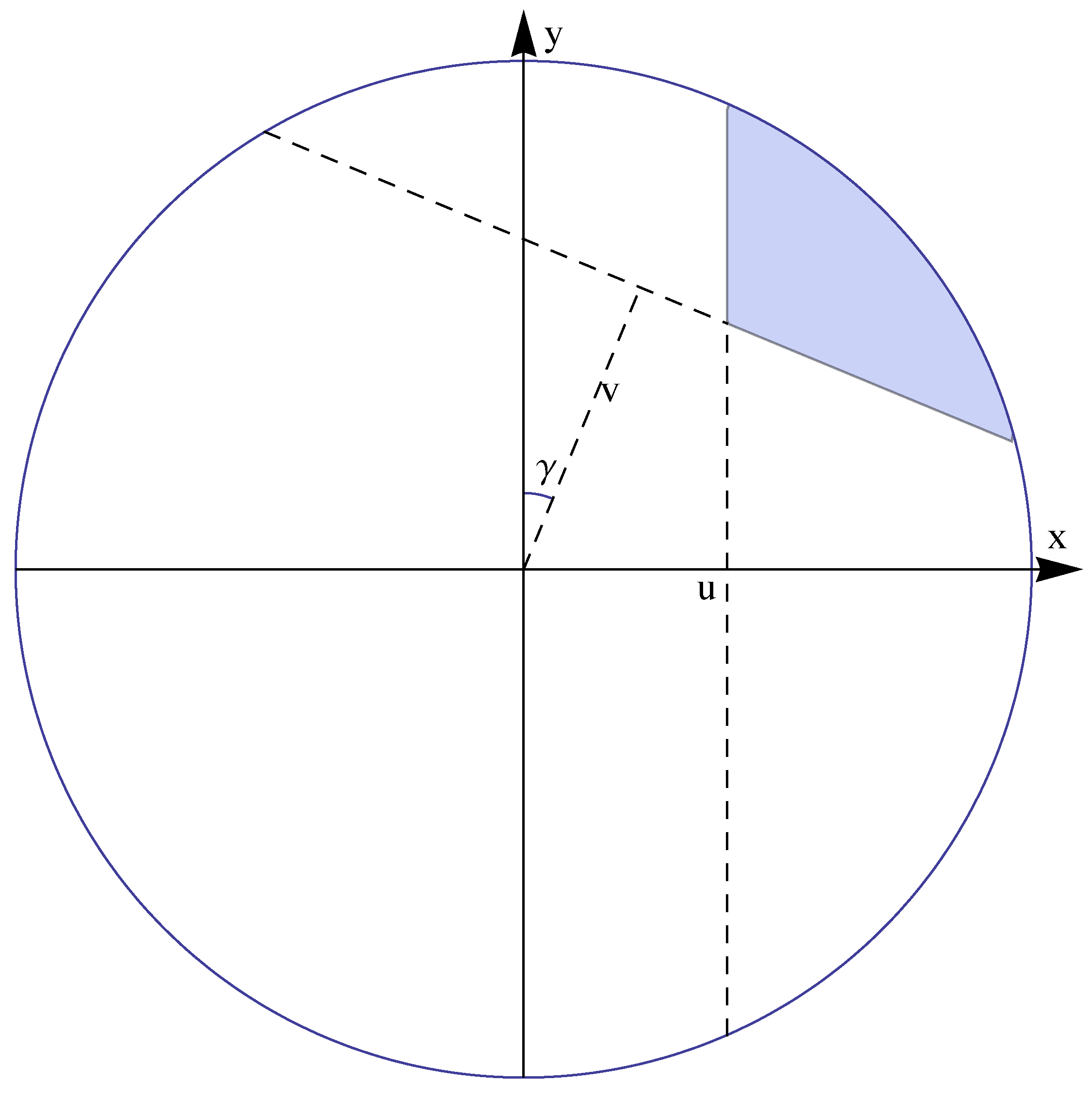
Case 2: . Because
and using
Figure 11 Case 3: . Then
, so by Lemma 5.1 and Case 2,
Case 4: . Then , so by Lemma 5.1 and Case 1, the argument for Case 3 applies verbatim.
Case 5: .
Case 6: .
Case 7: . Then , so by Lemma 5.1 and Case 6, the argument for Case 3 applies verbatim.
Case 8: . Then , so by Lemma 5.1 and Case 5, the argument for Case 3 applies verbatim. □
6. Copulas Derived from the Uniform Distribution on the Unit Ball
Up to now we have addressed the question of whether copulas can be generated by means of linear functions of a circularly symmetric or spherically symmetric random vector. Now we ask whether non-linear functions of such random vectors can generate copulas. We shall restrict attention to random vectors uniformly distributed over the unit ball and produce relatively simple non-linear functions that generate copulas on .
We begin with the bivariate case. Suppose that
is distributed uniformly on the unit disk
. Because
it follows that the random variables
satisfy
Thus,
U and
Y are independent,
V and
X are independent, and unconditionally,
so the joint distribution of
generates a copula
on the centered cube
. Note that
U and
V are not linear functions of
.
Question 6: Are U and V independent, and if not, what is the nature of their dependence?
Answer: Clearly
U and
V are uncorrelated, since
and
all by the circular symmetry of
. However, the joint pdf and cdf of
derived below show that they are not independent.
Proposition 6.1. The joint density of is given by (see Figure 13) Proof. This pdf is again obtained via the Jacobian method. It follows from (
39) that
Substitution of the second expression for
into the left side of the first relation and vice versa yields
so, since
x and
u (
y and
v) have the same signs by (
39), we obtain
By symmetry it follows that the Jacobian is given by
and hence the determinant of
J is given by
Because the pdf of
is
, the result (
40) follows. □
For
,
, let
and
be the ellipses
The next lemma leads to the cdf
corresponding to the pdf (
40).
Proof. Define the points
as follows: see
Figure 14,
Then
from which the result follows. □
Theorem 6.1. The copula (= cdf) corresponding to the pdf (40) is given by (see Figure 15) Proof. Because
is sign-change invariant and has uniform
marginals, it follows from (
7) and (
9) in Lemma 3.1 and from (
39) that for
,
The result now follows from Lemma 6.1. □
Remark: The construction (
39) extends readily to generate a copula on
. For
, for example, let
be uniformly distributed on the unit ball
and define
Then the marginal distributions of
U,
V, and
W are each uniform
so the cdf
is a copula on
. To find this copula one would need to determine
, where now, for
,
,
, and
are the ellipsoids
