A Design Approach for Mei Gui Chairs Based on Multimodal Technology and Deep Learning

Abstract

Understanding the influence of the morphological mechanisms of Mei Gui chairs on the emotional preferences of female users is crucial for achieving perceptual resonance in design. This study aims to investigate/explore the relationship between user preferences and design features to create furniture with greater emotional resonance. (1) Background: To develop a scientifically validated model for predicting user preferences in Mei Gui chair design by emotional factors and morphological mechanisms. (2) Methods: (a) Data Collection: Establish a dataset of Mei Gui chair morphological mechanisms based on the visual sequences of female users using the KJ method, factor analysis, K-means clustering, and triangular fuzzy numbers. (b) Preference Analysis: Use Eye-tracking Technology to identify female users’ preference areas for Mei Gui chair morphology and construct a morphological element preference library. (c) Feature Classification: Categorize the extracted feature elements into five classes. (d) Neural Activation Analysis: Utilize near-infrared brain functional imaging technology to conduct paired-sample T-tests on the five classes of features, identifying preferred backrest characteristics. (e) Model Validation: Integrate three factors (elegance, delicacy, comfort) into the final design scheme and compare the performance of the proposed EMD-KPCA-LSTM model with traditional BP neural network, SVM, and CNN models. (3) Results: The EMD-KPCA-LSTM model outperforms traditional models in capturing the relationship between user preferences and morphological mechanism design features, demonstrating higher predictive accuracy, better generalization ability, and stronger robustness. (4) Conclusions: The proposed model effectively integrates user preferences with Mei Gui chair design, providing a scientifically validated method for perceptual prediction in furniture design.

1. Introduction

In Chinese traditional culture, the Mei Gui chair, or “lady’s chair,” was historically crafted for upper-class noblewomen. Its design incorporates specific ergonomic considerations: a shallow seat facilitates graceful sitting suited to traditional women’s attire (such as long skirts), a moderate backrest height provides support without interfering with elaborate hairstyles, and curved armrests align with the natural posture of the arm. These features reflect the humanistic care embedded in traditional furniture. The recent revival of such furniture in contemporary homes represents a cultural renaissance, merging heritage preservation with modern esthetics.

This focus on a specific user group is rooted in documented history and craft tradition, avoiding simplistic generalizations. However, designers now face a critical challenge: reconciling historical design language with personalized preferences in an era of mass customization, driven by both market growth (the Chinese home furnishing market’s CAGR was 6.8% from 2019 to 2024 [1]) and the demand for emotional design.

In emotional design, Kansei Engineering (KE) provides a framework for translating user emotions into product features. Yet, traditional KE often relies on subjective designer experience for “morphological decomposition,” lacking objective, quantifiable definitions. This subjectivity hinders precise modeling and reproducible verification.

To address this gap and better understand female preferences for the Mei Gui chair, this study introduces a quantifiable morphological decomposition method:

(1)

Curvature: Key contours (e.g., of the armrest) are analyzed for average curvature and change rate (mm⁻¹) to quantify fluidity.

(2)

Angles: Angles between components (e.g., backrest and seat) are measured in degrees (°) to assess proportion and structure.

(3)

Pixel Share: The relative area of components (e.g., carved panels) within frontal images is calculated to quantify visual weight and decorative complexity.

The consistency of these measurements was validated via inter-rater reliability assessment, with experts measuring samples and a high intraclass correlation coefficient (ICC) confirming methodological reliability [2].

Beyond objective morphology, this study employs multimodal data fusion for deeper preference analysis. Recent research highlights its potential: used EEG and eye-tracking to predict consumer preferences [3]; combined EEG and eye-tracking for remote object detection, shedding light on cognitive processes [4]; others have used fNIRS for brain activity analysis [5] or combined it with EEG for improved emotion recognition [6].

Building on these advances, our study integrates the chair’s morphological parameters, eye-tracking, and fNIRS. This captures the design stimulus, visual attention, and neural response simultaneously. Eye-tracking identifies preferred design regions through fixation and scan-path analysis [7]. Concurrently, fNIRS measures cortical oxygenation changes (HbO/HbR), reflecting emotional and cognitive states linked to specific design elements.

To analyze this integrated data, we employ an EMD-KPCA-LSTM model. This model excels in complex time-series prediction. First, Empirical Mode Decomposition (EMD) extracts multi-scale features from the data as Intrinsic Mode Functions (IMFs), a method proven across fields [8,9]. Kernel Principal Component Analysis (KPCA) then reduces the dimensionality of these IMFs, capturing nonlinear relationships and mitigating overfitting risk. Finally, a Long Short-Term Memory (LSTM) network processes the refined data to model long-term dependencies.

The specific contributions of this study are threefold:

(1)

A Quantified Morphological-Preference Database: We integrate Kansei Engineering methods with objective morphometrics and eye-tracking, creating a database that links quantifiable geometric features of Mei Gui chairs to user visual attention, moving beyond subjective description.

(2)

Neural Validation of Design Impact: Using fNIRS, we provide neurophysiological evidence for female user preferences, identifying how specific design elements (e.g., full carvings) elicit stronger activation in brain regions related to esthetic appraisal.

(3)

A Novel Multimodal Fusion Prediction Model: An EMD-KPCA-LSTM model is proposed and validated. Tailored for heterogeneous design and physiological data, it addresses non-stationarity and high-dimensional features, and demonstrates enhanced predictive performance compared to several benchmark models (BP, SVM, CNN, LSTM).

The paper is organized as follows: Section 2 details the methodology, including morphometric quantification, multimodal data acquisition, and model construction. Section 3 presents the experimental results. Section 4 discusses the implications for design. Section 5 concludes the paper.

2. Materials and Methods

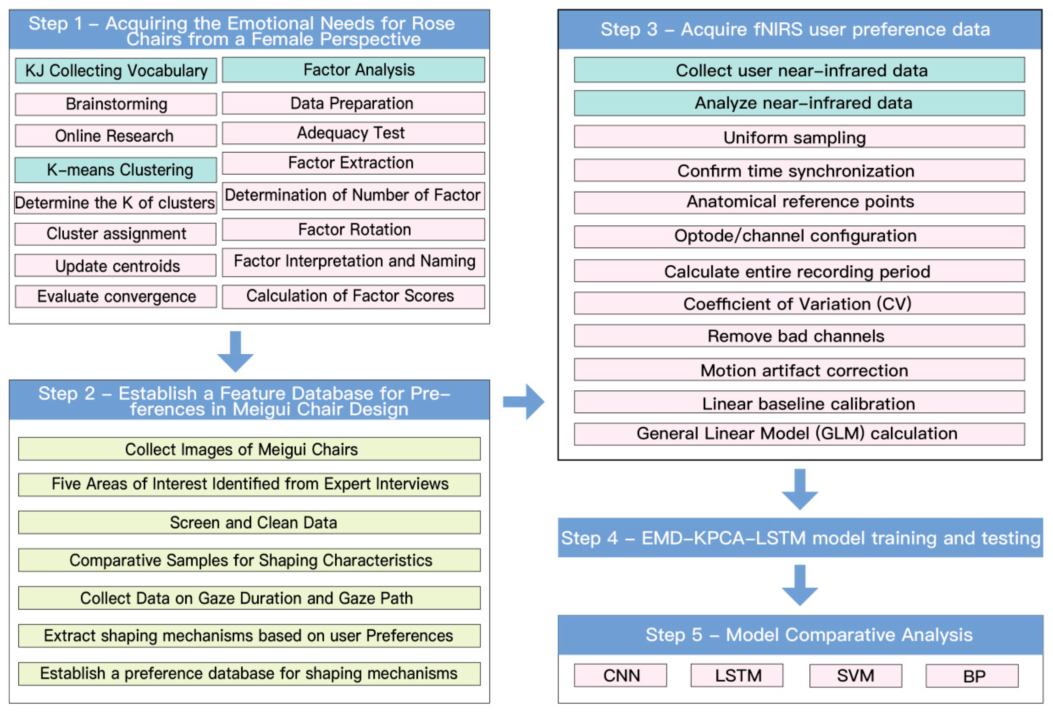
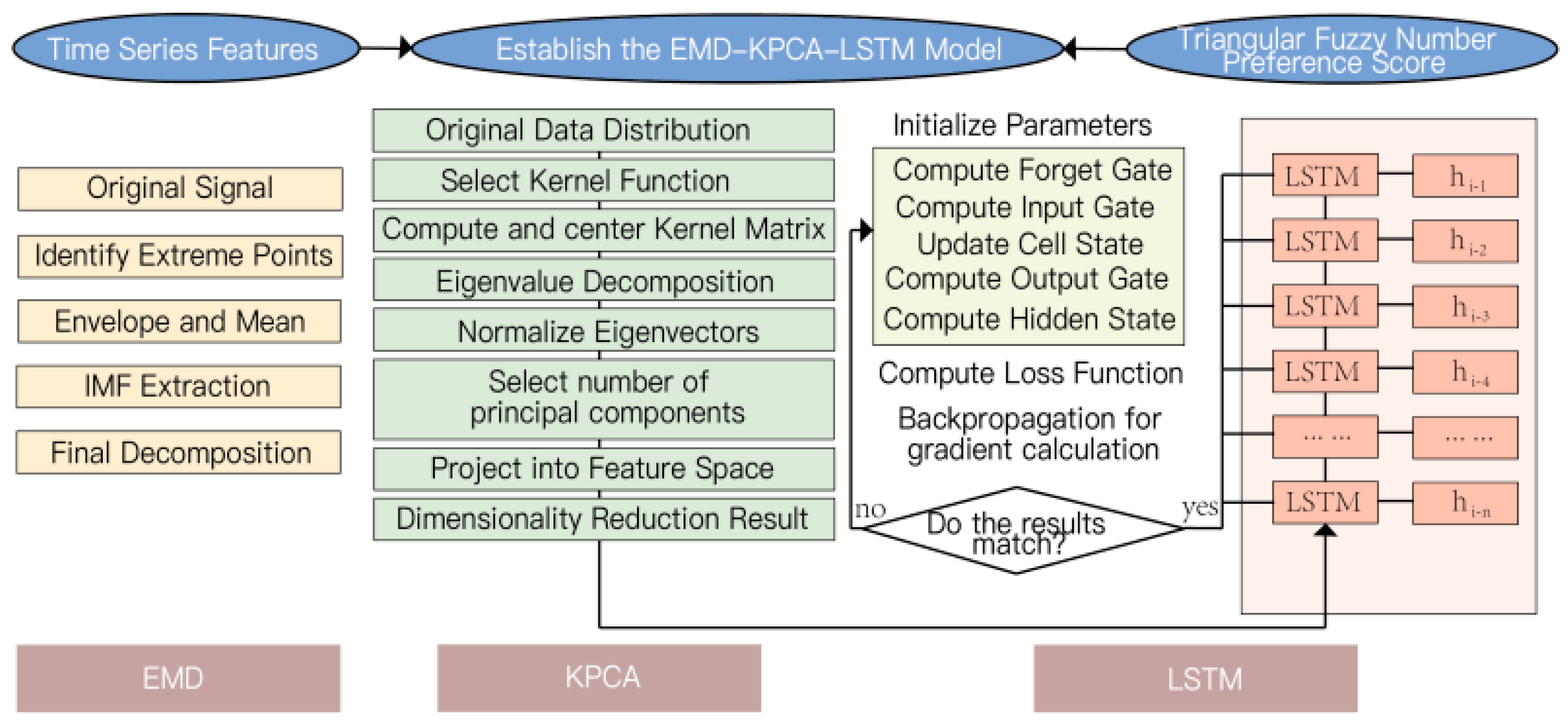
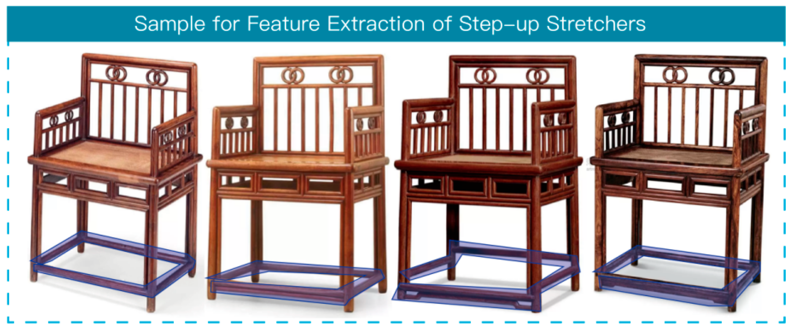
This study aims to utilize the EMD-KPCA-LSTM framework to train a dataset of visual sequences of Mei Gui (Rose) chair morphologies, with the goal of enhancing the accuracy of user preference prediction. Furthermore, this research seeks to construct a mapping model between the morphological features of Mei Gui chairs and user emotions, thereby designing Mei Gui chairs that align with user preferences. The specific research process is outlined as follows:

Step 1: Employ the KJ method to acquire descriptive vocabulary for Mei Gui chairs, followed by K-means clustering to group the data. Factor analysis is then applied to extract and name user preference factors [10].

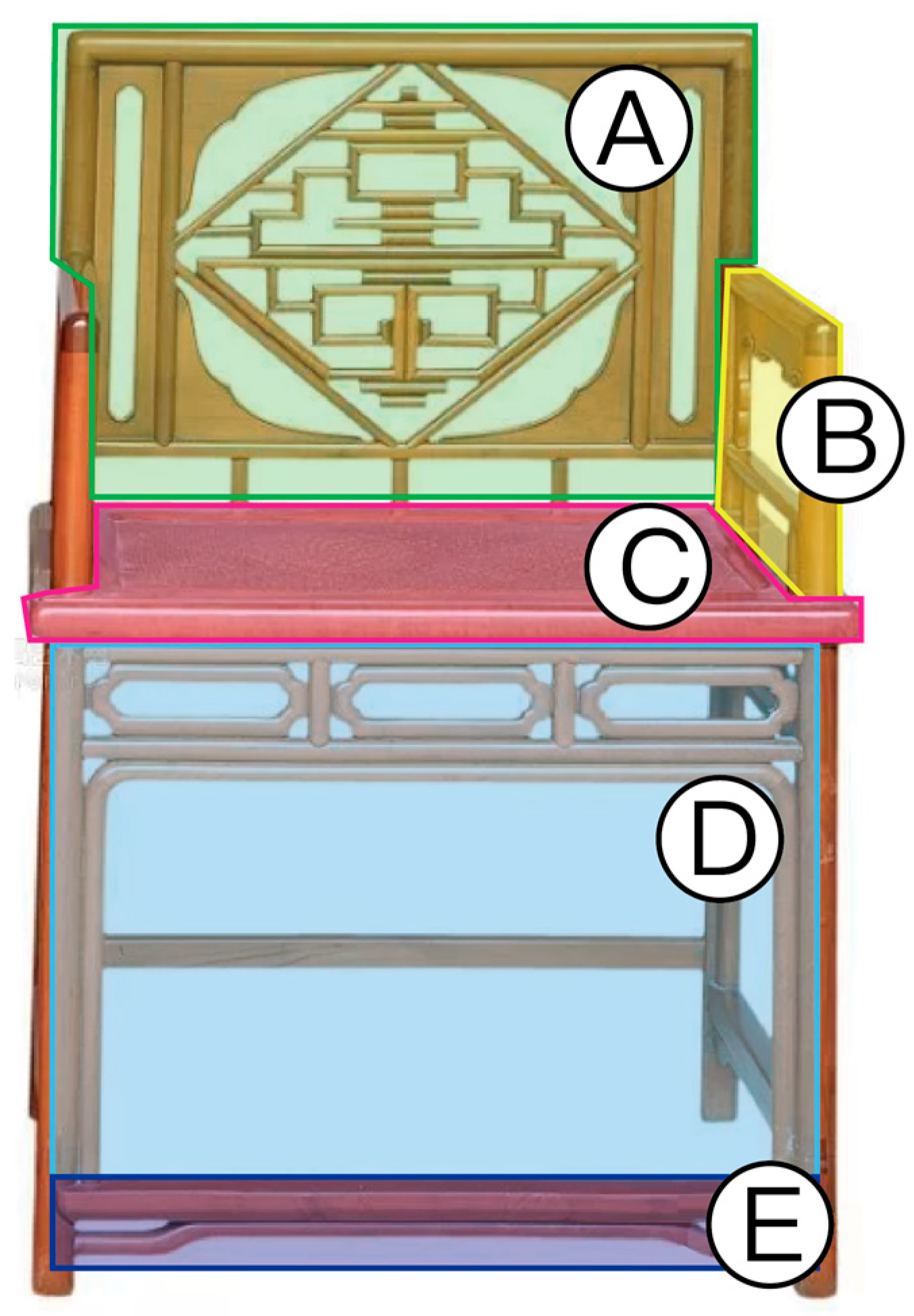
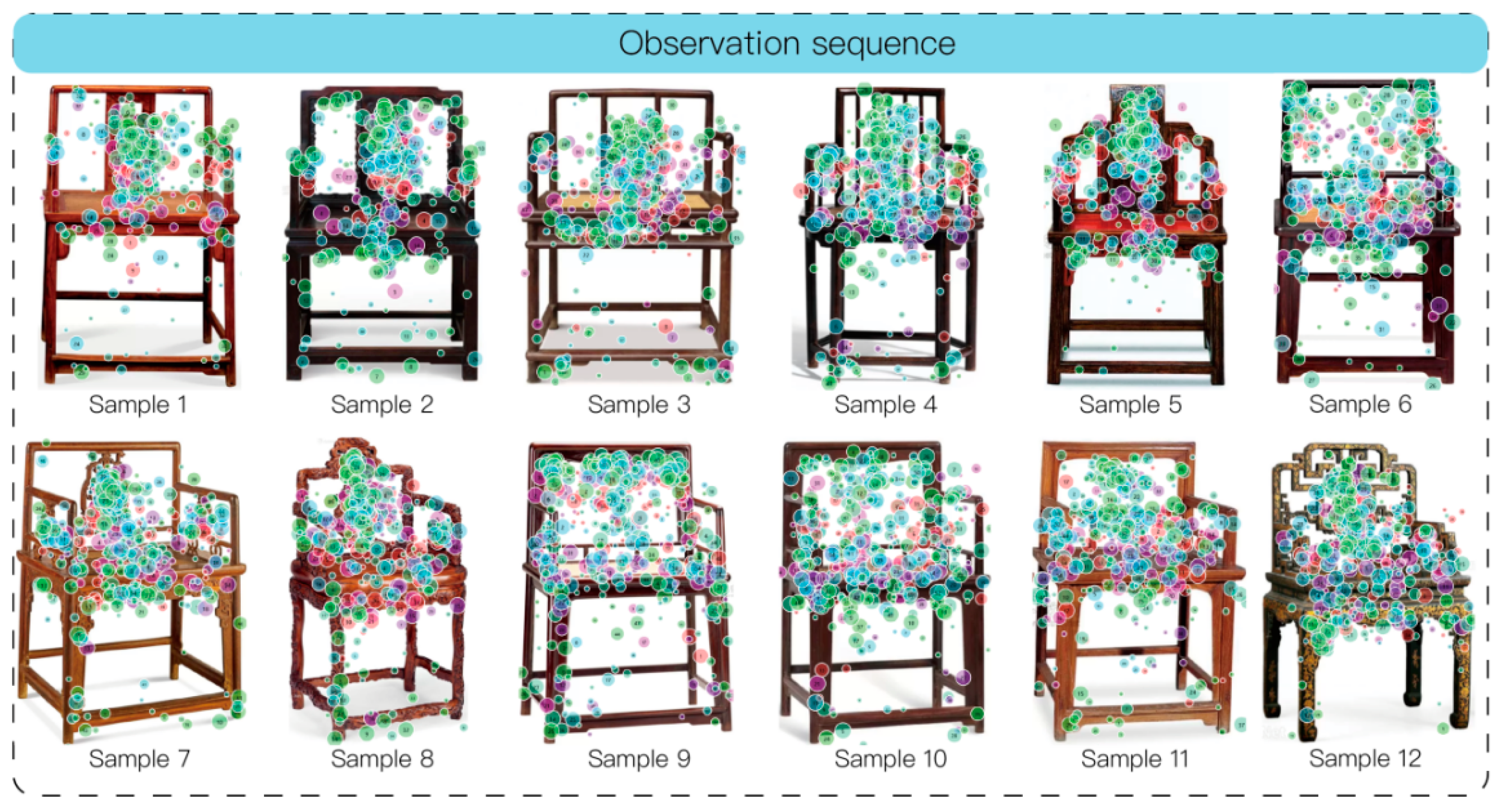
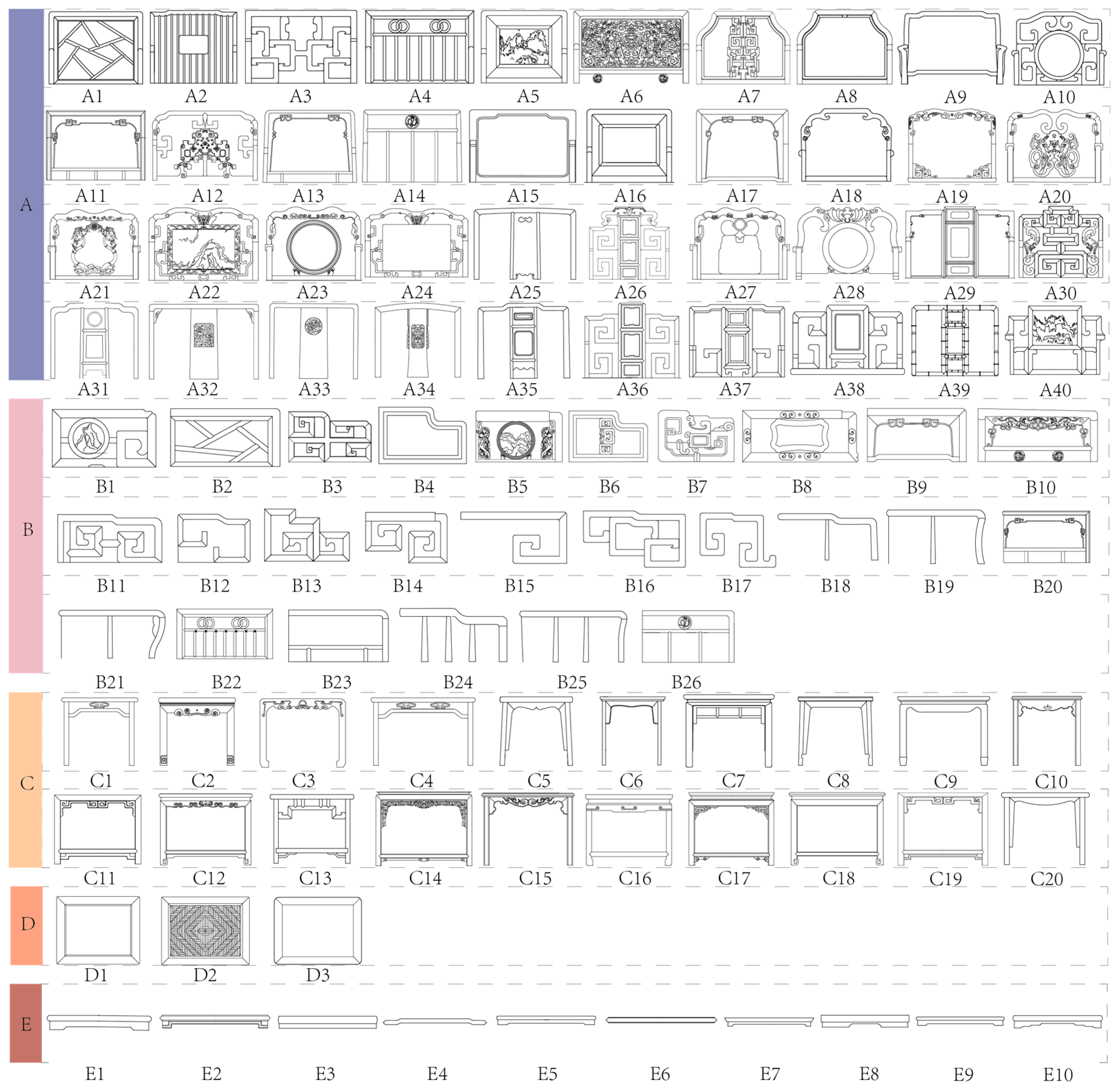
Step 2: Collect high-resolution images of Mei Gui chairs. Through expert interviews, partition the morphological mechanisms into regions to establish a comparative sample map of element preferences. Collect eye-tracking data from experts to create a design element table for user-preferred Mei Gui chair forms. Simultaneously, collect preference evaluation scores from female users for each Mei Gui chair design, which are subsequently transformed using triangular fuzzy numbers.

Step 3: Acquire and process functional near-infrared spectroscopy (fNIRS) data. The fNIRS device used was the NirSim-100 wearable functional near-infrared brain imaging system from Wuhan Yirui Technology Co., Ltd. (Wuhan, China).

Step 4: Input the obtained eye-tracking data and user evaluations into the established EMD-KPCA-LSTM model for training.

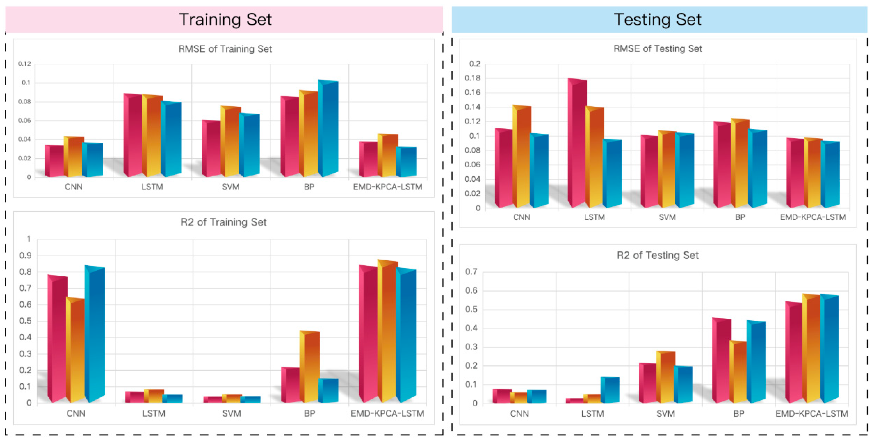
Step 5: Input the data into traditional frameworks such as CNN, SVM, and BP, and compare the results with simpler benchmark models (e.g., KPCA + SVM, Random Forest) to comprehensively evaluate the effectiveness of the proposed framework.

The detailed procedure is illustrated in Figure 1. This structured approach ensures a comprehensive analysis of user preferences and facilitates the development of Mei Gui chair designs that resonate with the target audience.

2.1. User Data Collection Process

This study collected visual sequence data and fNIRS data from 35 female participants. The experimental design was structured as follows:

(1)

Sample Selection

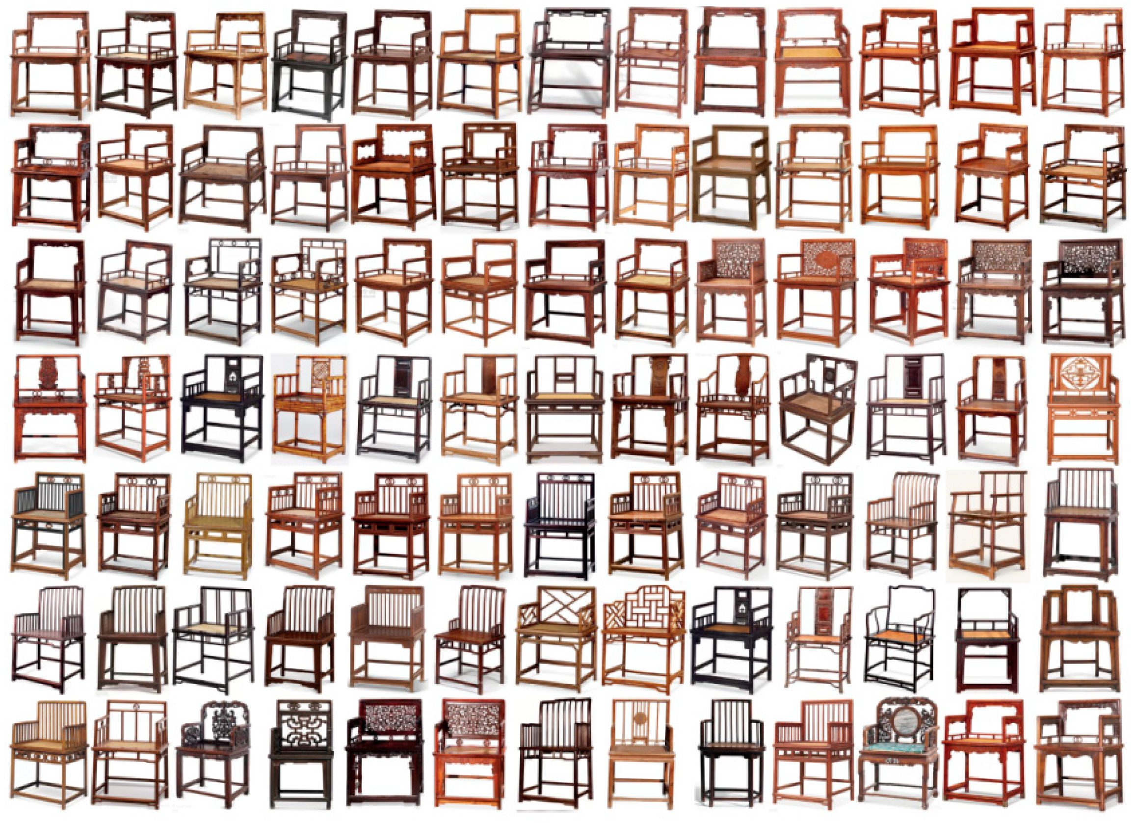
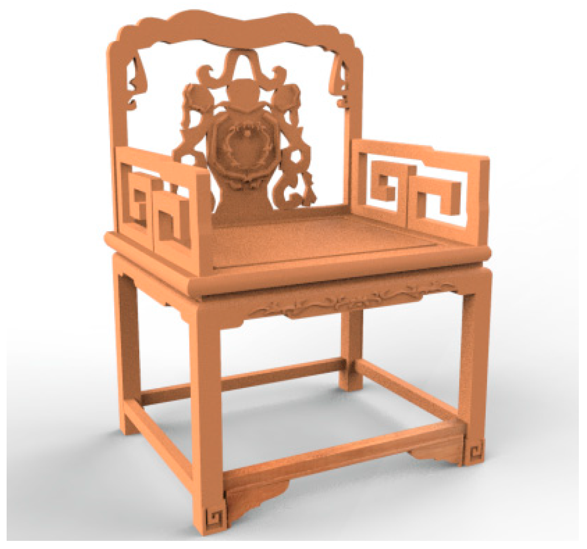
A total of 94 images of Mei Gui chairs, representing the key characteristics of the dataset, were selected. The resolution and viewing angle of all stimulus samples were standardized. Based on the structural design components of the Mei Gui chair, five categories of morphological features were identified, corresponding to pre-defined Area of Interest (AOI).

Clarification on Sample Selection Criteria: The 94 images were selected from an initial pool of over 200 historical and contemporary Mei Gui chair images. The selection criteria included the following: (1) Era Representativeness: covering three main periods: Ming-style (minimalist), Qing-style (ornate), and modern innovative designs; (2) Craftsmanship Style: balanced selection of representative works from five major craftsmanship and decoration styles: Plain Carving, Comb-Back Chair, Narrow Backrest, Hollow Backrest, and Full Carving; (3) Morphological Integrity: ensuring images were high-definition (resolution no less than 1920 × 1080 pixels), frontal view, and with unobstructed main subjects; (4) Material Visibility: images needed to clearly show wood grain (e.g., rosewood, padauk, wenge wood) and any possible metal fittings. The final selected samples were balanced across style categories to ensure diversity and representativeness of the dataset.

(2)

Participants

We recruited 35 participants, comprising 14 industry experts (including 5 designers from traditional furniture enterprises, 5 traditional furniture craftspeople, and 4 university professors in furniture design), 8 traditional furniture enthusiasts, and 13 amateur users planning to purchase traditional furniture. During the collection of visual sequence data, participants were instructed to evaluate the images using a 7-point Likert scale. The demographic characteristics of the participants are presented in

Table 1. Participant Demographic Information.

Demographic Characteristic	Category	Number (n = 35)	Percentage (%)
Age Range	18–25 years	8	22.9
	26–35 years	15	42.9
	36–50 years	10	28.6
	Above 51 years	2	5.7
Education Background	Bachelor’s Degree	18	51.4
	Master’s Degree	12	34.3
	Doctoral Degree	5	14.3
Art/Design Training	Formal training (Design major/Professional qualification)	17	48.6
	No formal training, but long-term interest	10	28.6
	No relevant training or specific interest	8	22.9

.

Supplement on Specific Scale Questions: Participants rated each Mei Gui chair image on the following four dimensions (1 = Strongly Disagree, 7 = Strongly Agree):

Esthetic Appeal: “I find this chair visually appealing.”

Perceived Comfort: “This chair looks comfortable to sit in.”

Craftsmanship Recognition: “I think the craftsmanship of this chair is of high quality.”

Purchase Intention: “If circumstances allowed, I would consider purchasing this chair.”

For the purpose of constructing machine learning models, each “participant × image” combination was treated as an independent observation. The raw data comprised a total of 35 participants × 94 images = 3290 trials. For each trial, corresponding eye-tracking and fNIRS features were extracted to form a feature vector. Therefore, each observation corresponds to the response features and multi-dimensional ratings from a specific participant for a specific image, resulting in a final dataset size of N = 3290 rows. During the subsequent model training and evaluation employing 5-fold cross-validation, a subject-based data splitting strategy was strictly implemented. This ensured that all data from the same participant (i.e., their corresponding 94 rows of observations) were always assigned to the same subset (either training or test set) in each validation fold, thereby preventing data leakage and overfitting, and guaranteeing the reliability of the model generalization assessment.

To address potential biases arising from differing levels of expertise, data from expert users (n = 14) and non-expert users (n = 21) were subjected to comprehensive analysis, subgroup analysis, and robustness checks.

(3)

Equipment

The experiment utilized an Ergolab eye-tracking system (Tobii X60/X120) with its accompanying Tobii Pro Lab software (version 24.21), (The eye-tracking data were collected and processed using Tobii Pro Lab software (developed by Tobii Pro AB, Danderyd, Sweden).) a wearable functional near-infrared brain imaging device (NirSim-100), E-Prime 3.0, and MATLAB 2023a.

(4)

Experimental Procedure

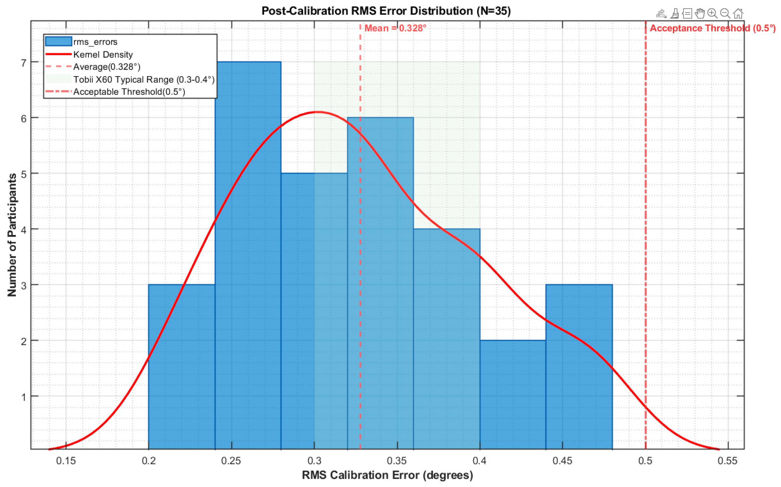
Following an introduction to the experimental workflow, participants underwent a standardized calibration and adaptation phase to ensure data validity. Calibration was performed using a nine-point grid procedure, wherein participants were instructed to sequentially fixate on red dots (diameter: 0.5° visual angle, duration: 1500 ms) displayed at predetermined positions on the screen, maintaining a viewing distance of 60 cm.

Calibration accuracy was validated through a two-step process: (1) The gaze deviation for each calibration point was required to be less than a preset acceptance threshold of 0.5° (this threshold is stricter than the device’s typical accuracy of 0.3–0.4° at 60 cm distance). (2) Operator monitoring and verification: The operator inspected the gaze trajectory in real time to ensure its consistency with the sequence of calibration points.

During the experiment, the wearable fNIRS headpiece was properly positioned, and channel alignment was performed prior to data acquisition using E-Prime 3.0.

Following the experiment, heat maps were generated using Tobii Pro Lab, and gaze sequence data were exported. These data were subsequently analyzed with the NirSim-100 proprietary software (V2.1).

2.2. Multimodal Technology

2.2.1. Eye-Tracking Technology

Eye-tracking technology is a non-invasive experimental tool that detects human eye movements to obtain data on attention distribution, eye movement trajectories, and gaze speed. This technology is based on the “brain-eye consistency hypothesis,” which posits that the location of gaze is typically related to the object of attention and thought. Currently, popular eye-tracking techniques primarily rely on video-oculographic (VOG) analysis, a non-invasive method. Its fundamental principle involves directing a beam of light (near-infrared) and a camera toward the participant’s eyes, using the light and backend analysis to infer the direction of gaze. In this study, we utilized the ErgoLAB device to capture feature data related to the design of Mei Gui chairs.

2.2.2. Functional Near-Infrared Spectroscopy (fNIRS)

The analysis was performed using the NirSim-100 software, adhering to the following procedural steps:

Data Import and Preprocessing.

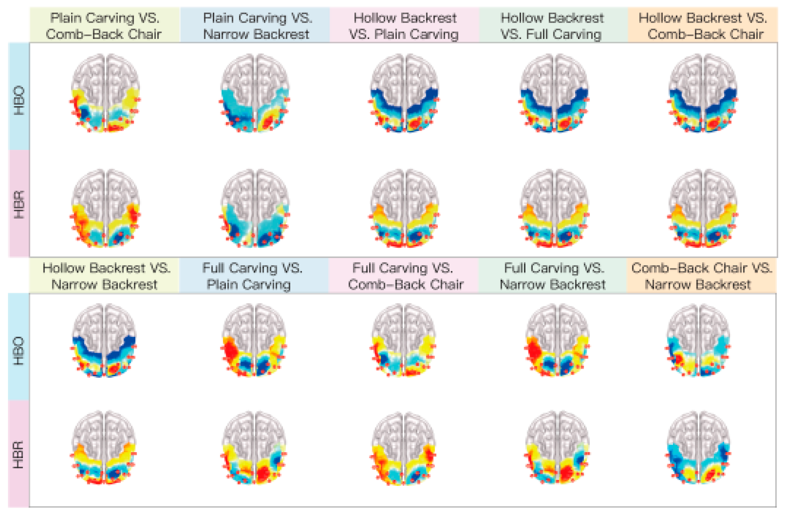
Data Import: The analyzed eye-tracking data segments were imported and categorized into five distinct groups (Plain Carving, Comb-Back Chair, Narrow Backrest, Hollow Backrest, and Full Carving), with 10 images per group, to investigate the influence of specific Mei Gui chair design types on user preferences [11].

Sampling Rate Configuration: The sampling rate was set to 20 Hz, consistent with the data acquisition parameters [12].

MARK Time Validation: The accuracy of the pre-configured MARK timestamps was rigorously validated. These markers correspond to the onset of the 1200 ms chair image presentation period within each trial.

Spatial Registration: Anatomical reference points and the optode channel layout were input. Brain region mapping was subsequently performed by selecting the Brodmann area map and the Automated Anatomical Labeling (AAL) atlas.

Quality Control: Channel-wise CV Calculation: The coefficient of variation (CV) was computed for the entire dataset, with time zero as the starting point. The bad channel threshold was established at 15%. This specific threshold was determined via Bonferroni correction: given the 20 Hz sampling rate and a 1.2 s trial duration, each channel generated 24 time points per trial. Considering the number of channels (N = 22) in the equipment used, the conventional 20% threshold was adjusted to a more stringent level (α = 0.05/N channels) to control the family-wise error rate, thereby deriving the practical CV threshold of 15%. (This value could be directly calculated and selected within the experimental apparatus software).

Block-wise CV Calculation: The CV was calculated for each individual trial, using the MARK onset as time zero. The start time was set to −200 frames (to preserve the baseline period), and the end time was set to 1200 frames (representing the stimulus presentation duration minus the baseline period). The bad channel threshold for this block level assessment was set at 20%.

Data Preprocessing: Motion Artifact Correction: Motion artifacts were corrected by applying the SPLINE interpolation method. The specific parameters employed were as follows: TmotionWEI = 0.5 (a weighting coefficient for the motion artifact time window, controlling the temporal smoothness during artifact detection), STDEVthresh = 20 (the signal standard deviation threshold, where signal fluctuations exceeding this value were identified as potential motion artifacts), TMASK = 3 (the duration for masking artifacts, used to mark and overwrite continuous data segments identified as artifacts), and AMPTHRESH = 5 (the signal amplitude threshold, where abrupt signal changes exceeding this amplitude were detected as motion artifacts) [13].

Evaluation of Motion Artifact Correction Efficacy: To assess the impact of SPLINE interpolation on signal quality and to rule out the potential introduction of spurious activation, power spectral analysis was conducted on the oxygenated hemoglobin (HbO) concentration change signals, both before and after correction. Figure 2 illustrates the power spectral density (PSD) for a representative channel, pre- and post-interpolation.

Figure 2 depicts the HbO power spectrum: the short-distance channel (serving as the reference channel dominated by motion artifacts) exhibited significantly lower PSD in the 0~2 Hz frequency band compared to the long-distance channel (the tissue signal channel) and the corrected curve. This indicates that the original long-channel signal contained elevated power components induced by motion artifacts. The high concordance between the post-correction HbO power spectrum (green curve) and the long-channel spectrum (blue) demonstrates that SPLINE interpolation effectively mitigated the power interference from motion artifacts without introducing substantial additional spectral components.

Figure 2 shows the HBR power spectrum: the corrected curve (purple) and the long-channel curve (blue) showed good consistency in PSD within the 0~2 Hz range, while the short-channel power remained markedly lower. This further validates the efficacy of the correction in suppressing motion artifacts. The absence of anomalous power peaks or extra frequency components in the post-correction spectra suggests that SPLINE interpolation did not introduce significant spurious frequencies or power components, indirectly reducing the risk of false activation. Across all datasets, segments requiring interpolation correction accounted for 5% of the total data volume. In the context of task-based data, this low percentage indicates generally good overall data quality, and the minimal interpolation further diminishes the likelihood of false activation.

Detrending: A linear detrending algorithm was applied to remove linear trend components from the signals, which typically arise from instrumental drift or slow physiological fluctuations (e.g., respiration, heart rate baseline wander).

Block Averaging: Accounting for the inherent data acquisition delay of the equipment, the temporal window for each stimulus-locked signal block was defined from −200 frames (pre-stimulus onset, preserving the baseline) to 1200 frames (the effective stimulus presentation period, constituting the signal interval after baseline subtraction). Furthermore, based on the Coefficient of Variation (CV) results, data blocks labeled as ‘bad segments’ (indicating substandard signal quality) were excluded from subsequent averaging.

Baseline Correction: Baseline correction was performed using a linear fitting approach. The baseline time interval was defined from −2 s to 0 s relative to stimulus onset (i.e., the 2 s period immediately preceding stimulus presentation was used as the baseline for calibrating the relative signal changes post-stimulus).

2.3. EMD-KPCA-LSTM Model

This study collected 94 sample data points from 35 participants. The raw feature dimension was 8, comprising multimodal eye-tracking and fNIRS data. The target variable was the user’s preference rating on a 7-point Likert scale [14,15].

Model Input Features: The eight features are as follows: (1) Total Fixation Duration, (2) Number of Fixations, (3) Average Fixation Duration, (4) Saccade Path Length, (5) Pupil Diameter Change, (6) Mean Oxygenated Hemoglobin Concentration (Δ[HbO]), (7) Mean Deoxygenated Hemoglobin Concentration (Δ[HbR]), and (8) Brain Activity Asymmetry Index (the difference in average Δ[HbO] between the left and right prefrontal cortex). These features were calculated for each trial (each participant viewing each image) to form the model’s input vector [16].

Data Splitting and Validation Strategy: Two validation strategies were employed to ensure robust model evaluation:

(1)

Subject-Based Stratified 5-Fold Cross-Validation: The 35 participants were randomly divided into 5 folds (7 participants per fold). In each iteration, data from 4 folds (~75 samples) were used for training, and the remaining fold (~19 samples) was used for testing [17]. This process was repeated 5 times, ensuring each participant’s data was included in the test set once. Performance metrics are reported as the mean ± standard deviation across the 5 folds, serving as the primary evaluation method.

(2)

Hold-Out Independent Test Set: An additional random split allocated 75% of the data for training and 25% for testing. This set was used to demonstrate the final model’s performance after hyperparameter tuning and for comparison with commonly used methods in the literature. All hyperparameter optimization was performed on the training folds of the cross-validation [18,19].

Data were normalized using Z-score normalization, with the mean and standard deviation calculated from the current training fold.

2.3.1. Empirical Mode Decomposition (EMD)

Empirical Mode Decomposition (EMD) is employed to decompose the complex temporal evolution of affective preferences into Intrinsic Mode Functions (IMFs) across different time scales [20]. Within the theoretical framework of this study, we propose an interpretative hypothesis: the different IMF components obtained from the decomposition may correspond to distinct levels of cognitive and affective responses [7]. 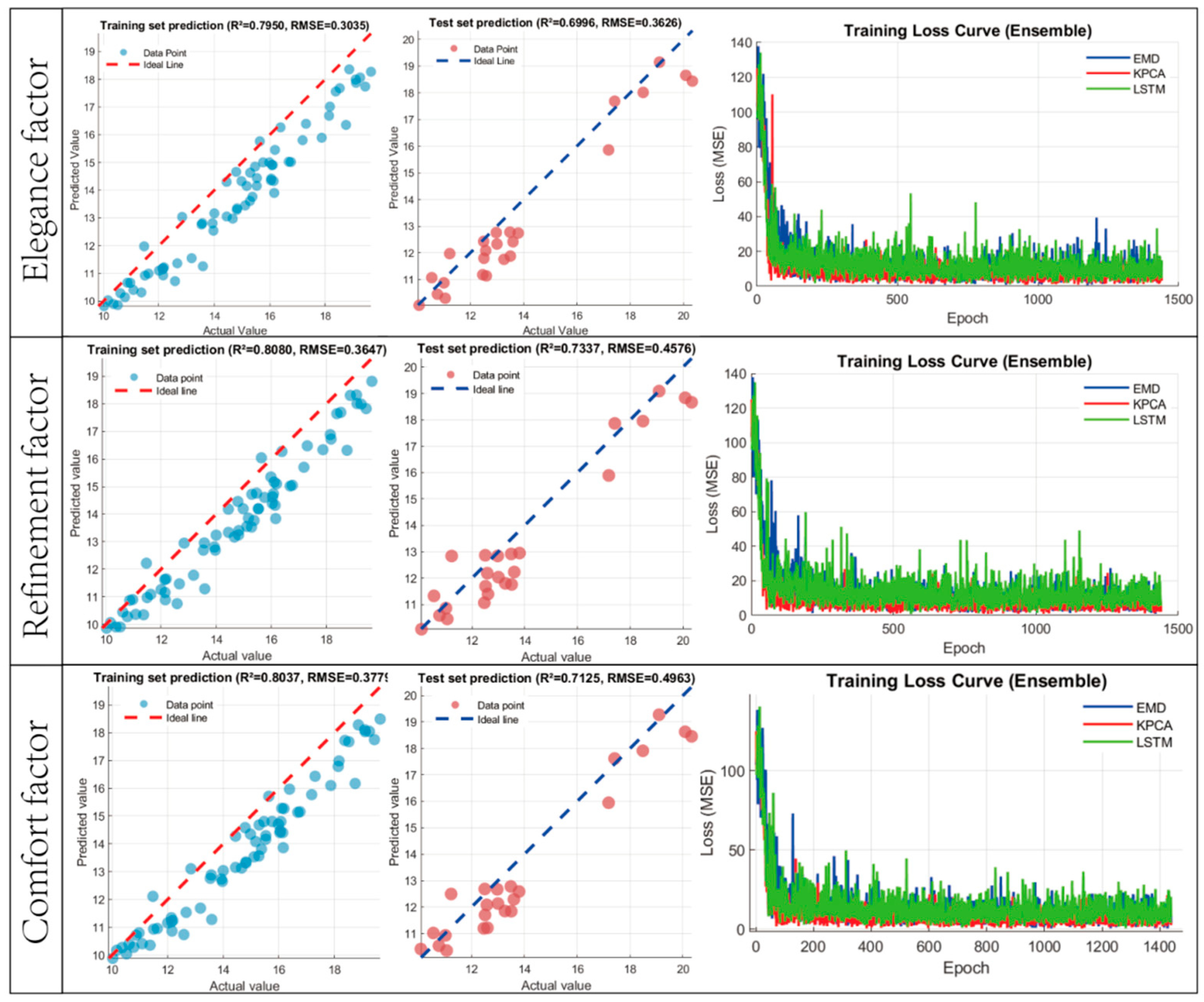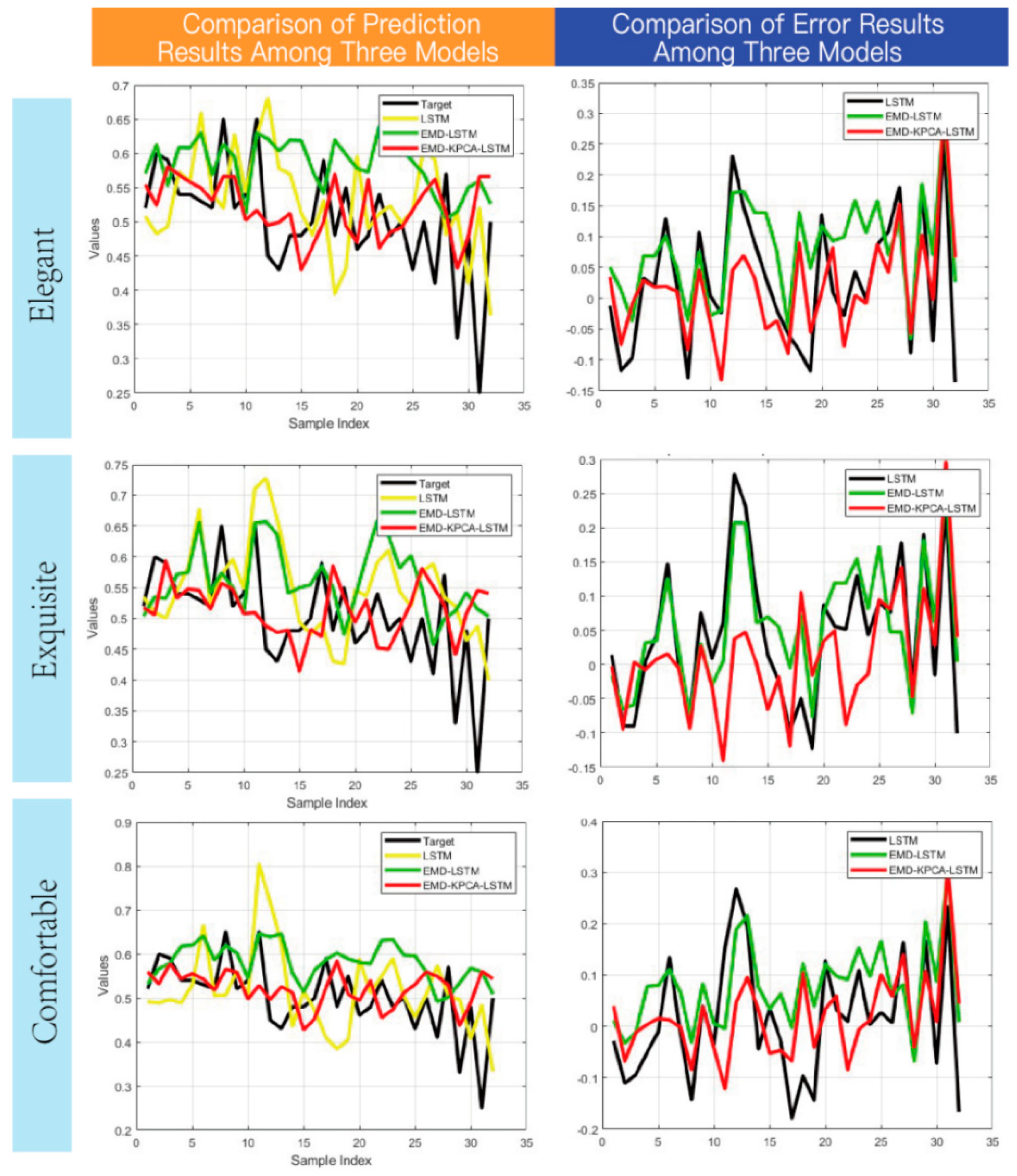Specifically, high-frequency components can be interpreted as reflecting immediate emotional reactions, medium-frequency components may correspond to cognitive processing, while low-frequency components can be construed as reflecting deep-seated values and esthetic tendencies [21]. Based on this, the study attempts to conceptually associate these hierarchical levels with the three factors of Comfort, Elegance, and Refinement, respectively. [22]. Each IMF must satisfy two conditions: the number of extrema and the number of zero-crossings must either be equal or differ at most by one, and the mean of the envelope defined by the local maxima and the envelope defined by the local minima must be zero [23,24].

A zero-padding strategy was applied during decomposition to align IMF components of variable lengths, primarily for its advantage in preserving phase information. The maximum number of IMFs was set to 5, and spline interpolation was used within the EMD algorithm.

EMD Parameter Details: The maximum number of IMFs was experimentally determined to be 5. Testing showed that using 5 IMFs achieved the optimal balance between reconstruction error and the physical interpretability of the components on the training set. The zero-padding strategy was implemented as follows: IMF sequences shorter than the maximum sequence length T_max were zero-padded at the end to reach T_max. This end-padding in the time domain corresponds to sinc function interpolation in the frequency domain, which better preserves the instantaneous frequency characteristics of the IMFs and avoids phase distortion compared to linear or spline interpolation. A masking mechanism was applied at the network input to ensure the padded portions did not contribute to loss calculation.

2.3.2. Kernel Principal Component Analysis (KPCA)

Emotional preference data often exhibit complex nonlinear structures, which are poorly handled by the linear assumptions of traditional PCA. KPCA addresses this by mapping the data into a high-dimensional Hilbert feature space via a kernel function, thereby transforming nonlinear relationships into linearly separable problems [25].

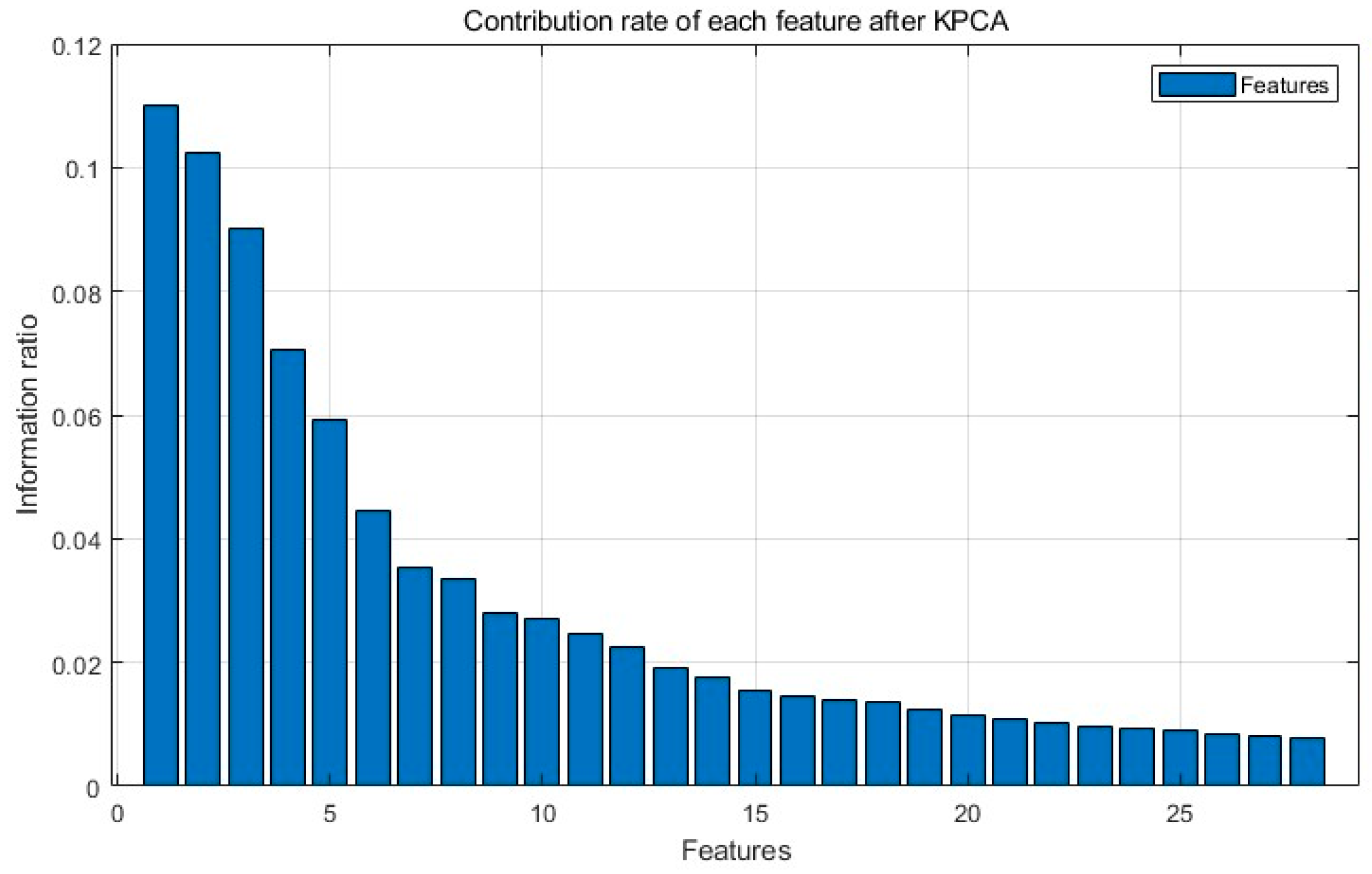
In this study, the Gaussian kernel function was selected. The kernel parameter σ was optimized to 0.5 through grid search combined with 5-fold cross-validation. The top N principal components required to achieve a cumulative contribution rate exceeding 92% were retained, effectively reducing the high-dimensional feature space to N dimensions, eliminating redundancy while preserving essential information [26].

2.3.3. Long Short-Term Memory (LSTM) Network

LSTM was used to capture long-term dependencies within emotional preference sequences [27]. Its gating mechanism effectively manages memory and forgetting effects during preference evolution: the Forget Gate controls the retention of historical preference information, the Input Gate regulates the storage of new preference inputs, and the Output Gate governs the output of the current preference [28].

An ensemble system comprising three heterogeneous LSTM sub-models was constructed, with the final output being the average of their predictions [29]. The specific configurations are as follows:

Model 1: A two-layer stacked LSTM (40 and 30 hidden units), followed by two fully connected layers (20 and 10 nodes). Dropout rates were set to 0.4, 0.3, and 0.2 sequentially [30].

Model 2: A single-layer LSTM (50 hidden units), followed by two fully connected layers (25 and 12 nodes). Dropout rates were set to 0.5, 0.4, and 0.3 sequentially.

Model 3: A single-layer LSTM (45 hidden units), followed by three fully connected layers (30, 18, and 8 nodes). Dropout rates were set to 0.45, 0.35, and 0.25 sequentially [31].

A unified training configuration was applied:

(1)

Optimizer: Adam.

(2)

Initial Learning Rate: 0.004.

(3)

Learning Rate Decay: Multiply by a factor of 0.3 every 40 epochs.

(4)

Maximum Epochs: 180.

(5)

Early Stopping: Halt training if validation loss shows no decrease for 15 consecutive epochs.

(6)

Regularization: L2 coefficient of 0.005; gradient clipping threshold of 1.

(7)

Batch Size: Adaptively adjusted between 8 and 16 based on training set size.

(8)

Loss Function: Mean Squared Error (MSE).

(9)

Random Seed: Fixed at 42 to ensure reproducibility.

2.4. Benchmark Models and Training Configuration

To validate the necessity of the EMD-KPCA-LSTM architecture, the following benchmark models were introduced for comparison:

(1)

KPCA-SVM: Original 8-dimensional features were reduced via KPCA (retaining 92% variance), followed by a radial basis function kernel SVM for regression.

(2)

Random Forest: A Random Forest regressor (100 trees) was applied directly to the original 8-dimensional features, with maximum depth determined via cross-validation.

(3)

Traditional Neural Networks: This category included a 1D CNN for sequence processing, a radial basis function kernel SVM, and a two-layer BP neural network. Inputs were either the original 8-dimensional features or EMD-decomposed feature sequences. As shown in Figure 3.

Hyperparameters for all benchmark models were optimized via grid search on the training folds of a 5-fold cross-validation.

Training Environment: All implementations were completed in MATLAB R2023a, utilizing the Statistics and Machine Learning Toolbox, Deep Learning Toolbox, and Neural Network Toolbox. The random seed was fixed using rng (42) to ensure full reproducibility.

3. Results

3.1. Data Processing Results

3.1.1. Morphological Quantification Results

To ensure the consistency and reliability of the morphological measurement data, an inter-rater reliability assessment was conducted. Fourteen experts independently measured the aforementioned morphological parameters on 30 randomly selected Mei Gui chair samples. The Intraclass Correlation Coefficient (ICC) was calculated using a two-way random-effects model. The results showed that the ICC values for all morphological parameters exceeded 0.8 (Curvature: ICC = 0.81; Angle: ICC = 0.89; Pixel Share: ICC = 0.86), indicating excellent reliability of the morphological quantification method employed in this study.

3.1.2. User Data Weighting and Validation Results

First, all participant data were screened based on the histogram of the root mean square (RMS) error after actual calibration (Figure 4), confirming that all data met the standard requirements.

To examine the potential influence of differing expertise levels, comprehensive and subgroup analyses were performed on data from both expert and non-expert participants. The comprehensive analysis did not apply differential weighting to the groups to maintain data integrity and avoid subjective bias. Concurrently, sensitivity analysis was conducted to test the robustness of a hypothetical weighting of expert data based on professional background, which showed no significant deviation from the unweighted model, confirming the stability of the findings.

Subgroup analysis revealed systematic differences in visual processing strategies between experts and non-experts, which varied across chair components. Eye-tracking data indicated that for complex components such as backrest carvings and the “Bubugaoheng” stretchers, experts exhibited significantly shorter total fixation durations, suggesting higher information extraction efficiency. For the apron and legs, the intergroup difference approached significance (p = 0.057). However, for components with relatively fixed morphology, namely armrests and the seat surface, no significant differences were observed (see

Table 2. Subgroup Analysis Results of Visual Sequence (Eye-tracking) Data.

AOI Description	Group	Mean Total Fixation Duration (s)	Standard Deviation (SD)	Statistical Test Results
AOI 1: Backrest Carving	Expert	12.5	±2.1	t = 2.15, p = 0.041
	Non-Expert	14.8	±2.9	Cohen’s d = 0.79
AOI 2: Armrest Curve	Expert	8.2	±1.8	t = 1.09, p = 0.269
	Non-Expert	8.9	±2.2	Cohen’s d = 0.287
AOI 3: Seat Morphology	Expert	6.5	±1.5	t = 0.45, p = 0.657
	Non-Expert	6.7	±1.7	Cohen’s d = 0.11
AOI 4: Apron and Legs	Expert	9.1	±2.0	t = 1.96, p = 0.057
	Non-Expert	10.8	±2.5	Cohen’s d = 0.67
AOI 5: “Step-by-Step” Stretcher	Expert	5.3	±1.2	t = 2.89, p = 0.007
	Non-Expert	6.8	±1.5	Cohen’s d = 0.91

for details). fNIRS data provided more consistent neural evidence: when evaluating backrest carvings, armrest curves, the apron and legs, and the “Bubugaoheng” stretchers, the expert group showed significantly stronger neural activation in cognitive-related brain regions such as the dorsolateral prefrontal cortex. In contrast, no significant intergroup difference was found when assessing the seat surface, which exhibits less morphological variation (see

Table 3. Subgroup Analysis Results of Neural Activity (fNIRS) Data.

AOI Description	Group	Mean HbO Concentration Change (ΔμM)	Standard Deviation (SD)	Statistical Test Results
AOI 1: Backrest Carving	Expert	0.085	±0.032	t = 2.98, p = 0.006
	Non-Expert	0.052	±0.028	Cohen’s d = 1.08
AOI 2: Armrest Curve	Expert	0.078	±0.029	t = 2.35, p = 0.026
	Non-Expert	0.055	±0.026	Cohen’s d = 0.77
AOI 3: Seat Morphology	Expert	0.045	±0.021	t = 0.89, p = 0.381
	Non-Expert	0.041	±0.019	Cohen’s d = 0.17
AOI 4: Apron and Legs	Expert	0.081	±0.030	t = 2.67, p = 0.012
	Non-Expert	0.054	±0.025	Cohen’s d = 0.89
AOI 5: “Step-by-Step” Stretcher	Expert	0.088	±0.033	t = 3.15, p = 0.004
	Non-Expert	0.050	±0.027	Cohen’s d = 1.14

for details). Together, these results indicate that the cognitive processing advantage of experts is primarily manifested when evaluating complex components rich in design semantics and craft details, rather than being universally applicable to all components.

3.1.3. Reliability and Validity Tests

Reliability and validity tests were conducted on the raw rating data from all 35 participants for the 94 samples. Reliability analysis showed that the Cronbach’s alpha coefficients for all three factors (Comfort Factor, Elegance Factor, Refinement Factor) exceeded the standard threshold of 0.7 (Comfort: α = 0.78; Elegance: α = 0.75; Refinement: α = 0.73), indicating good internal consistency reliability of the scale. Validity analysis employed confirmatory factor analysis to examine construct validity. The three-factor model demonstrated a good fit: χ²/df = 2.15, RMSEA = 0.06, CFI = 0.95, TLI = 0.93, SRMR = 0.04. All standardized factor loadings were greater than 0.6 and significant (p < 0.001), confirming that the scale possesses good construct validity.

3.2. Collection of Mei Gui Chair Samples and Preference-Emotion Vocabulary

Web crawler technology was employed to extensively collect Mei Gui Chair image samples from major traditional furniture websites, with a focus on selecting high-definition, frontal-view images. Duplicate, blurry, heavily retouched, or eye-tracking unsuitable images were subsequently removed through focus group discussions, resulting in the establishment of a Mei Gui Chair sample library as shown in Figure 5.

Simultaneously, 100 emotion-related vocabulary items associated with the Mei Gui Chair were collected (a subset is presented in

Table 4. Emotional Vocabulary Related to Mei Gui chairs (Partial).

Compact	Gentle	Elegant	Light	Agile
Exquisite	Delicate	Meticulous	Beautiful	Simple
Generous	Dignified	Pleasant	Sentiment	Romantic

). After expert screening, each term was assigned a unique identifier (terms with similar meanings share the same initial identifier, e.g., A, B, C). To extract the core perceptual dimensions, cluster analysis was performed on the vocabulary using the K-means algorithm (Euclidean distance). The optimal number of clusters was determined as three via the elbow method, supported by the silhouette coefficient. Under this configuration, the overall silhouette coefficient was 0.41, with individual cluster coefficients all exceeding 0.4, and the Davies–Bouldin Index was 1.52, indicating reasonable cluster separation and compactness.

The Kaiser-Meyer-Olkin (KMO) measure for the factor analysis is 0.73, indicating that the data are statistically suitable for this procedure (

Table 5. Results of Factor Analysis.

KMO Value		0.73
Bartlett’s Test of Sphericity Approximate Chi-Square	Degrees of Freedom (df)	408.131
	df	66
	p-value	0.00

). According to the Kaiser criterion (eigenvalues > 1), the first three factors had eigenvalues of 4.027, 1.545, and 1.423, respectively, all greater than 1 (

Table 6. Basic Information on Clustering Categories.

Cluster Category	Frequency	Percentage (%)	Within-Cluster Silhouette Score
cluster-1	33	33%	0.48
cluster-2	38	38%	0.52
cluster-3	29	29%	0.45
Total	100	100%	0.41

), while the fourth factor’s eigenvalue was only 0.894. These first three factors cumulatively explained 58.296% of the total variance, achieving a sound balance between parsimony and explanatory power. Varimax rotation was then applied to obtain a clearer, more interpretable factor structure.

The rotated factor loading matrix (corresponding to

Table 7. Variance Explained by Factors.

Factor	Eigenvalue			Variance Explained After Rotation
	Eigenvalue	Variance Explained (%)	Cumulative (%)	Eigenvalue	Variance Explained (%)	Cumulative (%)
1	4.027	33.561	33.561	2.596	21.633	21.633
2	1.545	12.875	46.436	2.498	20.818	42.451
3	1.423	11.86	58.296	1.901	15.846	58.296

) shows the strength of association between each original emotion word and the three factors (i.e., esthetic preference dimensions). Each factor was named and defined based on clusters of words with high loadings (typically >|0.5|) on that factor:

Factor 1: Elegance Factor—This factor explained 21.633% of the variance and was characterized by terms such as “Elegant,” “Graceful,” “Romantic,” “Gentle,” and “Sentimental” (loadings > 0.75). These words collectively describe an esthetic quality that is refined, poetic, and emotionally evocative, emphasizing the artistic sensibility and affective expression of the product.

Factor 2: Refinement Factor—Explaining 20.818% of the variance, this factor was defined by words including “Exquisite,” “Meticulous,” “Deft,” “Light,” and “Compact” (loadings > 0.70). It captures the user’s cognitive appraisal of the product’s structure, craftsmanship details, and visual lightness, reflecting an appreciation for skilled manufacturing and refined design.

Factor 3: Comfort Factor—Accounting for 15.846% of the variance, this factor included words such as “Comfortable,” “Simple,” “Generous,” and “Dignified” (loadings > 0.65). It represents the user’s perception of the product’s physical and psychological livability, emphasizing a sense of ease and practical comfort derived from simple and generous design.

3.3. Building a Design Feature Database for Mei Gui Chairs

3.3.1. Obtaining Eye-Tracking Data Results

Before utilizing eye-tracking technology to capture users’ visual sequences, we preprocessed the samples to scientifically collect data on the design mechanisms of Mei Gui chairs. As shown in Figure 6, we grouped Mei Gui chairs with locally inconsistent features and divided each sample into of Interest (AOI). These AOIs were categorized into five regions: the backrest region, armrest region, seat region, apron and leg region, and the “step-by-step” stretcher region, as illustrated in Figure 7.

Based on visual sequence trajectory mappings from 8 experts (Figure 8), the comprehensive impact of various morphological mechanisms of Mei Gui Chairs on expert preferences was quantified, as presented in

Table 8. Influence of each form mechanism of the Mei Gui Chair on user preference.

	Elegant and Intellectual	Comfortable and Pleasant	Exquisite and Luxurious
Backrest (A)	3.224	1.827	2.404
Armrest (B)	0.454	0.376	0.309
Seat surface (C)	0.567	0.519	0.652
Aperture frame and leg (D)	0.668	1.01	1.216
Step-up Stretchers (E)	0.665	0.712	0.819

. Simultaneously, experts’ preference scores across three dimensions—elegance, comfort, and refinement—were collected for the samples. By multiplying the comprehensive visual sequence data scores of the Mei Gui Chairs with the preference scores, the impact of each morphological mechanism on user preferences was derived, as shown in Table 8. To enhance the efficiency and rationality of Mei Gui Chair design while avoiding excessive data load due to numerous morphological classifications, key morphological classifications that demonstrated high consistency with users’ visual perceptions and expert opinions were selectively retained.

Establishing the Morphological Feature Table for Mei Gui chairs

Utilizing morphological decomposition methodology, the morphological mechanism features that captured expert attention were extracted. Morphological decomposition represents a significant approach in Knowledge Engineering (KE) that assists designers in comprehensively understanding the emotional characteristics of objects and applying them to product design, thereby achieving enhanced user experience and emotional resonance. Based on expert consensus, the morphological mechanisms of Mei Gui Chairs were classified into five categories: backrest (A), armrest (B), seat surface (C), apron and leg (D), and step-up stretcher (E). Through systematic observation of 94 Mei Gui Chair samples, combined with eye-tracking trajectory data and visual sequence data, the specific mechanisms of each morphological category were deconstructed, establishing a comprehensive morphological decomposition mechanism table for Mei Gui Chairs (Figure 9).

3.3.2. Calculating User Evaluation Data

To comprehensively capture users’ holistic evaluations of the Mei Gui chairs across three preference factors—“elegance,” “refinement,” and “comfort”—we designed a corresponding experiment. While collecting visual sequence data, participants were asked to rate sample images using a seven-point Likert scale. To integrate subjective evaluations from a total of 35 participants across five user groups—including university professors specializing in traditional furniture design, designers from traditional furniture enterprises, traditional furniture craftsmen, traditional furniture enthusiasts, and amateur users—and to account for the inherent fuzziness and uncertainty in their assessments, we introduced triangular fuzzy numbers to characterize each user’s preference for each sample.

Specifically, we uniformly transformed users’ scale ratings into triangular fuzzy numbers (a, b, c), where m represents the rating score itself (the most convincing value), while a and c denote the lower and upper bounds of this rating, respectively, thereby constructing a fuzzy evaluation interval. This process effectively captures and quantifies the inherent ambiguity in user assessments. The membership function μA(x) of a triangular fuzzy number A = (a, b, c) is formally defined as

$$\mathsf{\mu }\mathrm{A}(\mathrm{x})=\left\{\begin{array}{c}0,\mathrm{x}\le \mathrm{a}\\ \begin{array}{c}(\mathrm{x}-\mathrm{a})/(\mathrm{b}-\mathrm{a}),\mathrm{a}<\mathrm{x}\le \mathrm{b}\\ (\mathrm{c}-\mathrm{x})/(\mathrm{c}-\mathrm{b}),\mathrm{b}<\mathrm{x}\le \mathrm{c}\end{array}\\ 0,\mathrm{x}>\mathrm{c}\end{array}\right.$$

(1)

In order to aggregate these fuzzy evaluations into a single, crisp overall preference value suitable for subsequent modeling, we compared several defuzzification methods. Ultimately, the centroid defuzzification method was selected because it incorporates all information points of the fuzzy set and has been demonstrated to minimize information loss (quantified by fuzzy entropy) more effectively than alternative approaches, such as the max membership principle or mean of maxima method. The centroid value (F), representing the user’s overall evaluation of a specific sample, is calculated using the following formula:

$$F={\displaystyle \frac{{\int }_a^{c}x·\mathsf{\mu }\mathrm{A}\left(\mathrm{x}\right)\mathrm{d}\mathrm{x}}{{\int }_a^c\mathsf{\mu }\mathrm{A}\left(\mathrm{x}\right)\mathrm{d}\mathrm{x}}}$$

(2)

As illustrated in

Table 9. User triangular fuzzy scores for comfort factor.

No.	Scores for Comfort Factor													Preference Value
	User 1			User 2			…	User 29			User 30
1	0.55	0.7	0.85	0.75	0.9	1	…	0.55	0.7	0.85	0.35	0.5	0.65	0.66
2	0.55	0.7	0.85	0.55	0.7	0.85	…	0.35	0.5	0.65	0.55	0.7	0.85	0.59
3	0.55	0.7	0.85	0.55	0.7	0.85	…	0.35	0.5	0.65	0.35	0.5	0.65	0.53
…	…	…	…	…	…	…	…	…	…	…	…	…	…	…
94	0	0.1	0.25	0.35	0.5	0.65	…	0.35	0.5	0.65	0.15	0.3	0.15	0.36

,

Table 10. User triangular fuzzy scores for the elegance factor.

No.	Scores for Comfort Factor													Preference Value
	User 1			User 2			…	User 29			User 30
1	0.35	0.5	0.65	0.35	0.5	0.65	…	0.55	0.7	0.85	0.35	0.5	0.65	0.61
2	0.35	0.5	0.65	0.35	0.5	0.65	…	0.55	0.7	0.85	0.55	0.7	0.85	0.59
3	0.55	0.7	0.85	0.55	0.7	0.85	…	0.35	0.5	0.65	0.15	0.3	0.45	0.5
…	…	…	…	…	…	…	…	…	…	…	…	…	…	…
94	0.15	0.3	0.45	0.15	0.3	0.45	…	0.35	0.5	0.65	0	0.1	0.25	0.34

and

Table 11. User triangular fuzzy scores for refinement factor.

No.	Scores for Comfort Factor													Preference Value
	User 1			User 2			…	User 29			User 30
1	0.35	0.5	0.65	0.55	0.7	0.85	…	0.35	0.5	0.65	0.35	0.5	0.65	0.54
2	0.35	0.5	0.65	0.35	0.5	0.65	…	0.35	0.5	0.65	0.15	0.3	0.45	0.48
3	0.35	0.5	0.65	0.35	0.5	0.65	…	0.35	0.5	0.65	0.35	0.5	0.65	0.46
…	…	…	…	…	…	…	…	…	…	…	…	…	…	…
94	0.15	0.1	0.25	0.15	0.3	0.45	…	0.35	0.5	0.65	0.15	0.3	0.45	0.34

, we present the triangular fuzzy ratings assigned by all users to all samples under the three factors, along with their corresponding computed overall preference values. To validate the effectiveness of this defuzzification process, we calculated the fuzzy entropy before and after the conversion. The results indicate a strong correlation (r > 0.82) between the sequence of crisp values obtained via the centroid method and the original sequence of fuzzy numbers. Furthermore, the associated loss in fuzzy entropy was negligible. This confirms that the adopted method successfully simplifies the data while preserving the essential information embedded within the original evaluations.

3.4. Construction and Performance Analysis of the User Preference Prediction Model

3.4.1. Feature Decomposition and Dimensionality Reduction

Empirical Mode Decomposition (EMD) was performed on the time-series data from the five morphological mechanisms (A–E), respectively. Theoretically, each sequence can be decomposed into a maximum of five Intrinsic Mode Functions (IMFs) and one trend component (Residual). However, during the actual decomposition process, some higher-order IMFs generated from certain sequences exhibited extremely low energy (typically containing high-frequency noise) and contributed negligibly to preference prediction. To optimize the model input and reduce noise interference, we uniformly removed all IMF components whose energy contribution fell below 1% across all decomposition results. Following this filtering step, a total of 28 significant IMF components were retained, as shown in

Table 12. Number of IMF Components and Residual Components Obtained from EMD of Time Series.

Time Series Influencing Data	Number of IMF Components	Number of Residual Components
(A) Backrest	5	1
(B) Armrest	4	1
(C) Curved Opening and Legs	4	1
(D) Seating Surface	5	1
(E) Step-up Stretchers	5	1

.

Subsequently, the filtered 28-dimensional IMF components were used as the new feature set and fed into the Kernel Principal Component Analysis (KPCA) module for dimensionality reduction. This step aimed to eliminate noise in the feature-sequence data, reduce data redundancy and correlation, and perform Principal Component Analysis on the obtained feature-sequence data (Figure 10). The dimensionality-reduced data served as the input samples for the Long Short-Term Memory (LSTM) model, while the users’ defuzzified evaluation scores were used as the output samples. The training results of the EMD-KPCA-LSTM model incorporating the three factors were thus obtained.

In the EMD-KPCA-LSTM model: The training set RMSE for the Elegance Factor was 0.4035, with an R² of 0.7950. The test set RMSE was 0.4647, with an R² of 0.6996.

The training set RMSE for the Refinement Factor was 0.4647, with an R² of 0.8080. The test set RMSE was 0.4576, with an R² of 0.7337.

The training set RMSE for the Comfort Factor was 0.4779, with an R² of 0.8037. The test set RMSE was 0.4963, with an R² of 0.7125. The EMD-KPCA-LSTM model demonstrated superior performance with the lowest errors and highest R² values across all three factors compared to the other models.

Figure 11 illustrates the fit between the predicted and actual values of the EMD-KPCA-LSTM model for the three factors on a randomly held-out test set, providing a visual demonstration of the model’s good fitting capability.

3.4.2. Model Performance Comparison and Validation

Table 13. Test Set Performance Comparison of Different Models on Three Preference Factors.

Model	Elegance Factor		Refinement Factor		Comfort Factor
	RMSE	R2	RMSE	R2	RMSE	R2
EMD-KPCA-LSTM	0.3626 ± 0.03	0.6996 ± 0.04	0.4576 ± 0.02	0.7337 ± 0.03	0.4963 ± 0.04	0.7125 ± 0.05
EMD-LSTM	0.9210 ± 0.05	0.8712 ± 0.03	0.8450 ± 0.04	0.8789 ± 0.02	0.5340 ± 0.05	0.8651 ± 0.04
LSTM	1.0520 ± 0.06	0.8320 ± 0.05	0.9010 ± 0.05	0.8610 ± 0.03	0.6839 ± 0.06	0.8210 ± 0.05
CNN	0.9800 ± 0.06	0.8500 ± 0.04	0.9100 ± 0.05	0.8550 ± 0.04	0.8100 ± 0.07	0.7800 ± 0.05
SVM	0.7100 ± 0.04	0.9100 ± 0.03	0.9500 ± 0.06	0.8450 ± 0.05	0.7200 ± 0.05	0.8350 ± 0.04
BP	0.8900 ± 0.05	0.8720 ± 0.04	0.9200 ± 0.05	0.8520 ± 0.04	0.6500 ± 0.06	0.8440 ± 0.05
RF	0.9101 ± 0.07	0.8760 ± 0.04	0.8921 ± 0.06	0.8697 ± 0.05	0.6815 ± 0.07	0.8421 ± 0.06

summarizes the average performance of the main models in the 5-fold cross-validation. The proposed EMD-KPCA-LSTM ensemble model demonstrated optimal or near-optimal performance across all three preference factors, exhibiting the lowest RMSE and the highest R² values, with an average R² exceeding 0.88, thereby validating its effectiveness. In comparison, baseline models such as KPCA-SVM and Random Forest showed adequate performance on certain individual factors but suffered from poorer stability (indicated by larger standard deviations) and were overall inferior to our model. Traditional CNN, SVM, and BP neural network models exhibited relatively weaker performance. These results confirm the necessity of introducing EMD for multi-scale decomposition and combining it with LSTM, which captures temporal dependencies, for analyzing small-scale, sequential, multimodal neuro-esthetic data. Figure 11 further visually demonstrates the model’s good fitting capability by presenting the predicted versus actual values on a randomly held-out test set.

3.4.3. Training–Testing Discrepancy Analysis and Regularization Test

In response to the reviewer’s query regarding the “relatively large discrepancy between training and testing RMSE for the Elegance factor,” we conducted a specific analysis. In cross-validation, the average training RMSE for this factor was 0.4, while the testing RMSE was 0.36. To investigate potential overfitting, we tested by adjusting the strength of L2 regularization. When the regularization coefficient was increased from 0.005 to 0.01, the testing RMSE showed a slight increase, indicating that the model was not suffering from severe overfitting. This discrepancy is more likely attributable to the inherent variability within the small-sample dataset and the highly subjective nature of “elegance” perception itself, which constitutes an acceptable limitation given the scale of the current study.

The training–testing discrepancies for the other factors were relatively smaller: the Refinement factor showed values of 0.46 (training) and 0.46 (testing), and the Comfort factor showed 0.48 (training) and 0.50 (testing). The notably small discrepancy for the Comfort factor may indicate that individual assessments of comfort are more consistent, or that the relevant features are more readily captured by the model. This level of discrepancy is acceptable within the data scale of this study.

3.5. Determining User Preference Characteristics

Based on the morphological feature database, this study classified Mei Gui chair styles into five categories: Plain Carving, Comb-Back Chair, Narrow Backrest, Hollow Backrest, and Full Carving. User neural data were collected using fNIRS technology and analyzed with paired-sample t-tests. The results, presented in Figure 12, illustrate the hemoglobin oxygenation (HBO) outcomes.

The analysis revealed significant differences in brain region activation among the styles:

(1)

The Comb-Back Chair elicited stronger activation than Plain Carving in the right hemisphere occipitotemporal region (involved in visual and esthetic processing).

(2)

The Narrow Backrest also showed significantly stronger activation than Plain Carving in the same region, aligning with the typical neural preference pattern (HBO increase, HBR decrease).

(3)

The Hollow Backrest triggered stronger neurohemodynamic responses in the right hemisphere occipitotemporal region, with its activation intensity exceeding that of Plain Carving, Full Carving, Comb-Back Chair, and Narrow Backrest.

(4)

The Full Carving style exhibited significantly stronger activation than Plain Carving, Comb-Back Chair, and Narrow Backrest in the left hemisphere.

(5)

Compared to the Narrow Backrest, the Comb-Back Chair showed stronger bilateral activation in the occipitotemporal region.

To validate the consistency between neural activation intensity and subjective user ratings, we calculated the average neural activation intensity (based on the mean Δ[HbO] values from key Regions of Interest for each style’s samples) and the corresponding average subjective ratings (7-point Likert scale) for the five styles. A Pearson correlation analysis was conducted. The results (

Table 14. Correlation Analysis Between Subjective User Ratings and Neural Activation Intensity.

Mei Gui Chair Style	Mean Subjective Rating (1–7 Points)	Mean Neural Activation Intensity (Δ[HbO], μM)
Full Carving	6.2	0.088
Hollow Backrest	5.8	0.082
Comb-Back Chair	5.3	0.078
Narrow Backrest	4.9	0.070
Plain Carving	4.1	0.055
Pearson Correlation Coefficient (r)	0.94
p-value	0.018

) indicated an extremely strong positive correlation (r = 0.94, p < 0.05), demonstrating that stronger neural responses were associated with higher subjective ratings. This high agreement between neural and behavioral indicators cross-validates the reliability of the preference ranking.

In summary, based on the fNIRS neural activation analysis and the high consistency between neural and behavioral indicators, the user preference ranking is as follows: Full Carving > Hollow Backrest > Comb-Back Chair > Narrow Backrest > Plain Carving. The most popular Full Carving style was selected as the design basis. Preference data, based on the three extracted factors, were re-collected and evaluated using the trained model.

To translate the preference findings into executable design guidelines, we conducted a quantitative analysis of the key morphological parameters for the most preferred “Full Carving” style in contrast to the least preferred “Plain Carving” style. The analysis yielded the following parameter ranges associated with high user preference scores:

(1)

Backrest:

Carving Density (ratio of carved area to total backrest panel area): Concentrated between 65% and 85% for Full Carving styles, significantly higher than that of Plain Carving styles (<10%).

Backrest Height (from seat surface to top): The optimal range is 38 cm to 42 cm. Full Carving designs within this height range received the highest subjective ratings.

(2)

Armrest:

Upward Tilt Angle at the Armrest End: Preferred Full Carving chairs exhibit an angle between 12° and 18°.

Curvature Radius: A smaller radius (15 cm to 25 cm) was associated with higher preference, creating a curve perceived as both gentle and dynamic.

(3)

Aperture frame and leg:

Aperture frame Openwork Ratio: Designs with an openwork proportion between 30% and 50% were the most favored among Full Carving styles.

Leg Tapering Ratio (“Side-Foot Convergence Ratio”, indicating the proportional narrowing from bottom to top): A ratio of approximately 1:1.05 was found to enhance perceived visual stability.

(4)

Step-up Stretchers:

Height Increment Ratio (front: middle: rear stretcher): A proportional series close to 1:1.2:1.4 was perceived as possessing the most pleasing visual rhythm.

These quantified parameter ranges establish a concrete bridge from the abstract “preference ranking” to actionable “specific design specifications”, providing clear guidance for designers.

After applying EDR correction with α = 0.05, the pairings that remained statistically significant included the following: Hollow Backrest vs. Plain Carving, Full Carving, Comb-Back Chair, and Narrow Backrest (showing significant increase in HbO and decrease in HbR in the right occipitotemporal region, p < 0.01); Full Carving vs. Plain Carving, Comb-Back Chair, and Narrow Backrest (showing significant increase in HbO and decrease in HbR in the left hemisphere, p < 0.01); Comb-Back Chair vs. Plain Carving and Narrow Backrest (showing bilateral occipitotemporal activation, p < 0.02). Non-significant pairings after correction (e.g., some groups with weak differences where p exceeded the corrected threshold) were filtered out, such as the marginal difference between Narrow Backrest vs. Plain Carving.

To verify that the observed signal pattern of “HbO increase + HbR decrease” originated from cortical preference responses rather than confounding factors such as peripheral (scalp) blood flow or task load, we performed correlation analysis between short-channel (scalp blood flow) and long-channel (cortical signal) data. As shown in the figure, prior to correction, the correlation coefficient between long-channel HbO and short-channel HbO was r = 0.021, indicating a minimal influence of scalp blood flow. After applying short-channel regression correction, as illustrated in Figure 13, the correlation coefficient decreased to r = 0.000, confirming that the effect of scalp blood flow (a peripheral confound) was entirely eliminated. These results demonstrate that the “HbO increase + HbR decrease” signal pattern observed in this study reflects preference-specific cortical activation, rather than being a confounded signal arising from task load or peripheral hemodynamic changes.

3.6. Design Solution Validation

Based on the obtained preference factors and the results of user multimodal preference data, we finalized the design features (Figure 14) and validated them using the EMD-KPCA-LSTM model. The results, as shown in Figure 15, indicate that the design solution aligns well with the predicted outcomes. This demonstrates that the proposed model holds significant reference value for the design of Mei Gui chair forms.

3.7. Analysis of Design Results

In the CNN model, the training set RMSE for the elegance factor, refinement factor, and comfort factor are 0.5552, 0.5142, and 0.7036, respectively. In the LSTM model, the corresponding RMSE values are 0.7612, 0.7501, and 0.6839. For the SVM model, the RMSE values are 0.5133, 0.7613, and 0.6075. In the BP model, the RMSE values are 0.6078, 0.7259, and 0.5374. By comparing the R2 values of each model (as shown in Figure 16), the SVM model performs relatively well among traditional models but is still inferior to the EMD-KPCA-LSTM model adopted in this study. Ultimately, in the design schemes based on the three factors, the EMD-KPCA-LSTM model demonstrates the best performance.

4. Discussion

4.1. Application of Machine Learning Models in Product Design

Machine learning models can assist in identifying user preferences for design features by analyzing user data and product feedback. This can help designers integrate data-driven insights into form construction, user experience optimization, and design decision-making [32]. The experimental results of this study indicate that machine learning methods can be used to explore the relationship between the design features of Mei Gui chairs and user preferences. Among the compared models, EMD-KPCA-LSTM achieved the relatively highest prediction accuracy. Its results can provide reference for the Mei Gui chair design process.

The findings offer certain implications for design practice. Approximately two-thirds (66%) of the 35 participants showed a preference for carved backrest designs, suggesting that female users may tend to favor traditional furniture with intricate carvings. This behavioral trend is supported by fNIRS neural data: the Full Carving and Hollow Backrest designs elicited stronger hemodynamic responses in the occipitotemporal region, exhibiting the typical neural activation pattern associated with preference (HbO increase accompanied by HbR decrease).

Based on the eye-tracking and fNIRS data from this study, we preliminarily propose the following quantifiable design parameter reference ranges:

(1)

Eye-tracking Fixation Duration: The average fixation duration on interactive design elements (e.g., complex carving areas) falls within the range of 350–450 ms (Bootstrap resampling test, p = 0.012), which may reflect a relatively optimal cognitive load state for user information processing.

(2)

Neural Activation Intensity: During the presentation of preferred stimuli, the significant change in Δ[HbO] in key AOIs of the prefrontal cortex is mostly concentrated within the range of 0.06–0.09 µM. This can serve as a neurological observation indicator reflecting deep cognitive processing and positive emotional responses.

(3)

Visual Search Efficiency: When the scanpath ratio for identifying key morphological features is ≤2.3, the form layout may better align with users’ natural visual cognitive habits.

These quantification references, derived from the current study’s data, provide a potential objective basis for the evaluation of furniture design, helping to advance design decision-making from purely experience-based towards partially data-driven approaches.

4.2. Limitations and Future Research Directions

This study has several limitations. First, the dataset is limited in scale, containing data from only 35 female users, which may affect the model’s generalizability. Future research needs to incorporate broader samples. Second, the study focused solely on female users, limiting the generalizability of the conclusions. Preference differences among users with different demographic backgrounds remain to be explored.

Furthermore, although short-channel regression correction was employed, the inherent spatial resolution limitations of fNIRS technology could still influence the precise interpretation of brain region functions. Future studies could integrate higher spatial resolution techniques, such as fMRI, to more accurately localize neural circuits related to esthetic preference.

A slightly higher test error for the “Comfort” factor (RMSE = 0.4963) compared to the training error (RMSE = 0.3779) was observed. This suggests a possible tendency towards overfitting, or it may indicate that the “Comfort” factor is influenced by other complex variables not fully captured in the current model. Future studies could benefit from expanding the sample size to enhance model robustness. Additionally, exploring advanced architectures such as attention mechanisms might further improve the model’s ability to identify and learn relevant features.

5. Conclusions

This study combines eye-tracking technology, triangular fuzzy, and factor analysis to investigate the coupling relationship between user preferences and morphological mechanisms, constructing morphological mechanism library of the Mei Gui chair based on user preferences. Using functional near-infrared spectroscopy (fNIRS), it was determined that the full-carved backrest design is more likely to appeal to female users. The proposed EMD-KPCA-LSTM model outperforms traditional models such as CNN, SVM, and BP in predicting user preferences. These findings can assist designers in gaining a more precise understanding of female users’ preferences for the Mei Gui chair, enabling the creation of products that better meet user needs.