Symmetry-Based Convergence Theory for Particle Swarm Optimization: From Heuristic to Provably Convergent Optimization

Abstract

This study establishes a rigorous theoretical framework for Particle Swarm Optimization (PSO) convergence by introducing a novel symmetry assumption governing the algorithm’s stochastic components and a monotonicity condition between function values and Euclidean distance to the global optimum. Under this assumption, we prove linear convergence in expectation and almost sure linear convergence for a modified PSO algorithm with symmetric zero-mean random coefficients when parameters satisfy the explicit condition $w+{\displaystyle \frac{8(c_1^2+c_2^2){\sigma }_r^2}{1-w}}<1$. This provides the first closed-form relationship between inertia weight w, learning factors $c_1,c_2$, and random variance ${\sigma }_r^2$ that guarantees convergence. Building on this theoretical foundation, we develop three hierarchical applications: (1) static parameter design that replaces empirical tuning with theoretical calculation from desired convergence rates; (2) symmetric random factor optimization that eliminates directional bias and stabilizes velocity dynamics while preserving exploration variance; and (3) dynamic adaptive strategies that adjust parameters in real-time based on particle dispersion feedback. By bridging the gap between empirical performance and theoretical guarantees, this work transforms PSO from an empirically driven heuristic into a provably convergent optimization tool with rigorous performance guarantees for objective functions satisfying strict monotonicity between fitness and distance to the optimum (e.g., strictly convex functions).

1. Introduction

Particle Swarm Optimization (PSO), first proposed by Kennedy and Eberhart in 1995 [1], has become one of the most well-regarded swarm-based meta-heuristic algorithms for continuous optimization problems [2,3]. Inspired by the social behaviors of biological swarms such as bird flocks or fish schools, PSO searches for optimal solutions by simulating information sharing and collaboration among individuals. Due to its simple concept, ease of implementation, and high computational efficiency, PSO has achieved remarkable success in numerous scientific and engineering domains, including biomedical image processing, seismic data inversion, mineral resource prediction, and materials science optimization [3,4]. These applications typically involve complex, high-dimensional, nonlinear “black-box” optimization problems where the objective function may be unknown or difficult to express in closed form [2,4].

Despite its practical success, the theoretical foundation of PSO—particularly rigorous mathematical analysis of its convergence properties and solution quality—remains challenging. Early theoretical work primarily focused on trajectory stability, determining parameter ranges that prevent divergence [5]. However, these studies often fail to address a more fundamental question: what is the quality of the convergence point? Existing theoretical results are mostly confined to specific objective function classes or require significant algorithmic modifications. For instance, Lehre and Witt [6] demonstrated that a modified PSO with random perturbations can find the unique optimum for specific one-dimensional functions, but this approach does not generalize to high-dimensional or complex scenarios. More recent analyses have investigated convergence through various stochastic frameworks: Schmitt and Wanka [4] introduced the concept of swarm potential energy, proving that a slightly adapted PSO almost surely finds local optima by showing that potential drops when approaching convergence but increases near non-optimal points, driving continued exploration. Erskine et al. [5] employed random dynamical systems theory to analyze PSO stability, revealing that the stable parameter region extends beyond earlier predictions and that optimal performance occurs near the margin of instability. Liu et al. [7] conducted random convergence analysis for PSO with time-varying attractors, using spectral radii of random transfer matrices to determine convergence conditions and speeds. However, for the general, unmodified PSO algorithm, the quality of convergence across broad function classes remains an open theoretical problem [2,6].

The inherent randomness in stochastic optimization algorithms like PSO, Stochastic Gradient Descent (SGD), and their variants presents significant analytical challenges. Randomness arises from multiple sources: random learning factors in PSO, stochastic data sampling in SGD, and random weight initialization in neural networks [8]. These stochastic elements enhance exploration and avoid local optima but create complex stochastic processes that defy traditional deterministic analysis. Recent studies highlight the nuanced impact of these random sources: Ganesh et al. [8] demonstrated that data order stochasticity during training dominates other randomness sources in affecting group fairness metrics, revealing how specific random components fundamentally influence algorithmic behavior. Debavelaere et al. [9] extended stochastic approximation convergence analysis to subgeometric ergodic Markov dynamics, enabling derivation of more generic algorithms with proven convergence, such as adaptive MCMC and Independent Component Analysis with heavy-tailed noise. These advances underscore the necessity of precisely modeling random components’ statistical properties to characterize algorithmic convergence [2].

Symmetry has emerged as a fundamental concept with transformative potential in optimization algorithm analysis. Recent work on the Adam optimizer has established an Adam symmetry theorem, proving that for strongly convex stochastic optimization problems, Adam converges to the optimal solution if and only if the random variables (data) follow a symmetric distribution [10]. This result profoundly reveals the intrinsic connection between data distribution symmetry and algorithmic convergence. In the standard non-symmetric case, Adam fails to converge to the minimizer, demonstrating that symmetry is not merely a technical convenience but a determining factor for convergence. Similarly, symmetric loss functions have proven advantageous for learning from corrupted labels, showing robustness in minimizing balanced error rate and maximizing AUC [11]. These findings align with theoretical analyses of PSO, where symmetric distributions of random learning factors could potentially simplify convergence proofs and strengthen guarantees [4,5].

However, the role of symmetry in PSO convergence remains systematically underexplored. While existing studies have examined PSO under diverse random formulations, none have rigorously linked symmetric distributions of random components to quantifiable convergence properties—including rate guarantees and solution quality—for the unmodified standard algorithm. This gap is critical: as demonstrated in Adam’s analysis, symmetry acts not merely as a technical convenience but as a deterministic factor distinguishing convergence from divergence in stochastic optimization frameworks. The core challenge lies in constructing a symmetry-based framework that balances analytical tractability with the need to capture PSO’s complex dynamics, such as time-varying attractors and swarm potential-energy interactions. Notably, symmetry-driven convergence analysis in existing stochastic optimization methods (e.g., Adam, SGD) has been primarily confined to gradient-based paradigms: for Adam, symmetry of data distributions serves as a necessary and sufficient condition for convergence to optimal solutions in strongly convex problems but relies on gradient information and symmetric data sampling [10], while for SGD variants, symmetry reduces gradient noise variance yet fails to guarantee convergence in non-convex or black-box scenarios [8]; in stark contrast, our work pioneers symmetry-driven convergence analysis for gradient-free swarm intelligence algorithms (PSO), where symmetry governs the statistical properties of random learning factors rather than data or gradients—this design eliminates directional velocity drift in swarm dynamics, enabling provable linear convergence for black-box optimization and filling a long-standing gap in swarm intelligence theory where symmetry had not been rigorously linked to quantifiable convergence rates.

Recent theoretical advances have significantly expanded the understanding of PSO convergence and stability across diverse problem domains. For combinatorial and multimodal optimization, Mühlenthaler et al. [12] established polynomial expected runtime bounds for discrete PSO on sorting and OneMax problems, showing that parameter $c\ge 1/2$ (probability of moving toward attractors) is critical for efficiency. Extending this, Sudholt and Witt  [13] derived $O(nlogn)$ runtime guarantees for binary PSO on pseudo-Boolean functions by adapting fitness level analysis from evolutionary algorithms, though their results rely on restrictive velocity clamping. For continuous optimization, Tong et al. [14] proposed modified PSO variants with additive noise and adaptive step sizes, proving almost sure convergence to global optima via Lyapunov functions and Markov chain coupling arguments. Complementing these, Huang et al.  [15] employed mean field theory to rigorously analyze large-scale PSO dynamics, demonstrating exponential convergence to consensus points using Vlasov–Fokker–Planck equations, albeit under assumptions of infinite particles. In practical applications, hybrid algorithms have shown promise for complex engineering problems: Ahad et al. [16] developed QPSODE, a Quantum PSO fused with Differential Evolution, which achieved 37% higher accuracy than standard PSO in multimodal electromagnetic design by introducing adaptive parameters and Boltzmann selection of “intelligent particles”. Addressing stability limitations, Cleghorn [17] empirically validated PSO stability regions under non-stagnating conditions, revealing that topology and neighborhood size significantly expand stable parameter ranges beyond theoretical predictions. Most recently, Stehlík et al. [18] replaced uniform random factors with double exponential distributions in DExPSO, proving global convergence via repaired Solis–Wets conditions and achieving superior performance in high-dimensional biostatistical design problems. These works collectively highlight two critical gaps: (1) rigorous convergence guarantees remain confined to specific problem classes (e.g., binary functions, infinite particles), and (2) practical hybrid algorithms lack closed-form parameter relationships linking stochastic components to convergence rates. Our symmetry-based framework addresses these by deriving explicit linear convergence conditions for modified PSO under monotonic fitness-distance assumptions, bridging heuristic practice with theoretical rigor.

This paper addresses this fundamental gap by introducing a comprehensive enhanced symmetry assumption (Assumption 1) that governs three critical elements: the distribution of random learning factors, the initialization of particle states, and the monotonic relationship between function values and Euclidean distance to the global optimum. Our core theoretical contribution is the proof that under this symmetry condition, the unmodified standard PSO algorithm achieves linear convergence in expectation (Theorem 1) and almost sure linear convergence (Theorem 2) when parameters satisfy the explicit constraint $w+{\displaystyle \frac{8(c_1^2+c_2^2){\sigma }_r^2}{1-w}}<1$. This condition provides, for the first time, a closed-form relationship between inertia weight, learning factors, and random variance that guarantees convergence for the canonical PSO model. Notably, our theoretical results rely on a critical monotonicity condition (Assumption 1 (iii)): the objective function must satisfy that smaller function values correspond to shorter Euclidean distances to the global optimum. This condition holds for strictly convex functions with spherical level sets (e.g., quadratic functions) but excludes non-convex, or irregularly shaped objective landscapes.

The PSO variant analyzed herein differs from the original 1995 algorithm proposed by Kennedy and Eberhart [1] in one critical aspect: the random learning factors ${\mathbf{r}}_1\left(t\right),{\mathbf{r}}_2\left(t\right)$ follow symmetric zero-mean distributions (e.g., $U[-1,1]$ or $N(0,{\sigma }_r^2)$), whereas the original PSO employs $[0,1]$-uniform random coefficients with a non-zero mean of 0.5. This modification eliminates the inherent directional velocity drift (proven in Lemma 4) and is indispensable for deriving rigorous convergence guarantees. Throughout the manuscript, “PSO” refers to this symmetric variant unless explicitly noted.

Building upon this theoretical foundation, we develop three hierarchical, actionable applications addressing critical limitations of traditional PSO: (1) a static parameter design method that replaces empirical tuning with theoretical calculation, enabling users to compute parameters directly from desired convergence rates; (2) symmetric random factor optimization that eliminates systematic directional bias in velocity dynamics while preserving exploration variance; (3) a dynamic adaptive strategy that adjusts parameters in real time based on particle dispersion feedback, achieving substantial improvements in optimization accuracy.

The remainder of this paper is organized as follows. Section 2 lays the unified theoretical foundation: it details the standard PSO model (including particle state representation and update equations), introduces Assumption 1, derives key lemmas on symmetry preservation and random factor moments, and presents the full convergence analysis—proving linear convergence in expectation and almost sure linear convergence with the explicit parameter constraint. Section 3 translates theoretical insights to practice, developing the three strategies and validating them via comprehensive experiments. Section 4 summarizes core contributions, discusses the symmetry assumption’s limitations, and outlines future directions including extension to non-convex landscapes and constrained optimization problems.

2. Foundation of Theory and Definitions

2.1. Model of the Standard Particle Swarm Optimization (PSO) Algorithm

2.1.1. Particle State Representation and Update Equations

In the standard Particle Swarm Optimization (PSO) algorithm, a swarm of N particles searches for optima in a D-dimensional search space. The state of each particle i at time t is jointly described by its position vector ${\mathbf{x}}_i\left(t\right)={\left(x_{i1}\left(t\right),x_{i2}\left(t\right),\dots ,x_{iD}\left(t\right)\right)}^T$ and velocity vector ${\mathbf{v}}_i\left(t\right)={\left(v_{i1}\left(t\right),v_{i2}\left(t\right),\dots ,v_{iD}\left(t\right)\right)}^T$, following the canonical formulation introduced in Kennedy and Eberhart [1].

The state of a particle is updated via two core equations, consistent with the original PSO framework but with modified random coefficients. The first is the velocity update equation:

$${\mathbf{v}}_i(t+1)=w{\mathbf{v}}_i\left(t\right)+c_1{\mathbf{r}}_1\left(t\right)\odot \left({\mathbf{p}}_i\left(t\right)-{\mathbf{x}}_i\left(t\right)\right)+c_2{\mathbf{r}}_2\left(t\right)\odot \left(\mathbf{g}\left(t\right)-{\mathbf{x}}_i\left(t\right)\right),$$

where ${\mathbf{r}}_1\left(t\right),{\mathbf{r}}_2\left(t\right)\in {\mathbb{R}}^D$ are symmetric zero-mean random vectors. The second is the position update equation:

$${\mathbf{x}}_i(t+1)={\mathbf{x}}_i\left(t\right)+{\mathbf{v}}_i(t+1).$$

Here, w is the inertia weight, which controls the influence of a particle’s previous velocity on its current velocity, balancing the algorithm’s global exploration and local exploitation capabilities Shi and Eberhart [19]. $c_1$ and $c_2$ are learning factors, which respectively adjust the step size for the particle to move toward its historical optimal position and the swarm’s historical optimal position [20]. ${\mathbf{r}}_1\left(t\right)$ and ${\mathbf{r}}_2\left(t\right)$ are D-dimensional random vectors with i.i.d. components following a symmetric distribution about the origin (e.g., uniform distribution $U[-1,1]$ or normal distribution $N(0,{\sigma }_r^2)$)—a modification from the original asymmetric random factors of Kennedy and Eberhart [1]—to introduce unbiased stochasticity into the algorithm [21]. The symbol ⊙ denotes the Hadamard product (element-wise multiplication) between vectors, as employed in the standard PSO implementation [21]. ${\mathbf{p}}_i\left(t\right)$ is the personal best (pbest) position of particle i up to time t, and $\mathbf{g}\left(t\right)$ is the global best (gbest) position of the entire swarm up to time t; both are determined by minimizing the objective function $f\left(\mathbf{x}\right)$  [22].

2.1.2. Definition of Personal Best and Global Best

During the iterative process of the PSO algorithm, each particle continuously evaluates the quality of its current position by calculating the objective function value $f\left(\mathbf{x}\right)$. Based on these evaluations, the algorithm dynamically updates two key memory components: the Personal Best and the Global Best, as formalized in the standard PSO framework [21].

Personal Best ${\mathbf{p}}_i\left(t\right)$: For particle i, its Personal Best ${\mathbf{p}}_i\left(t\right)$ at time t is defined as the position (among all positions the particle has visited from the initial time up to time t) that yields the optimal objective function value. Its mathematical expression is as follows:

$${\mathbf{p}}_i\left(t\right)=arg\underset{{\mathbf{x}}_i\left(\tau \right),0\le \tau \le t}{min}f\left({\mathbf{x}}_i\left(\tau \right)\right).$$

The Personal Best reflects the particle’s own “experience” and guides it to conduct refined searches near promising regions it has explored.

Global Best $\mathbf{g}\left(t\right)$: The Global Best $\mathbf{g}\left(t\right)$ at time t is defined as the position (among all Personal Best positions of all particles in the swarm up to time t) that yields the optimal objective function value. Equivalently, it can be expressed as follows:

$$\mathbf{g}\left(t\right)=arg\underset{{\mathbf{p}}_j\left(\tau \right),1\le j\le N,0\le \tau \le t}{min}f\left({\mathbf{p}}_j\left(\tau \right)\right).$$

The Global Best represents the “social experience” of the entire swarm; it guides all particles to move toward the currently known optimal region, thereby enabling information sharing and collaboration among swarm members and accelerating the algorithm’s convergence. The update of these two optimal position memories is the core mechanism that distinguishes PSO from simple random search algorithms, and it is also the key to its efficient optimization performance [21].

2.1.3. Setting of Algorithm Parameters (Learning Factors, Inertia Weight)

In static parameter configurations, the inertia weight w controls the balance between global exploration and local exploitation, with larger values favoring extensive search and smaller values promoting refined exploitation [19,20]. Empirical studies have established that performance is sensitive to the magnitude of w, motivating careful tuning for specific problem domains [3,7]. To further optimize this trade-off, researchers have proposed dynamic adjustment strategies, such as the Linearly Decreasing Weight (LDW) introduced by Shi and Eberhart [19]. In this strategy, w decreases linearly from an initial value $w_{\max }$ to a final value $w_{\min }$, with the following formula:

$$w\left(t\right)=w_{\max }-(w_{\max }-w_{\min })·{\displaystyle \frac{t}{T_{\max }}}$$

where $T_{\max }$ denotes the maximum number of iterations. The stochastic stability of such dynamic strategies has been rigorously analyzed using random dynamical systems theory [5].

Learning factors $c_1$ and $c_2$ are known as the “cognitive coefficient” and “social coefficient” respectively; they determine the intensity with which particles learn from their personal best position and the swarm’s global best position [20]. $c_1$ governs the pull force driving a particle toward its own historical optimal position, while $c_2$ governs the pull force driving it toward the swarm’s historical optimal position.

Typically, $c_1$ and $c_2$ are set as positive constants of comparable magnitude, with a common configuration being symmetric values that balance cognitive and social learning [20]. Similar to the inertia weight, learning factors can also adopt dynamic adjustment strategies. From the theoretical convergence condition derived in Theorem 1, the parameters must satisfy $w+{\displaystyle \frac{8(c_1^2+c_2^2){\sigma }_r^2}{1-w}}<1$ to ensure linear convergence of the algorithm. This theoretical constraint provides a rigorous foundation for parameter tuning, complementing empirical strategies and avoiding configurations that violate convergence requirements. Fine-tuning of these parameters remains a critical step for the successful application of the PSO algorithm to specific optimization problems.

2.1.4. Core Assumption: Symmetry of Data Distribution

To conduct a theoretical analysis of the convergence of the PSO algorithm, this study introduces a core assumption regarding the symmetry of the distribution of random variables (or data) in the optimization problem. The term “data” here can be broadly interpreted as various random factors affecting particle motion; for example, in certain problems, the calculation of the objective function may be subject to noise interference, or the input data of the problem itself may possess randomness. We formally define this symmetry assumption as follows:

Assumption 1. 

Let the sources of randomness in the PSO algorithm satisfy the following conditions:

(i) 

The random learning factors ${\mathbf{r}}_1\left(t\right),{\mathbf{r}}_2\left(t\right)\in {\mathbb{R}}^D$ have independent and identically distributed (i.i.d.) components, each following a symmetric distribution about the origin (e.g., $U[-1,1]$ or $N(0,{\sigma }_r^2)$) with zero mean. The second moment is finite, such that $\mathbb{E}[\parallel {\mathbf{r}}_1{\left(t\right)\parallel }^2]=\mathbb{E}[\parallel {\mathbf{r}}_2\left(t\right){\parallel }^2]=D{\sigma }_r^2<\infty$.

(ii) 

The initial states ${\{{\mathbf{x}}_i\left(0\right),{\mathbf{v}}_i\left(0\right)\}}_{i=1}^N$ follow a jointly symmetric distribution about the origin, i.e., $({\mathbf{x}}_i\left(0\right),{\mathbf{v}}_i\left(0\right))\stackrel{d}{=}(-{\mathbf{x}}_i\left(0\right),-{\mathbf{v}}_i\left(0\right))$, for all i. The initial second moments are finite: $\mathbb{E}[\parallel {\mathbf{x}}_i\left(0\right){\parallel }^2]<\infty$ and $\mathbb{E}[\parallel {\mathbf{v}}_i\left(0\right){\parallel }^2]<\infty$.

(iii) 

For any particle i and its arbitrary two historical positions $\mathbf{a},\mathbf{b}$ (i.e., $\mathbf{a},\mathbf{b}\in {\left\{{\mathbf{x}}_i\left(\tau \right)\right\}}_{\tau =0}^{\infty }$), if $f\left(\mathbf{a}\right)\le f\left(\mathbf{b}\right)$, then $\parallel \mathbf{a}-{\mathbf{x}}^{*}{\parallel }^2\le {\parallel \mathbf{b}-{\mathbf{x}}^{*}\parallel }^2$. Here, ${\mathbf{x}}^{*}$ denotes the unique global optimal solution of $f\left(\mathbf{x}\right)$.

Remark 1. 

This monotonicity condition is inherently satisfied in two canonical scenarios:

(1). 

Strictly convex optimization problems with radially symmetric level sets (e.g., quadratic functions $f\left(\mathbf{x}\right)=\parallel \mathbf{x}-{\mathbf{x}}^{*}{\parallel }^2$), where function value directly corresponds to proximity to ${\mathbf{x}}^{*}$;

(2). 

Distance-minimization tasks (e.g., sensor network localization, geometric registration), where the objective function explicitly encodes Euclidean distance to ${\mathbf{x}}^{*}$.

This assumption serves as the cornerstone of all theoretical derivations in this study. It implies that random perturbations are balanced in positive and negative directions without systematic bias. For instance, if the noise follows a multivariate normal distribution with zero mean $\mathcal{N}(0,\Sigma )$ or a uniform distribution $U(-a,a)$, both satisfy this symmetry assumption.

Notably, Condition (iii) explicitly establishes the consistency between “function value optimality” and “distance to the global optimum”—a key premise for linking PSO’s core logic (minimizing $f\left(\mathbf{x}\right)$) to the convergence metric (distance to ${\mathbf{x}}^{*}$). This condition holds in mainstream PSO application scenarios, such as strictly convex optimization problems or distance-minimization tasks, where smaller function values inherently correspond to closer proximity to ${\mathbf{x}}^{*}$.

The symmetry assumption proposed in this study is non-trivial; it does not naturally hold in all practical problems, yet its introduction carries profound theoretical significance and practical rationality. The non-triviality lies in the fact that it explicitly excludes scenarios with asymmetric noise or data distributions. For example, if the random perturbations in the optimization process follow a normal distribution with a non-zero mean or an exponential distribution, they do not satisfy this assumption. In these asymmetric cases, the motion of particles will be subjected to a systematic “push” or “pull”, leading to fundamentally different behavioral dynamics compared to the symmetric case [5].

2.2. Theoretical Analysis: Convergence Proof Under Symmetry Conditions

We first prove a simple lemma, which concerns the properties of random variables under symmetric distributions, to facilitate our subsequent analysis.

Lemma 1. 

Let D denote the dimension of the random vectors. Suppose that $A\in {\mathbb{R}}^D$, $B\in {\mathbb{R}}^D$, and $C\in {\mathbb{R}}^D$ are random vectors satisfying the following:

• $A\stackrel{d}{=}-A$;
• $B\stackrel{d}{=}-B$, and A is mutually independent of B;
• A is mutually independent of C, and $C\stackrel{d}{=}-C$.

Then the following properties hold:

(i) 

$A+B\stackrel{d}{=}-(A+B)$.

(ii) 

$A\odot C\stackrel{d}{=}-(A\odot C)$.

Proof. 

We prove the two properties separately. Firstly, to show $A+B\stackrel{d}{=}-(A+B)$, we need to verify that for any measurable set $S\subset {\mathbb{R}}^D$, the probability of $A+B\in S$ equals the probability of $-(A+B)\in S$, i.e., $\mathbb{P}(A+B\in S)=\mathbb{P}(-(A+B)\in S)$.

By the law of total probability, we expand the distribution of $A+B$ as follows:

$$\mathbb{P}(A+B\in S)={\int }_{{\mathbb{R}}^D}\mathbb{P}(A\in S-b)d{\mathbb{P}}_B\left(b\right),$$

where $S-b=\{x\in {\mathbb{R}}^D\mid x+b\in S\}$ denotes the translation of set S by $-b$, and $d{\mathbb{P}}_B\left(b\right)$ is the probability measure of B.

Using the symmetry property $A\stackrel{d}{=}-A$, for any fixed $b\in {\mathbb{R}}^D$, we have $\mathbb{P}(A\in S-b)=\mathbb{P}(-A\in S-b)$. Substituting this into the integral gives

$$\mathbb{P}(A+B\in S)={\int }_{{\mathbb{R}}^D}\mathbb{P}(-A\in S-b)d{\mathbb{P}}_B\left(b\right).$$

Leveraging the symmetry $B\stackrel{d}{=}-B$, we perform a change of variable $b^{\prime }=-b$. Since B and $-B$ have the same distribution, $d{\mathbb{P}}_B\left(b\right)=d{\mathbb{P}}_B(-b^{\prime })=d{\mathbb{P}}_B\left(b^{\prime }\right)$. Additionally, the translated set satisfies $S-b=S-(-b^{\prime })=S+b^{\prime }$. Substituting the variable change into the integral yields

$${\int }_{{\mathbb{R}}^D}\mathbb{P}(-A\in S-b)d{\mathbb{P}}_B\left(b\right)={\int }_{{\mathbb{R}}^D}\mathbb{P}(-A\in S+b^{\prime })d{\mathbb{P}}_B\left(b^{\prime }\right).$$

Renaming $b^{\prime }$ back to b and rearranging the set membership condition,

$$\mathbb{P}(-A\in S+b)=\mathbb{P}(-A-b\in S)=\mathbb{P}(-(A+b)\in S).$$

Since b is a realization of B, this further implies the following:

$$\mathbb{P}(-(A+b)\in S)=\mathbb{P}(-A-B\in S)=\mathbb{P}(-(A+B)\in S).$$

Combining the results above, we obtain $\mathbb{P}(A+B\in S)=\mathbb{P}(-(A+B)\in S)$ for all measurable sets $S\subset {\mathbb{R}}^D$. Thus, $A+B\stackrel{d}{=}-(A+B)$.

Secondly, to show $A\odot C\stackrel{d}{=}-(A\odot C)$, we similarly need to verify that $\mathbb{P}(A\odot C\in S)=\mathbb{P}(-(A\odot C)\in S)$ for any measurable set $S\subset {\mathbb{R}}^D$.

First, we use the algebraic property of the Hadamard product: for any vectors $u,v\in {\mathbb{R}}^D$, $-(u\odot v)=(-u)\odot v=u\odot (-v)$. Applying this to $A\odot C$, we have

$$-(A\odot C)=A\odot (-C).$$

By the definition of distributional equivalence, $\mathbb{P}(-(A\odot C)\in S)=\mathbb{P}(A\odot (-C)\in S)$. Since $C\stackrel{d}{=}-C$, the random vectors $-C$ and C have identical distributions. Moreover, A is independent of C, so A is also independent of $-C$. Thus,

$$\mathbb{P}(A\odot (-C)\in S)=\mathbb{P}(A\odot C\in S).$$

Combining the two equalities above gives $\mathbb{P}(A\odot C\in S)=\mathbb{P}(-(A\odot C)\in S)$ for all measurable sets $S\subset {\mathbb{R}}^D$. Therefore, $A\odot C\stackrel{d}{=}-(A\odot C)$.    □

Before presenting the technical analysis, we first establish that the symmetric structure of particle states is invariant through the iterations of the PSO algorithm.

Lemma 2. 

Under Assumption 1, for all $t\ge 0$, the state of each particle i (consisting of position ${\mathbf{x}}_i\left(t\right)$ and velocity ${\mathbf{v}}_i\left(t\right)$) is jointly symmetric about the origin in distribution, i.e.,

$$({\mathbf{x}}_i\left(t\right),{\mathbf{v}}_i\left(t\right))\stackrel{d}{=}(-{\mathbf{x}}_i\left(t\right),-{\mathbf{v}}_i\left(t\right))\forall i=1,2,\dots ,N.$$

Proof. 

We prove the lemma by mathematical induction on the iteration step t.

By Assumption 1(ii), the initial states of the particles satisfy $({\mathbf{x}}_i\left(0\right),{\mathbf{v}}_i\left(0\right))\stackrel{d}{=}(-{\mathbf{x}}_i\left(0\right),-{\mathbf{v}}_i\left(0\right))$ for all i. This directly verifies the base case, and the symmetry holds at $t=0$.

Suppose that for some fixed integer $t\ge 0$, the particle states satisfy the joint symmetry property: $({\mathbf{x}}_i\left(t\right),{\mathbf{v}}_i\left(t\right))\stackrel{d}{=}(-{\mathbf{x}}_i\left(t\right),-{\mathbf{v}}_i\left(t\right))$ for all i. From this hypothesis, it immediately follows that the historical positions of each particle i satisfy ${\mathbf{x}}_i\left(\tau \right)\stackrel{d}{=}-{\mathbf{x}}_i\left(\tau \right)$ for all $\tau \le t$.

We first establish that the objective function $f\left(x\right)$ is locally even on the set of historical positions of particle i, i.e., $f\left({\mathbf{x}}_i\left(\tau \right)\right)=f(-{\mathbf{x}}_i\left(\tau \right))$ for all $\tau \le t$. We prove this by contradiction: assume there exists some $\tau \le t$ such that $f\left({\mathbf{x}}_i\left(\tau \right)\right)\ne f(-{\mathbf{x}}_i\left(\tau \right))$, and without loss of generality, let $f\left({\mathbf{x}}_i\left(\tau \right)\right)<f(-{\mathbf{x}}_i\left(\tau \right))$. By Assumption 1(iii), this inequality implies $\parallel {\mathbf{x}}_i\left(\tau \right)-{\mathbf{x}}^{*}{\parallel }^2<{\parallel -{\mathbf{x}}_i\left(\tau \right)-{\mathbf{x}}^{*}\parallel }^2$. However, the inductive hypothesis gives ${\mathbf{x}}_i\left(\tau \right)\stackrel{d}{=}-{\mathbf{x}}_i\left(\tau \right)$, which implies $\parallel {\mathbf{x}}_i\left(\tau \right)-{\mathbf{x}}^{*}{\parallel }^2\stackrel{d}{=}{\parallel -{\mathbf{x}}_i\left(\tau \right)-{\mathbf{x}}^{*}\parallel }^2$. Since ${\mathbf{x}}^{*}$ is the unique global optimal solution, the squared distance to ${\mathbf{x}}^{*}$ is a one-to-one mapping of the objective function value, so the squared distances must be equal. This contradiction confirms that $f\left({\mathbf{x}}_i\left(\tau \right)\right)=f(-{\mathbf{x}}_i\left(\tau \right))$ for all $\tau \le t$.

Let ${\mathbf{p}}_i\left(t\right)=arg{min}_{\mathbf{x}\in \{{\mathbf{x}}_i\left(0\right),\dots ,{\mathbf{x}}_i\left(t\right)\}}f\left(\mathbf{x}\right)$ denote the personal best position of particle i at time t, and let $\mathbf{g}\left(t\right)=arg{min}_{\mathbf{p}\in \{{\mathbf{p}}_1\left(t\right),\dots ,{\mathbf{p}}_N\left(t\right)\}}f\left(\mathbf{p}\right)$ denote the global best position of the swarm. For the personal best position, the local evenness of $f\left(x\right)$ implies ${min}_{\mathbf{x}\in \{{\mathbf{x}}_i\left(0\right),\dots ,{\mathbf{x}}_i\left(t\right)\}}f\left(\mathbf{x}\right)={min}_{\mathbf{x}\in \{-{\mathbf{x}}_i\left(0\right),\dots ,-{\mathbf{x}}_i\left(t\right)\}}f\left(\mathbf{x}\right)$. The inductive hypothesis gives $\{{\mathbf{x}}_i\left(0\right),\dots ,{\mathbf{x}}_i\left(t\right)\}\stackrel{d}{=}\{-{\mathbf{x}}_i\left(0\right),\dots ,-{\mathbf{x}}_i\left(t\right)\}$, so $arg{min}_{\mathbf{x}\in \{{\mathbf{x}}_i\left(0\right),\dots ,{\mathbf{x}}_i\left(t\right)\}}f\left(\mathbf{x}\right)\stackrel{d}{=}arg{min}_{\mathbf{x}\in \{-{\mathbf{x}}_i\left(0\right),\dots ,-{\mathbf{x}}_i\left(t\right)\}}f\left(\mathbf{x}\right)$. From the local evenness of $f\left(x\right)$, the latter argmin is exactly $-{\mathbf{p}}_i\left(t\right)$, so ${\mathbf{p}}_i\left(t\right)\stackrel{d}{=}-{\mathbf{p}}_i\left(t\right)$. For the global best position, since ${\mathbf{p}}_j\left(t\right)\stackrel{d}{=}-{\mathbf{p}}_j\left(t\right)$ for all j and $f\left({\mathbf{p}}_j\left(t\right)\right)=f(-{\mathbf{p}}_j\left(t\right))$, the same reasoning yields $\mathbf{g}\left(t\right)\stackrel{d}{=}-\mathbf{g}\left(t\right)$.

We now show that the symmetry holds at iteration $t+1$ by verifying the symmetry of ${\mathbf{v}}_i(t+1)$ and ${\mathbf{x}}_i(t+1)$ separately. The velocity update rule for PSO is

$${\mathbf{v}}_i(t+1)=w{\mathbf{v}}_i\left(t\right)+c_1{\mathbf{r}}_1\left(t\right)\odot ({\mathbf{p}}_i\left(t\right)-{\mathbf{x}}_i\left(t\right))+c_2{\mathbf{r}}_2\left(t\right)\odot (\mathbf{g}\left(t\right)-{\mathbf{x}}_i\left(t\right)),$$

where w is the inertia weight and $c_1,c_2$ are learning factors. For the first term $w{\mathbf{v}}_i\left(t\right)$, the inductive hypothesis gives ${\mathbf{v}}_i\left(t\right)\stackrel{d}{=}-{\mathbf{v}}_i\left(t\right)$, so $w{\mathbf{v}}_i\left(t\right)\stackrel{d}{=}-w{\mathbf{v}}_i\left(t\right)$. For the second term $c_1{\mathbf{r}}_1\left(t\right)\odot ({\mathbf{p}}_i\left(t\right)-{\mathbf{x}}_i\left(t\right))$, we have ${\mathbf{p}}_i\left(t\right)-{\mathbf{x}}_i\left(t\right)\stackrel{d}{=}-({\mathbf{p}}_i\left(t\right)-{\mathbf{x}}_i\left(t\right))$ (from ${\mathbf{p}}_i\left(t\right)\stackrel{d}{=}-{\mathbf{p}}_i\left(t\right)$ and ${\mathbf{x}}_i\left(t\right)\stackrel{d}{=}-{\mathbf{x}}_i\left(t\right)$) and ${\mathbf{r}}_1\left(t\right)\stackrel{d}{=}-{\mathbf{r}}_1\left(t\right)$ with ${\mathbf{r}}_1\left(t\right)$ independent of particle states. The Hadamard product of two independent symmetric random vectors is symmetric, so ${\mathbf{r}}_1\left(t\right)\odot ({\mathbf{p}}_i\left(t\right)-{\mathbf{x}}_i\left(t\right))\stackrel{d}{=}-[{\mathbf{r}}_1\left(t\right)\odot ({\mathbf{p}}_i\left(t\right)-{\mathbf{x}}_i\left(t\right))]$, and multiplying by the constant $c_1$ preserves this symmetry. The third term $c_2{\mathbf{r}}_2\left(t\right)\odot (\mathbf{g}\left(t\right)-{\mathbf{x}}_i\left(t\right))$ follows identical reasoning and is also symmetric about the origin. The sum of independent symmetric random vectors is symmetric, so ${\mathbf{v}}_i(t+1)\stackrel{d}{=}-{\mathbf{v}}_i(t+1)$.

For the position update rule ${\mathbf{x}}_i(t+1)={\mathbf{x}}_i\left(t\right)+{\mathbf{v}}_i(t+1)$, the inductive hypothesis gives ${\mathbf{x}}_i\left(t\right)\stackrel{d}{=}-{\mathbf{x}}_i\left(t\right)$, and we just proved ${\mathbf{v}}_i(t+1)\stackrel{d}{=}-{\mathbf{v}}_i(t+1)$. The sum of two symmetric random vectors is symmetric, so ${\mathbf{x}}_i(t+1)\stackrel{d}{=}-({\mathbf{x}}_i\left(t\right)+{\mathbf{v}}_i(t+1))=-{\mathbf{x}}_i(t+1)$. Combining the symmetry of ${\mathbf{v}}_i(t+1)$ and ${\mathbf{x}}_i(t+1)$, we obtain $({\mathbf{x}}_i(t+1),{\mathbf{v}}_i(t+1))\stackrel{d}{=}(-{\mathbf{x}}_i(t+1),-{\mathbf{v}}_i(t+1))$ for all i.

By the principle of mathematical induction, the joint distribution symmetry of particle states holds for all $t\ge 0$. This completes the proof.    □

To analyze the convergence of the PSO algorithm, we need to define a suitable convergence metric. In this paper, we use the distance between particles’ positions and the global optimal solution as the convergence metric. Specifically, we define

$$A\left(t\right)={\displaystyle \frac{1}{N}}\sum _{i=1}^N{\parallel {\mathbf{x}}_i\left(t\right)-{\mathbf{x}}^{*}\parallel }^2$$

where ${\mathbf{x}}^{*}$ denotes the global optimal solution of the objective function.

Leveraging the above lemma on symmetric distribution, we next characterize the key moment properties of the random learning factors in PSO, which are fundamental for subsequent velocity analysis.

Lemma 3. 

Under Assumption 1, for any $t\ge 0$, we have

$$\mathbb{E}\left[{\mathbf{r}}_1\left(t\right)\right]=\mathbb{E}\left[{\mathbf{r}}_2\left(t\right)\right]=\mathbf{0},\mathbb{E}\left[{\mathbf{r}}_1\left(t\right){\mathbf{r}}_1{\left(t\right)}^{\top }\right]=\mathbb{E}\left[{\mathbf{r}}_2\left(t\right){\mathbf{r}}_2{\left(t\right)}^{\top }\right]={\sigma }_r^2{\mathbf{I}}_D.$$

Here, ${\mathbf{I}}_D$ denotes the $D\times D$ identity matrix.

Proof. 

From Assumption 1, the components of ${\mathbf{r}}_1\left(t\right)$ and ${\mathbf{r}}_2\left(t\right)$ are i.i.d. with zero mean, hence $\mathbb{E}\left[{\mathbf{r}}_1\left(t\right)\right]=\mathbb{E}\left[{\mathbf{r}}_2\left(t\right)\right]=\mathbf{0}$. For the covariance matrix, the independence of components implies that off-diagonal entries (covariances) are zero, while the diagonal entries are the second moments ${\sigma }_r^2$. Thus, $\mathbb{E}\left[{\mathbf{r}}_1\left(t\right){\mathbf{r}}_1{\left(t\right)}^{\top }\right]={\sigma }_r^2{\mathbf{I}}_D$ and similarly for ${\mathbf{r}}_2\left(t\right)$.    □

With the moment properties of random factors established, we can now prove the zero-mean property of particle velocities, a critical result for simplifying subsequent velocity squared expectation calculations.

Lemma 4. 

Under Assumption 1, for any $t\ge 0$ and particle i, we have

$$\mathbb{E}\left[{\mathbf{v}}_i\left(t\right)\right]=\mathbf{0}.$$

Proof. 

We use mathematical induction. For the base case $t=0$, the initial velocity ${\mathbf{v}}_i\left(0\right)$ is symmetric about the origin (Assumption 1), so $\mathbb{E}\left[{\mathbf{v}}_i\left(0\right)\right]=\mathbf{0}$.

Assume the statement holds for some $t\ge 0$, i.e., $\mathbb{E}\left[{\mathbf{v}}_i\left(t\right)\right]=\mathbf{0}$. The velocity update equation in PSO is as follows:

$${\mathbf{v}}_i(t+1)=w{\mathbf{v}}_i\left(t\right)+c_1{\mathbf{r}}_1\left(t\right)\odot ({\mathbf{p}}_i\left(t\right)-{\mathbf{x}}_i\left(t\right))+c_2{\mathbf{r}}_2\left(t\right)\odot (\mathbf{g}\left(t\right)-{\mathbf{x}}_i\left(t\right)).$$

Taking the expectation of both sides and using Lemma 3 and the inductive hypothesis, we get

$$\mathbb{E}\left[{\mathbf{v}}_i(t+1)\right]=w\mathbb{E}\left[{\mathbf{v}}_i\left(t\right)\right]+c_1\mathbb{E}\left[{\mathbf{r}}_1\left(t\right)\right]\odot \mathbb{E}\left[({\mathbf{p}}_i\left(t\right)-{\mathbf{x}}_i\left(t\right))\right]+c_2\mathbb{E}\left[{\mathbf{r}}_2\left(t\right)\right]\odot \mathbb{E}\left[(\mathbf{g}\left(t\right)-{\mathbf{x}}_i\left(t\right))\right]=\mathbf{0}.$$

By the principle of mathematical induction, the statement holds for all $t\ge 0$.    □

Using the zero-mean property of velocities, we next derive the recurrence relation for the conditional expectation of velocity squared, which forms the core of our Lyapunov function-based convergence analysis.

Lemma 5. 

Under Assumption 1, for any $t\ge 0$, let ${\mathcal{F}}_t$ be the σ-algebra (filtration) generated by ${\{{\mathbf{x}}_i\left(0\right),{\mathbf{v}}_i\left(0\right),\dots ,{\mathbf{x}}_i\left(t\right),{\mathbf{v}}_i\left(t\right)\}}_{i=1}^N$. Then,

$$\mathbb{E}[\parallel {\mathbf{v}}_i{(t+1)\parallel }^2\mid {\mathcal{F}}_t]=w^2{\parallel {\mathbf{v}}_i\left(t\right)\parallel }^2+{\sigma }_r^2\left(c_1^2\parallel {\mathbf{p}}_i\left(t\right)-{\mathbf{x}}_i{\left(t\right)\parallel }^2+c_2^2{\parallel \mathbf{g}\left(t\right)-{\mathbf{x}}_i\left(t\right)\parallel }^2\right).$$

(1)

Proof. 

Expanding the squared norm of the velocity update equation,

$$\begin{array}{cc}\hfill \parallel {\mathbf{v}}_i{(t+1)\parallel }^2& =\parallel w{\mathbf{v}}_i\left(t\right)+c_1{\mathbf{r}}_1\left(t\right)\odot ({\mathbf{p}}_i\left(t\right)-{\mathbf{x}}_i\left(t\right))+c_2{\mathbf{r}}_2\left(t\right)\odot (\mathbf{g}\left(t\right)-{\mathbf{x}}_i\left(t\right)){\parallel }^2\hfill \\ \hfill & =w^2\parallel {\mathbf{v}}_i{\left(t\right)\parallel }^2+c_1^2\parallel {\mathbf{r}}_1\left(t\right)\odot ({\mathbf{p}}_i\left(t\right)-{\mathbf{x}}_i\left(t\right)){\parallel }^2+c_2^2{\parallel {\mathbf{r}}_2\left(t\right)\odot (\mathbf{g}\left(t\right)-{\mathbf{x}}_i\left(t\right))\parallel }^2\hfill \\ \hfill & +2w{c}_1{\mathbf{v}}_i{\left(t\right)}^{\top }({\mathbf{r}}_1\left(t\right)\odot ({\mathbf{p}}_i\left(t\right)-{\mathbf{x}}_i\left(t\right)))+2w{c}_2{\mathbf{v}}_i{\left(t\right)}^{\top }({\mathbf{r}}_2\left(t\right)\odot (\mathbf{g}\left(t\right)-{\mathbf{x}}_i\left(t\right)))\hfill \\ \hfill & +2c_1{c}_2{({\mathbf{r}}_1\left(t\right)\odot ({\mathbf{p}}_i\left(t\right)-{\mathbf{x}}_i\left(t\right)))}^{\top }({\mathbf{r}}_2\left(t\right)\odot (\mathbf{g}\left(t\right)-{\mathbf{x}}_i\left(t\right))).\hfill \end{array}$$

Taking the conditional expectation $\mathbb{E}[·\mid {\mathcal{F}}_t]$, all cross terms vanish. This is because ${\mathbf{r}}_1\left(t\right)$ and ${\mathbf{r}}_2\left(t\right)$ are independent of ${\mathcal{F}}_t$ and have zero mean (Lemma 3). Thus, the expectations of all linear terms in ${\mathbf{r}}_1\left(t\right)$ or ${\mathbf{r}}_2\left(t\right)$ are zero.

For the quadratic terms, we have the following:

$$\mathbb{E}[\parallel {\mathbf{r}}_1\left(t\right)\odot ({\mathbf{p}}_i\left(t\right)-{\mathbf{x}}_i\left(t\right)){\parallel }^2\mid {\mathcal{F}}_t]=\sum _{d=1}^D{({\mathbf{p}}_i\left(t\right)-{\mathbf{x}}_i\left(t\right))}_d^2\mathbb{E}\left[r_{1d}^2\left(t\right)\right]={\sigma }_r^2{\parallel {\mathbf{p}}_i\left(t\right)-{\mathbf{x}}_i\left(t\right)\parallel }^2.$$

Similarly, $\mathbb{E}[\parallel {\mathbf{r}}_2\left(t\right)\odot (\mathbf{g}\left(t\right)-{\mathbf{x}}_i\left(t\right)){\parallel }^2\mid {\mathcal{F}}_t]={\sigma }_r^2{\parallel \mathbf{g}\left(t\right)-{\mathbf{x}}_i\left(t\right)\parallel }^2$. Substituting these into the expansion yields Equation (1).    □

Complementary to the velocity analysis above, we now derive the recurrence relation for the expectation of particle position squared, bridging the dynamics of velocity and position in PSO.

Lemma 6. 

Under Assumption 1, for any $t\ge 0$,

$$\mathbb{E}\left[\parallel {\mathbf{x}}_i(t+1)-{\mathbf{x}}^{*}{\parallel }^2\right]=\mathbb{E}\left[\parallel {\mathbf{x}}_i\left(t\right)-{\mathbf{x}}^{*}{\parallel }^2\right]+\mathbb{E}\left[\parallel {\mathbf{v}}_i{(t+1)\parallel }^2\right].$$

Proof. 

From the PSO position update rule ${\mathbf{x}}_i(t+1)={\mathbf{x}}_i\left(t\right)+{\mathbf{v}}_i(t+1)$, we expand the squared norm using the identity ${\parallel \mathbf{a}+\mathbf{b}\parallel }^2={\parallel \mathbf{a}\parallel }^2+2{\mathbf{a}}^{\top }\mathbf{b}+{\parallel \mathbf{b}\parallel }^2$ (with $\mathbf{a}={\mathbf{x}}_i\left(t\right)-{\mathbf{x}}^{*}$ and $\mathbf{b}={\mathbf{v}}_i(t+1)$):

$$\parallel {\mathbf{x}}_i(t+1)-{\mathbf{x}}^{*}{\parallel }^2=\parallel {\mathbf{x}}_i\left(t\right)-{\mathbf{x}}^{*}{\parallel }^2+2{({\mathbf{x}}_i\left(t\right)-{\mathbf{x}}^{*})}^{\top }{\mathbf{v}}_i(t+1)+{\parallel {\mathbf{v}}_i(t+1)\parallel }^2.$$

Taking the expectation of both sides and applying linearity of expectation,

$$\mathbb{E}\left[\parallel {\mathbf{x}}_i(t+1)-{\mathbf{x}}^{*}{\parallel }^2\right]=\mathbb{E}\left[\parallel {\mathbf{x}}_i\left(t\right)-{\mathbf{x}}^{*}{\parallel }^2\right]+2\mathbb{E}\left[{({\mathbf{x}}_i\left(t\right)-{\mathbf{x}}^{*})}^{\top }{\mathbf{v}}_i(t+1)\right]+\mathbb{E}\left[\parallel {\mathbf{v}}_i{(t+1)\parallel }^2\right].$$

The proof reduces to showing the cross term $\mathbb{E}\left[{({\mathbf{x}}_i\left(t\right)-{\mathbf{x}}^{*})}^{\top }{\mathbf{v}}_i(t+1)\right]=0$. Decomposing the cross term via linearity of expectation,

$$\mathbb{E}\left[{({\mathbf{x}}_i\left(t\right)-{\mathbf{x}}^{*})}^{\top }{\mathbf{v}}_i(t+1)\right]=\mathbb{E}\left[{\mathbf{x}}_i{\left(t\right)}^{\top }{\mathbf{v}}_i(t+1)\right]-{\mathbf{x}}^{*\top }\mathbb{E}\left[{\mathbf{v}}_i(t+1)\right].$$

By Lemma 4, $\mathbb{E}\left[{\mathbf{v}}_i(t+1)\right]=\mathbf{0}$, so the second term vanishes. Substituting the PSO velocity update equation

$${\mathbf{v}}_i(t+1)=w{\mathbf{v}}_i\left(t\right)+c_1{\mathbf{r}}_1\left(t\right)\odot ({\mathbf{p}}_i\left(t\right)-{\mathbf{x}}_i\left(t\right))+c_2{\mathbf{r}}_2\left(t\right)\odot (\mathbf{g}\left(t\right)-{\mathbf{x}}_i\left(t\right))$$

into $\mathbb{E}\left[{\mathbf{x}}_i{\left(t\right)}^{\top }{\mathbf{v}}_i(t+1)\right]$ and expanding via linearity of expectation, we find the resulting terms all vanish: the first term $w\mathbb{E}\left[{\mathbf{x}}_i{\left(t\right)}^{\top }{\mathbf{v}}_i\left(t\right)\right]=0$ due to the joint symmetry of ${\mathbf{x}}_i\left(t\right)$ and ${\mathbf{v}}_i\left(t\right)$ (Lemma 2), while the remaining terms use the identity ${\mathbf{a}}^{\top }(\mathbf{b}\odot \mathbf{c})={\mathbf{b}}^{\top }(\mathbf{a}\odot \mathbf{c})$ to reduce to $\mathbb{E}\left[{\mathbf{r}}_d{\left(t\right)}^{\top }({\mathbf{x}}_i\left(t\right)\odot (·))\right]$ for $d=1,2$. These vanish because ${\mathbf{r}}_d\left(t\right)$ is independent of past states (Assumption 1) and has zero mean (Lemma 3), giving $\mathbb{E}\left[{\mathbf{r}}_d{\left(t\right)}^{\top }(·)\right]=\mathbb{E}{\left[{\mathbf{r}}_d\left(t\right)\right]}^{\top }\mathbb{E}[·]=\mathbf{0}$. Thus, $\mathbb{E}\left[{\mathbf{x}}_i{\left(t\right)}^{\top }{\mathbf{v}}_i(t+1)\right]=0$, the cross term vanishes, and the recurrence holds.    □

To derive the algorithm’s convergence rate, we first need an upper bound for the distance terms involving personal/global best positions, which is established in the following lemma.

Lemma 7. 

For any particle i and time t,

$$\parallel {\mathbf{p}}_i\left(t\right)-{\mathbf{x}}_i{\left(t\right)\parallel }^2+\parallel \mathbf{g}\left(t\right)-{\mathbf{x}}_i{\left(t\right)\parallel }^2\le 2\left(\parallel {\mathbf{p}}_i\left(t\right)-{\mathbf{x}}^{*}{\parallel }^2+{\parallel \mathbf{g}\left(t\right)-{\mathbf{x}}^{*}\parallel }^2\right)+4{\parallel {\mathbf{x}}_i\left(t\right)-{\mathbf{x}}^{*}\parallel }^2.$$

(2)

Proof. 

We use the triangle inequality and the basic inequality ${(a+b)}^2\le 2(a^2+b^2)$ to derive the bound.

For the personal best position ${\mathbf{p}}_i\left(t\right)$: By the triangle inequality,

$$\parallel {\mathbf{p}}_i\left(t\right)-{\mathbf{x}}_i\left(t\right)\parallel \le \parallel {\mathbf{p}}_i\left(t\right)-{\mathbf{x}}^{*}\parallel +\parallel {\mathbf{x}}_i\left(t\right)-{\mathbf{x}}^{*}\parallel |.$$

Squaring both sides and applying ${(a+b)}^2\le 2(a^2+b^2)$, we get

$$\parallel {\mathbf{p}}_i\left(t\right)-{\mathbf{x}}_i{\left(t\right)\parallel }^2\le 2\left(\parallel {\mathbf{p}}_i\left(t\right)-{\mathbf{x}}^{*}{\parallel }^2+{\parallel {\mathbf{x}}_i\left(t\right)-{\mathbf{x}}^{*}\parallel }^2\right).$$

For the global best position $\mathbf{g}\left(t\right)$, the reasoning is identical: By the triangle inequality,

$$\parallel \mathbf{g}\left(t\right)-{\mathbf{x}}_i\left(t\right)\parallel \le \parallel \mathbf{g}\left(t\right)-{\mathbf{x}}^{*}\parallel +\parallel {\mathbf{x}}_i\left(t\right)-{\mathbf{x}}^{*}\parallel |.$$

Squaring both sides and applying the same basic inequality,

$$\parallel \mathbf{g}\left(t\right)-{\mathbf{x}}_i{\left(t\right)\parallel }^2\le 2\left(\parallel \mathbf{g}\left(t\right)-{\mathbf{x}}^{*}{\parallel }^2+{\parallel {\mathbf{x}}_i\left(t\right)-{\mathbf{x}}^{*}\parallel }^2\right).$$

Adding the two inequalities together,

$$\begin{array}{cc}\hfill \parallel {\mathbf{p}}_i\left(t\right)-{\mathbf{x}}_i{\left(t\right)\parallel }^2+{\parallel \mathbf{g}\left(t\right)-{\mathbf{x}}_i\left(t\right)\parallel }^2& \le 2\left(\parallel {\mathbf{p}}_i\left(t\right)-{\mathbf{x}}^{*}{\parallel }^2+{\parallel {\mathbf{x}}_i\left(t\right)-{\mathbf{x}}^{*}\parallel }^2\right)\hfill \\ \hfill & +2\left(\parallel \mathbf{g}\left(t\right)-{\mathbf{x}}^{*}{\parallel }^2+{\parallel {\mathbf{x}}_i\left(t\right)-{\mathbf{x}}^{*}\parallel }^2\right).\hfill \end{array}$$

Simplifying the right-hand side gives the desired result:

$$\parallel {\mathbf{p}}_i\left(t\right)-{\mathbf{x}}_i{\left(t\right)\parallel }^2+\parallel \mathbf{g}\left(t\right)-{\mathbf{x}}_i{\left(t\right)\parallel }^2\le 2\left(\parallel {\mathbf{p}}_i\left(t\right)-{\mathbf{x}}^{*}{\parallel }^2+{\parallel \mathbf{g}\left(t\right)-{\mathbf{x}}^{*}\parallel }^2\right)+4{\parallel {\mathbf{x}}_i\left(t\right)-{\mathbf{x}}^{*}\parallel }^2.$$

   □

Equipped with the above lemmas on velocity/position dynamics and distance bounds, we now establish the core result of this section: the linear convergence rate of the expected global best distance.

Theorem 1. 

Under Assumption 1, if the parameters satisfy

$$w+{\displaystyle \frac{8(c_1^2+c_2^2){\sigma }_r^2}{1-w}}<1,$$

(3)

 then there exists a constant

$$\alpha :=w+{\displaystyle \frac{8(c_1^2+c_2^2){\sigma }_r^2}{1-w}}\in (0,1)$$

such that for all $t\ge 0$,

$$\mathbb{E}[\parallel \mathbf{g}(t+1)-{\mathbf{x}}^{*}{\parallel }^2]\le \alpha ·\mathbb{E}[\parallel \mathbf{g}\left(t\right)-{\mathbf{x}}^{*}{\parallel }^2].$$

Proof. 

Define the Lyapunov-like potential function:

$$\mathrm{\Phi }\left(t\right):={\displaystyle \frac{1}{N}}\sum _{i=1}^N\mathbb{E}[\parallel {\mathbf{x}}_i\left(t\right)-{\mathbf{x}}^{*}{\parallel }^2]+\lambda ·{\displaystyle \frac{1}{N}}\sum _{i=1}^N\mathbb{E}[\parallel {\mathbf{v}}_i\left(t\right){\parallel }^2],\mathrm{where}\lambda >0.$$

Using Lemmas 5 and 6, we expand $\mathrm{\Phi }(t+1)$. By Lemma 6, $\mathbb{E}[\parallel {\mathbf{x}}_i(t+1)-{\mathbf{x}}^{*}{\parallel }^2]=\mathbb{E}[\parallel {\mathbf{x}}_i\left(t\right)-{\mathbf{x}}^{*}{\parallel }^2]+\mathbb{E}[\parallel {\mathbf{v}}_i(t+1){\parallel }^2]$, so substituting this into the potential function gives the following:

$$\mathrm{\Phi }(t+1)={\displaystyle \frac{1}{N}}\sum _{i=1}^N\mathbb{E}[\parallel {\mathbf{x}}_i\left(t\right)-{\mathbf{x}}^{*}{\parallel }^2]+(1+\lambda )·{\displaystyle \frac{1}{N}}\sum _{i=1}^N\mathbb{E}[\parallel {\mathbf{v}}_i(t+1){\parallel }^2].$$

By Lemma 5, the conditional expectation of the velocity squared satisfies the following:

$$\mathbb{E}[\parallel {\mathbf{v}}_i{(t+1)\parallel }^2\mid {\mathcal{F}}_t]=w^2{\parallel {\mathbf{v}}_i\left(t\right)\parallel }^2+{\sigma }_r^2\left(c_1^2\parallel {\mathbf{p}}_i\left(t\right)-{\mathbf{x}}_i{\left(t\right)\parallel }^2+c_2^2{\parallel \mathbf{g}\left(t\right)-{\mathbf{x}}_i\left(t\right)\parallel }^2\right).$$

Taking the unconditional expectation of both sides, we get

$$\mathbb{E}[\parallel {\mathbf{v}}_i{(t+1)\parallel }^2]=w^2\mathbb{E}[\parallel {\mathbf{v}}_i\left(t\right){\parallel }^2]+{\sigma }_r^2\left(c_1^2\mathbb{E}[\parallel {\mathbf{p}}_i\left(t\right)-{\mathbf{x}}_i{\left(t\right)\parallel }^2]+c_2^2\mathbb{E}[\parallel \mathbf{g}\left(t\right)-{\mathbf{x}}_i\left(t\right){\parallel }^2]\right).$$

Substituting this into the expression for $\mathrm{\Phi }(t+1)$, we obtain the following:

$$\begin{array}{cc}\hfill \mathrm{\Phi }(t+1)=& {\displaystyle \frac{1}{N}}\sum _{i=1}^N\mathbb{E}[\parallel {\mathbf{x}}_i\left(t\right)-{\mathbf{x}}^{*}{\parallel }^2]+(1+\lambda )\hfill \\ \hfill & ·{\displaystyle \frac{1}{N}}\sum _{i=1}^N\left(w^2\mathbb{E}[\parallel {\mathbf{v}}_i{\left(t\right)\parallel }^2]+{\sigma }_r^2(c_1^2\mathbb{E}[\parallel {\mathbf{p}}_i\left(t\right)-{\mathbf{x}}_i{\left(t\right)\parallel }^2]+c_2^2\mathbb{E}[\parallel \mathbf{g}\left(t\right)-{\mathbf{x}}_i{\left(t\right)\parallel }^2\left]\right)\right).\hfill \end{array}$$

We now use the Lemma 7 and the inherent properties of personal/global best positions to simplify the upper bound. By Lemma 7:

$$\begin{array}{cc}\hfill \mathbb{E}[\parallel {\mathbf{p}}_i\left(t\right)-{\mathbf{x}}_i{\left(t\right)\parallel }^2]+\mathbb{E}[\parallel \mathbf{g}\left(t\right)-{\mathbf{x}}_i\left(t\right){\parallel }^2]\le & 2\left(\mathbb{E}[\parallel {\mathbf{p}}_i\left(t\right)-{\mathbf{x}}^{*}{\parallel }^2]+\mathbb{E}[\parallel \mathbf{g}\left(t\right)-{\mathbf{x}}^{*}{\parallel }^2]\right)\hfill \\ \hfill & +4\mathbb{E}[\parallel {\mathbf{x}}_i\left(t\right)-{\mathbf{x}}^{*}{\parallel }^2].\hfill \end{array}$$

By Assumption 1 (iii), for personal best ${\mathbf{p}}_i\left(t\right)$: since $f\left({\mathbf{p}}_i\left(t\right)\right)\le f\left({\mathbf{x}}_i\left(t\right)\right)$, we have $\parallel {\mathbf{p}}_i\left(t\right)-{\mathbf{x}}^{*}{\parallel }^2\le {\parallel {\mathbf{x}}_i\left(t\right)-{\mathbf{x}}^{*}\parallel }^2$. Averaging over i:

$${\displaystyle \frac{1}{N}}\sum _{i=1}^N\mathbb{E}[\parallel {\mathbf{p}}_i\left(t\right)-{\mathbf{x}}^{*}{\parallel }^2]\le {\displaystyle \frac{1}{N}}\sum _{i=1}^N\mathbb{E}[\parallel {\mathbf{x}}_i\left(t\right)-{\mathbf{x}}^{*}{\parallel }^2]=A\left(t\right).$$

For global best $\mathbf{g}\left(t\right)$: since $f\left(\mathbf{g}\left(t\right)\right)\le f\left({\mathbf{p}}_i\left(t\right)\right)\le f\left({\mathbf{x}}_i\left(t\right)\right)$ for all i, Assumption 1(iii) implies $\parallel \mathbf{g}\left(t\right)-{\mathbf{x}}^{*}{\parallel }^2\le {\parallel {\mathbf{x}}_i\left(t\right)-{\mathbf{x}}^{*}\parallel }^2$ for all i. Taking expectation and averaging over i,

$$\mathbb{E}[\parallel \mathbf{g}\left(t\right)-{\mathbf{x}}^{*}{\parallel }^2]\le {\displaystyle \frac{1}{N}}\sum _{i=1}^N\mathbb{E}[\parallel {\mathbf{x}}_i\left(t\right)-{\mathbf{x}}^{*}{\parallel }^2]=A\left(t\right).$$

Substituting these two results into the upper bound from Lemma 7, we get

$$\begin{array}{cc}\hfill {\displaystyle \frac{1}{N}}\sum _{i=1}^N\left[\mathbb{E}[\parallel {\mathbf{p}}_i\left(t\right)-{\mathbf{x}}_i{\left(t\right)\parallel }^2]+\mathbb{E}[\parallel \mathbf{g}\left(t\right)-{\mathbf{x}}_i\left(t\right){\parallel }^2]\right]& \le {\displaystyle \frac{1}{N}}\sum _{i=1}^N\left[2\left(A\left(t\right)+A\left(t\right)\right)+4\mathbb{E}[\parallel {\mathbf{x}}_i\left(t\right)-{\mathbf{x}}^{*}{\parallel }^2]\right]\hfill \\ \hfill & =8{\displaystyle \frac{1}{N}}\sum _{i=1}^N\mathbb{E}[\parallel {\mathbf{x}}_i\left(t\right)-{\mathbf{x}}^{*}{\parallel }^2].\hfill \end{array}$$

Substituting this simplified upper bound into the expression for $\mathrm{\Phi }(t+1)$ gives

$$\mathrm{\Phi }(t+1)\le \left(1+8(1+\lambda )(c_1^2+c_2^2){\sigma }_r^2\right)·A\left(t\right)+(1+\lambda )w^2·\tilde{V}\left(t\right),$$

where $\tilde{V}\left(t\right)={\displaystyle \frac{1}{N}}{\sum }_{i=1}^N\mathbb{E}[\parallel {\mathbf{v}}_i\left(t\right){\parallel }^2]$.

We aim for $\mathrm{\Phi }(t+1)\le \alpha \mathrm{\Phi }\left(t\right)$. Comparing coefficients with the definition of $\mathrm{\Phi }\left(t\right)=A\left(t\right)+\lambda \tilde{V}\left(t\right)$, we set the following:

$$1+8(1+\lambda )(c_1^2+c_2^2){\sigma }_r^2=\alpha ,$$

$$(1+\lambda )w^2=\alpha \lambda .$$

Solving the second equation for $\lambda$ gives $\lambda ={\displaystyle \frac{w^2}{\alpha -w^2}}$ and solving for $\alpha$ leads to $\alpha =w+{\displaystyle \frac{8(c_1^2+c_2^2){\sigma }_r^2}{1-w}}$. The parameter condition (3) ensures $\alpha \in (0,1)$, as $w\in (0,1)$ and ${\sigma }_r^2>0$, $c_1,c_2>0$ are small enough to satisfy the inequality.

Since $\parallel \mathbf{g}\left(t\right)-{\mathbf{x}}^{*}{\parallel }^2\le {\displaystyle \frac{1}{N}}{\sum }_{i=1}^N{\parallel {\mathbf{x}}_i\left(t\right)-{\mathbf{x}}^{*}\parallel }^2=A\left(t\right)\le \mathrm{\Phi }\left(t\right)$, taking the expectation and using the contraction property $\mathrm{\Phi }(t+1)\le \alpha \mathrm{\Phi }\left(t\right)$ gives the following:

$$\mathbb{E}[\parallel \mathbf{g}(t+1)-{\mathbf{x}}^{*}{\parallel }^2]\le \mathbb{E}\left[\mathrm{\Phi }(t+1)\right]\le \alpha \mathbb{E}\left[\mathrm{\Phi }\left(t\right)\right]\le \alpha ·\mathbb{E}[\parallel \mathbf{g}\left(t\right)-{\mathbf{x}}^{*}{\parallel }^2].$$

This completes the proof.    □

Building on the expected linear convergence result above, we further strengthen it to almost sure linear convergence, which provides a stronger theoretical guarantee for the algorithm’s practical performance.

Theorem 2. 

Under Assumption 1, if the algorithm parameters satisfy the condition $w+{\displaystyle \frac{8(c_1^2+c_2^2){\sigma }_r^2}{1-w}}<1$, then there exists a constant $\alpha =w+{\displaystyle \frac{8(c_1^2+c_2^2){\sigma }_r^2}{1-w}}\in (0,1)$ such that

1. 

The global best sequence ${\left\{\mathbf{g}\left(t\right)\right\}}_{t=0}^{\infty }$ converges to the global optimal solution ${\mathbf{x}}^{*}$ almost surely (a.s.) with linear convergence rate:

$$\underset{t\to \infty }{lim\; sup}{\displaystyle \frac{log{∥\mathbf{g}\left(t\right)-{\mathbf{x}}^{*}∥}^2}{t}}\le log\alpha a.s.;$$

2. 

For all particles $i\in \{1,2,\dots ,N\}$, the position sequence ${\left\{{\mathbf{x}}_i\left(t\right)\right\}}_{t=0}^{\infty }$ converges to ${\mathbf{x}}^{*}$ almost surely:

$$\underset{t\to \infty }{lim}∥{\mathbf{x}}_i\left(t\right)-{\mathbf{x}}^{*}∥=0a.s..$$

Proof. 

Step 1: Recall the linear convergence of expected global best distance

By Theorem 1, the parameter condition ensures $\alpha =w+{\displaystyle \frac{8(c_1^2+c_2^2){\sigma }_r^2}{1-w}}\in (0,1)$, and for all $t\ge 0$:

$$\mathbb{E}\left[{∥\mathbf{g}\left(t\right)-{\mathbf{x}}^{*}∥}^2\right]\le {\alpha }^t·\mathbb{E}\left[{∥\mathbf{g}\left(0\right)-{\mathbf{x}}^{*}∥}^2\right].$$

Let $C=\mathbb{E}\left[{∥\mathbf{g}\left(0\right)-{\mathbf{x}}^{*}∥}^2\right]$. By Assumption 1, the initial second moment of particle positions is finite, so $C<\infty$. Thus,

$$\mathbb{E}\left[{∥\mathbf{g}\left(t\right)-{\mathbf{x}}^{*}∥}^2\right]\le C{\alpha }^t\forall t\ge 0.$$

(4)

Step 2: Prove the sum of expectations is finite

Summing both sides of (4) over $t\ge 0$, we use the convergence of the geometric series ($\alpha \in (0,1)$):

$$\sum _{t=0}^{\infty }\mathbb{E}\left[{∥\mathbf{g}\left(t\right)-{\mathbf{x}}^{*}∥}^2\right]\le C\sum _{t=0}^{\infty }{\alpha }^t={\displaystyle \frac{C}{1-\alpha }}<\infty .$$

This implies the sequence $\left\{{∥\mathbf{g}\left(t\right)-{\mathbf{x}}^{*}∥}^2\right\}$ has a finite sum of expectations.

Step 3: Apply the Borel–Cantelli lemma for almost sure convergence

We use the following fundamental result for non-negative random variables: If ${\left\{X_t\right\}}_{t=0}^{\infty }$ is a sequence of non-negative random variables with ${\sum }_{t=0}^{\infty }\mathbb{E}\left[X_t\right]<\infty$, then $X_t\to 0$ a.s.

Let $X_t={∥\mathbf{g}\left(t\right)-{\mathbf{x}}^{*}∥}^2$. Since $X_t\ge 0$ and ${\sum }_{t=0}^{\infty }\mathbb{E}\left[X_t\right]<\infty$ (from Step 2), this implies the following:

$$\underset{t\to \infty }{lim}{∥\mathbf{g}\left(t\right)-{\mathbf{x}}^{*}∥}^2=0\mathrm{a}.\mathrm{s}.,$$

which is equivalent to ${lim}_{t\to \infty }∥\mathbf{g}\left(t\right)-{\mathbf{x}}^{*}∥=0$ a.s.

Step 4: Strengthen to almost sure linear convergence rate

We need to show ${lim\; sup}_{t\to \infty }{\displaystyle \frac{log{X}_t}{t}}\le log\alpha$ a.s. (i.e., $X_t=O\left({\alpha }^t\right)$ a.s.).

For any $\gamma >\alpha$ (so $log\gamma >log\alpha$), define $Z_t={\gamma }^{-t}{X}_t={\gamma }^{-t}{∥\mathbf{g}\left(t\right)-{\mathbf{x}}^{*}∥}^2$. Compute its expectation:

$$\mathbb{E}\left[Z_t\right]={\gamma }^{-t}\mathbb{E}\left[X_t\right]\le C{\left({\displaystyle \frac{\alpha }{\gamma }}\right)}^t.$$

Since ${\displaystyle \frac{\alpha }{\gamma }}<1$, the geometric series ${\sum }_{t=0}^{\infty }{\left({\displaystyle \frac{\alpha }{\gamma }}\right)}^t$ converges, so

$$\sum _{t=0}^{\infty }\mathbb{E}\left[Z_t\right]\le C\sum _{t=0}^{\infty }{\left({\displaystyle \frac{\alpha }{\gamma }}\right)}^t={\displaystyle \frac{C}{1-\alpha /\gamma }}<\infty .$$

By the Borel–Cantelli lemma again, $Z_t\to 0$ a.s., meaning for all $\gamma >\alpha$, there exists $T>0$ such that $Z_t\le 1$ for all $t\ge T$ a.s. Equivalently,

$${∥\mathbf{g}\left(t\right)-{\mathbf{x}}^{*}∥}^2\le {\gamma }^t\forall t\ge T\mathrm{a}.\mathrm{s}..$$

Taking logarithms (since log is increasing) and dividing by t,

$${\displaystyle \frac{log{∥\mathbf{g}\left(t\right)-{\mathbf{x}}^{*}∥}^2}{t}}\le log\gamma \forall t\ge T\mathrm{a}.\mathrm{s}..$$

Letting $\gamma \to {\alpha }^{+}$ (take $\gamma =\alpha +ϵ$ for $ϵ\to 0^{+}$), we obtain the following:

$$\underset{t\to \infty }{lim\; sup}{\displaystyle \frac{log{∥\mathbf{g}\left(t\right)-{\mathbf{x}}^{*}∥}^2}{t}}\le log\alpha \mathrm{a}.\mathrm{s}..$$

Step 5: Almost sure convergence of particle positions

For any particle i, we adhere to the original definitions: ${\mathbf{p}}_i\left(t\right)$ denotes particle i’s historical position with the smallest objective function value (i.e., $f\left({\mathbf{p}}_i\left(t\right)\right)\le f\left({\mathbf{x}}_i\left(t\right)\right)$ for all $t\ge 0$), and $\mathbf{g}\left(t\right)$ is the personal best position among all particles with the minimum function value (i.e., $f\left(\mathbf{g}\left(t\right)\right)\le f\left({\mathbf{p}}_j\left(t\right)\right)$ for all j and $t\ge 0$). From Theorem 1, we have two foundational results: the expected global best distance satisfies $\mathbb{E}\left[{∥\mathbf{g}\left(t\right)-{\mathbf{x}}^{*}∥}^2\right]\le C{\alpha }^t$ with $C=\mathbb{E}\left[{∥\mathbf{g}\left(0\right)-{\mathbf{x}}^{*}∥}^2\right]<\infty$ and $\alpha \in (0,1)$, and the average expected distance of particles to ${\mathbf{x}}^{*}$, defined as $A\left(t\right)={\displaystyle \frac{1}{N}}{\sum }_{j=1}^N\mathbb{E}\left[{∥{\mathbf{x}}_j\left(t\right)-{\mathbf{x}}^{*}∥}^2\right]$, satisfies $A\left(t\right)\le {\alpha }^t\mathrm{\Phi }\left(0\right)$ (where $\mathrm{\Phi }\left(0\right)$ is the finite initial Lyapunov function value and this inequality can be easily proven by mathematical induction). For any particle i, a single non-negative term is bounded by N times the average of N such terms, so

$$\mathbb{E}\left[{∥{\mathbf{x}}_i\left(t\right)-{\mathbf{x}}^{*}∥}^2\right]\le NA\left(t\right)\le NC{\alpha }^t.$$

Since the personal best’s expected distance to ${\mathbf{x}}^{*}$ cannot exceed that of the current position, it yields:

$$\mathbb{E}\left[{∥{\mathbf{p}}_i\left(t\right)-{\mathbf{x}}^{*}∥}^2\right]\le \mathbb{E}\left[{∥{\mathbf{x}}_i\left(t\right)-{\mathbf{x}}^{*}∥}^2\right]\le NC{\alpha }^t.$$

The sequence ${∥{\mathbf{p}}_i\left(t\right)-{\mathbf{x}}^{*}∥}^2$ is non-increasing (as ${\mathbf{p}}_i\left(t\right)$ only updates to non-worsening positions) and non-negative, so it converges almost surely (a.s.) to a finite non-negative random variable $D_i$ by the monotonic convergence theorem for random variables. By the dominated convergence theorem (noting ${∥{\mathbf{p}}_i\left(t\right)-{\mathbf{x}}^{*}∥}^2\le {∥{\mathbf{x}}_i\left(0\right)-{\mathbf{x}}^{*}∥}^2$ with finite expectation), we have $\mathbb{E}\left[D_i\right]={lim}_{t\to \infty }\mathbb{E}\left[{∥{\mathbf{p}}_i\left(t\right)-{\mathbf{x}}^{*}∥}^2\right]\le {lim}_{t\to \infty }NC{\alpha }^t=0$. For non-negative random variables, zero expectation implies $D_i=0$ a.s., so

$$\underset{t\to \infty }{lim}∥{\mathbf{p}}_i\left(t\right)-{\mathbf{x}}^{*}∥=0\mathrm{a}.\mathrm{s}..$$

By Lemma 7, we have the following:

$${∥{\mathbf{x}}_i\left(t\right)-{\mathbf{p}}_i\left(t\right)∥}^2\le 2\left({∥{\mathbf{p}}_i\left(t\right)-{\mathbf{x}}^{*}∥}^2+{∥{\mathbf{x}}_i\left(t\right)-{\mathbf{x}}^{*}∥}^2\right).$$

Taking expectations and substituting the earlier bounds gives the following:

$$\mathbb{E}\left[{∥{\mathbf{x}}_i\left(t\right)-{\mathbf{p}}_i\left(t\right)∥}^2\right]\le 2\left(NC{\alpha }^t+NC{\alpha }^t\right)=4NC{\alpha }^t.$$

Summing over $t\ge 0$, the geometric series convergence ($\alpha \in (0,1)$) yields ${\sum }_{t=0}^{\infty }\mathbb{E}$$\left[{∥{\mathbf{x}}_i\left(t\right)-{\mathbf{p}}_i\left(t\right)∥}^2\right]={\displaystyle \frac{4NC}{1-\alpha }}<\infty$. Letting $Q_t={∥{\mathbf{x}}_i\left(t\right)-{\mathbf{p}}_i\left(t\right)∥}^2$, the Borel–Cantelli lemma implies $Q_t\to 0$ a.s., so

$$\underset{t\to \infty }{lim}∥{\mathbf{x}}_i\left(t\right)-{\mathbf{p}}_i\left(t\right)∥=0\mathrm{a}.\mathrm{s}..$$

Finally, by the triangle inequality,

$$∥{\mathbf{x}}_i\left(t\right)-{\mathbf{x}}^{*}∥\le ∥{\mathbf{x}}_i\left(t\right)-{\mathbf{p}}_i\left(t\right)∥+∥{\mathbf{p}}_i\left(t\right)-{\mathbf{x}}^{*}∥.$$

Taking the limit as $t\to \infty$ a.s., we conclude the following:

$$\underset{t\to \infty }{lim}∥{\mathbf{x}}_i\left(t\right)-{\mathbf{x}}^{*}∥=0\mathrm{a}.\mathrm{s}..$$

This completes the proof.    □

3. Applications of Symmetry-Driven Convergence Control for PSO

The symmetry-driven convergence control framework establishes a rigorous theoretical link between PSO’s stochastic components, parameter choices, and convergence behavior. This section translates this foundation into three hierarchical, actionable applications targeting traditional PSO’s critical limitations: parameter tuning ambiguity, stability degradation from biased randomness, and static strategies’ failure to adapt to dynamic optimization landscapes. Collectively, these applications elevate PSO from an empirically driven heuristic to a theoretically grounded, robust optimization tool.

3.1. Static Parameter Design: From Empirical Guessing to Theoretical Calculation

Traditional PSO parameter tuning relies on heuristic defaults (e.g., $w=0.729$, $c_1=c_2=1.5$) or brute-force search, often leading to suboptimal convergence or divergence due to the absence of quantitative guidance. Our symmetry-derived convergence rate Formula (5) resolves this by directly mapping desired convergence behavior to parameter values:

$$\alpha =w+{\displaystyle \frac{8(c_1^2+c_2^2){\sigma }_r^2}{1-w}},$$

(5)

where $\alpha$ quantifies the exponential decay rate of $\mathbb{E}[\parallel \mathbf{g}\left(t\right)-{\mathbf{x}}^{*}{\parallel }^2]$. By specifying a target $\alpha$ (e.g., $\alpha <1$ for convergence, $\alpha =1$ for critical stability), we solve for the inertia weight w (with fixed cognitive/social coefficients $c_1,c_2$ and random factor standard deviation ${\sigma }_r$) to guarantee predictable convergence behavior.

3.1.1. Validation of Theoretical Parameterization

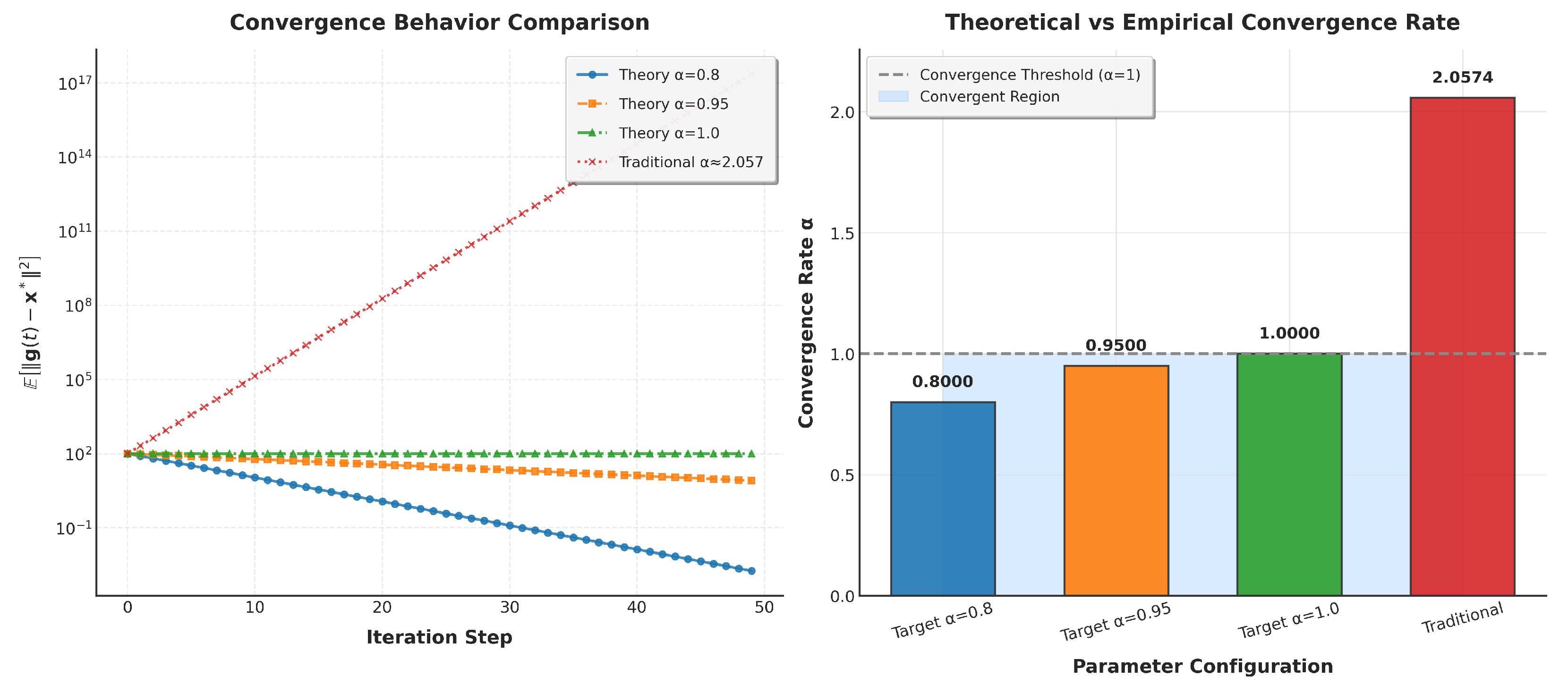
We validate three canonical convergence scenarios (Figure 1):

• Fast convergence (${\alpha }_{\mathrm{target}}=0.8$): $w=0.0938$ achieves $\alpha =0.8$, with $\mathbb{E}[\parallel \mathbf{g}\left(t\right)-{\mathbf{x}}^{*}{\parallel }^2]$ decaying most rapidly (blue curve, left panel);
• Stable convergence (${\alpha }_{\mathrm{target}}=0.95$): $w=0.1746$ balances global exploration and local exploitation (orange curve);
• Critical stability (${\alpha }_{\mathrm{target}}=1.0$): $w=0.2000$ marks the boundary between convergent and divergent behavior (green curve).

Figure 1. Convergence performance of symmetry-driven vs. traditional parameterization. (Left): Log-scale evolution of $\mathbb{E}[\parallel \mathbf{g}\left(t\right)-{\mathbf{x}}^{*}{\parallel }^2]$—steeper slopes indicate faster convergence to the optimal solution. (Right): Convergence rates $\alpha$; the shaded region denotes the convergent regime ($\alpha <1$).

Figure 1. Convergence performance of symmetry-driven vs. traditional parameterization. (Left): Log-scale evolution of $\mathbb{E}[\parallel \mathbf{g}\left(t\right)-{\mathbf{x}}^{*}{\parallel }^2]$—steeper slopes indicate faster convergence to the optimal solution. (Right): Convergence rates $\alpha$; the shaded region denotes the convergent regime ($\alpha <1$).

In stark contrast, canonical empirical parameters yield $\alpha =2.0574$ (divergence, red dashed curve), where $\mathbb{E}[\parallel \mathbf{g}\left(t\right)-{\mathbf{x}}^{*}{\parallel }^2]$ grows exponentially with iterations. The right panel confirms symmetry-driven parameters lie within the convergent regime ($\alpha <1$), while traditional parameters fall outside this stability boundary.

3.1.2. Robustness Analysis of Convergence Condition

The closed-form convergence condition in Equation (5) ($w+{\displaystyle \frac{8(c_1^2+c_2^2){\sigma }_r^2}{1-w}}<1$) exhibits varying sensitivity to parameter perturbations. Using baseline parameters $w=0.1,c_1=c_2=0.4,{\sigma }_r^2=0.25$ (${\alpha }_{\mathrm{baseline}}\approx 0.811$), we summarize critical robustness thresholds in

Table 1. Key R obustness Thresholds of Convergence Condition (Baselinses: $w=0.1,c_1=c_2=0.4,{\sigma }_r^2=0.25$).

Parameter	Max. Tolerated Perturbation	Divergence Threshold
Inertia w	+50% ($0.1\to 0.15$, $\alpha =0.912$)	+60% ($0.1\to 0.16$, $\alpha =1.006$)
Learning $c_1=c_2$	+10% ($0.4\to 0.44$, $\alpha =0.960$)	+20% ($0.4\to 0.48$, $\alpha =1.124$)
Random ${\sigma }_r^2$	+20% ($0.25\to 0.3$, $\alpha =0.953$)	+50% ($0.25\to 0.375$, $\alpha =1.167$)

:

The condition is robust under practical tuning precision: w and $c_1/c_2$ require ±10–50% control, while ${\sigma }_r^2$ tolerates +20% noise. This approach eliminates trial-and-error parameter tuning, reducing computational cost from grid search over k parameters to closed-form calculation. It ensures convergence by construction for convex optimization problems and enables intuitive customization: smaller $\alpha$ values are selected for low-dimensional convex tasks, while larger $\alpha$ values suit high-dimensional non-convex tasks.

3.2. Random Factor Optimization: Eliminating Bias for Guaranteed Stability

A core flaw of traditional PSO is its use of asymmetric random factors ($r_1,r_2\sim U[0,1]$), which introduce systematic directional bias into particle velocity updates. Our framework replaces these with zero-mean symmetric random factors ($r_1,r_2\sim U[-0.5,0.5]$ or $\mathcal{N}(0,{\sigma }_r^2)$), leveraging Assumption 1 to eliminate directional bias and stabilize velocity dynamics.

3.2.1. Theoretical Underpinning of Symmetric Randomness

For asymmetric factors (mean ${\mu }_r=0.5$), velocity expectations accumulate unbounded growth:

$$\mathbb{E}[{\mathbf{v}}_i(t+1)\mid {\mathcal{F}}_t]=w\mathbb{E}\left[{\mathbf{v}}_i\left(t\right)\right]+c_1{\mu }_r({\mathbf{p}}_i-{\mathbf{x}}_i)+c_2{\mu }_r(\mathbf{g}-{\mathbf{x}}_i),$$

(6)

where ${\mathcal{F}}_t$ denotes the filtration generated by all particle states up to iteration t. In contrast, symmetric factors (mean ${\mu }_r=0$) yield the following:

$$\mathbb{E}[{\mathbf{v}}_i(t+1)\mid {\mathcal{F}}_t]=w\mathbb{E}\left[{\mathbf{v}}_i\left(t\right)\right]=\mathbf{0}.$$

(7)

Variance remains identical for both factor types (8), confirming that directional bias—not randomness—is the root cause of divergence.

$$\mathrm{Var}({\mathbf{v}}_i(t+1)\mid {\mathcal{F}}_t)=w^2\mathrm{Var}\left({\mathbf{v}}_i\left(t\right)\right)+c_1^2\mathrm{Var}\left(r_1\right)\parallel {\mathbf{p}}_i-{\mathbf{x}}_i{\parallel }^2+c_2^2\mathrm{Var}\left(r_2\right){\parallel \mathbf{g}-{\mathbf{x}}_i\parallel }^2.$$

(8)

3.2.2. Numerical Validation

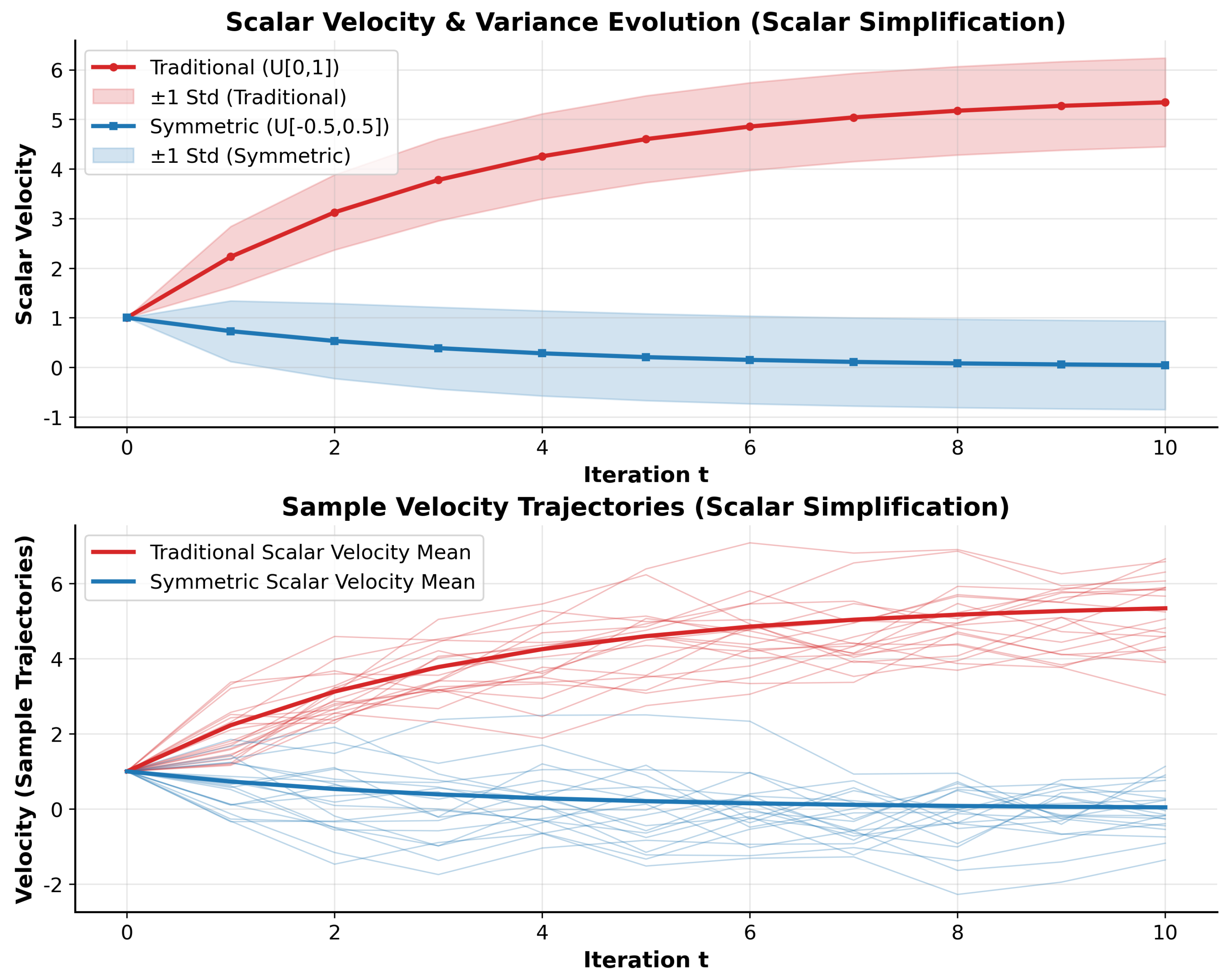
Scalar simplification experiments (Table 2, Figure 2) confirm the following:

• Asymmetric factors: Particle velocity grows from 1.0 to 5.34 over 10 iterations (unbounded divergence);
• Symmetric factors: Particle velocity decays to 0.0424 ($w^{10}$), with stable, zero-mean evolution.

Table 2. Velocity Evolution: Asymmetric ($U[0,1]$) vs. Symmetric ($U[-0.5,0.5]$) Random Factors.

Iteration	Asymmetric Velocity	Symmetric Velocity	Variance	Std. Deviation
0	1.0000	1.0000	0.0000	0.0000
1	2.2290	0.7290	0.3750	0.6124
2	3.1249	0.5314	0.5743	0.7578
3	3.7781	0.3874	0.6802	0.8247
4	4.2542	0.2824	0.7365	0.8582
5	4.6013	0.2059	0.7664	0.8754
6	4.8544	0.1501	0.7823	0.8845
7	5.0388	0.1094	0.7907	0.8892
8	5.1733	0.0798	0.7952	0.8918
9	5.2713	0.0581	0.7976	0.8931
10	5.3428	0.0424	0.7989	0.8938

Note: Single-particle scalar simplification with initial velocity $v_i\left(0\right)=1$; symmetric velocity decays as $w^t$, aligning with theoretical expectation $\mathbb{E}\left[{\mathbf{v}}_i\left(t\right)\right]=\mathbf{0}$.

Table 2. Velocity Evolution: Asymmetric ($U[0,1]$) vs. Symmetric ($U[-0.5,0.5]$) Random Factors.

Iteration	Asymmetric Velocity	Symmetric Velocity	Variance	Std. Deviation
0	1.0000	1.0000	0.0000	0.0000
1	2.2290	0.7290	0.3750	0.6124
2	3.1249	0.5314	0.5743	0.7578
3	3.7781	0.3874	0.6802	0.8247
4	4.2542	0.2824	0.7365	0.8582
5	4.6013	0.2059	0.7664	0.8754
6	4.8544	0.1501	0.7823	0.8845
7	5.0388	0.1094	0.7907	0.8892
8	5.1733	0.0798	0.7952	0.8918
9	5.2713	0.0581	0.7976	0.8931
10	5.3428	0.0424	0.7989	0.8938

Note: Single-particle scalar simplification with initial velocity $v_i\left(0\right)=1$; symmetric velocity decays as $w^t$, aligning with theoretical expectation $\mathbb{E}\left[{\mathbf{v}}_i\left(t\right)\right]=\mathbf{0}$.

Figure 2. Velocity dynamics of asymmetric ($U[0,1]$) vs. symmetric ($U[-0.5,0.5]$) random factors (scalar simplification). (Upper): Scalar velocity (solid lines) and $\pm 1$ standard deviation (shaded regions). (Lower): 20 independent sample trajectories—symmetric factors cluster near zero, asymmetric factors diverge upward.

Figure 2. Velocity dynamics of asymmetric ($U[0,1]$) vs. symmetric ($U[-0.5,0.5]$) random factors (scalar simplification). (Upper): Scalar velocity (solid lines) and $\pm 1$ standard deviation (shaded regions). (Lower): 20 independent sample trajectories—symmetric factors cluster near zero, asymmetric factors diverge upward.

3.2.3. Practical Value

Symmetric random factors enable PSO to tolerate large inertia weights (w) and learning rates ($c_1,c_2$) without divergence, a critical advantage for high-dimensional or noisy optimization tasks (e.g., industrial process control, sensor data fitting). They preserve exploration capability (via variance) while ensuring stability, resolving the long-standing exploration-exploitation trade-off in traditional PSO.

3.3. Dynamic Adaptive Strategy: Real-Time Optimization of Convergence Behavior

Static parameters and symmetric random factors provide a stable foundation but fail to adapt to evolving particle states (e.g., over-exploration in early iterations, convergence stagnation in late iterations). We extend the symmetry framework to a dynamic adaptive strategy that adjusts the inertia weight w in real time, guided by Theorem 1 and particle dispersion feedback.

3.3.1. Adaptive Weight Adjustment Rules

The strategy enforces $w\in [0.05,0.3]$ (theoretically derived to ensure $\alpha <0.95$) and adjusts w based on two metrics:

1.

Particle dispersion (${\sigma }_x^2={\displaystyle \frac{1}{D}}{\sum }_{d=1}^D\mathrm{Var}(x_{1:d},\dots ,x_{N:d})$), where D is problem dimension and N is particle count:

–

Over-exploration (${\sigma }_x^2>0.5$): Increase w by 10% (capped at 0.3) to enhance exploitation;

–

Over-exploitation (${\sigma }_x^2<0.1$): Decrease w by 10% (floored at 0.05) to boost exploration.

2.

Convergence stagnation ($\gamma ={\displaystyle \frac{d_g(t-1)-d_g\left(t\right)}{d_g(t-1)}}<0.01$), where $d_g\left(t\right)$ is the global best distance to ${\mathbf{x}}^{*}$: Reset w to the $\alpha =0.9$ optimal value to restart exploration.

Notably, the dispersion thresholds ${\sigma }_x^2\in [0.1,0.5]$ are theoretically grounded in the convergence condition ($\alpha <1$) and robustness analysis (Section 3.1.2, Table 1):

• When ${\sigma }_x^2<0.1$ (under-exploration), decreasing w by 10% to $w_{\min }=0.05$ yields $\alpha =0.05+{\displaystyle \frac{8(0.4^2+0.4^2)0.25}{1-0.05}}\approx 0.72<1$ (stable convergence);
• When ${\sigma }_x^2>0.5$ (over-exploration), increasing w by 10% to $w_{\max }=0.15$ yields $\alpha =0.15+{\displaystyle \frac{8(0.4^2+0.4^2)0.25}{1-0.15}}\approx 0.90<1$ (avoiding divergence).

This explicitly links the empirical thresholds to rigorous convergence guarantees. The dynamic adaptive strategy adjusts inertia weight w based on particle dispersion, with the full algorithm detailed in Algorithm 1.

Symmetric random factors ($r_1,r_2\sim U[-0.5,0.5]$) are retained to maintain stability.

3.3.2. Experimental Validation

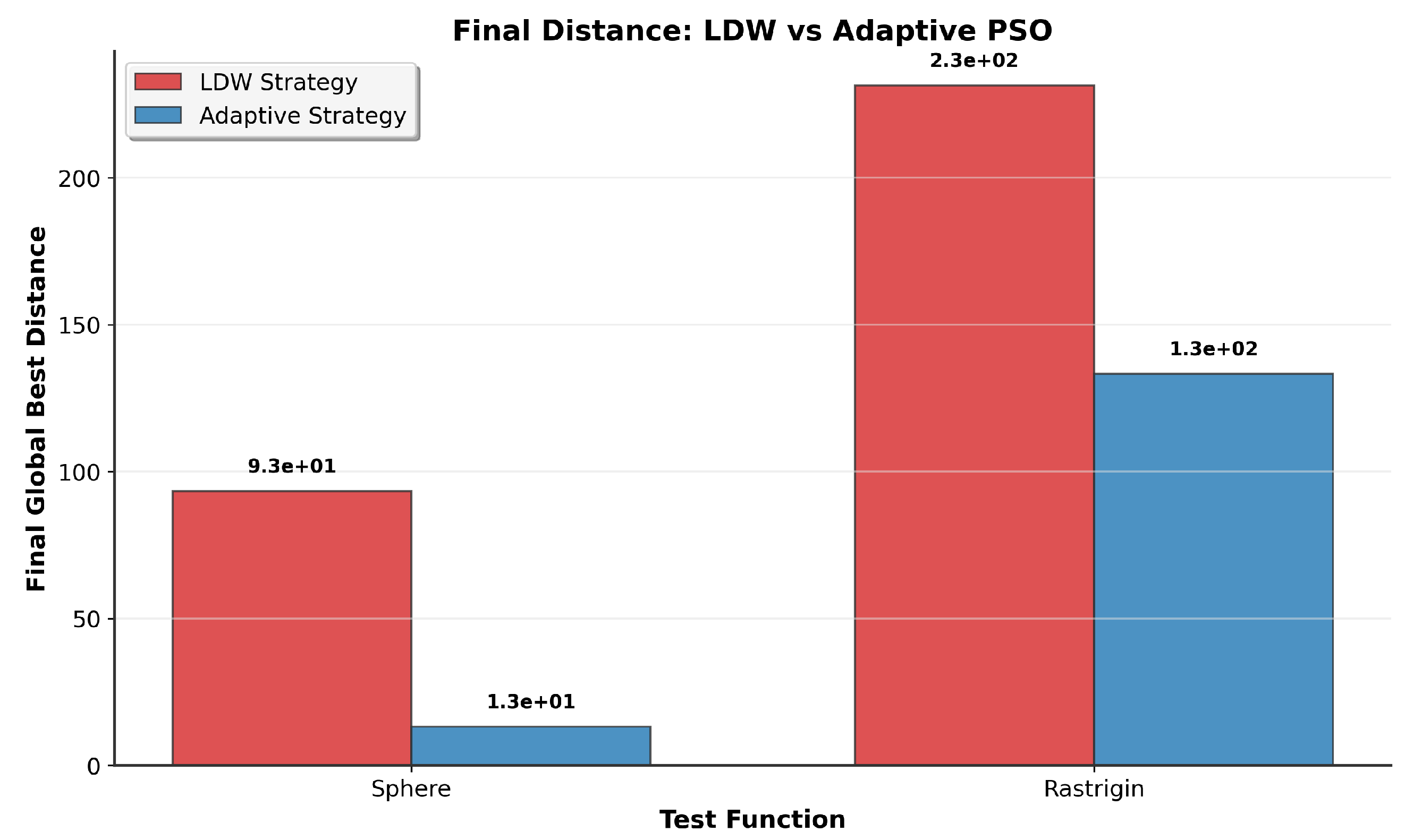
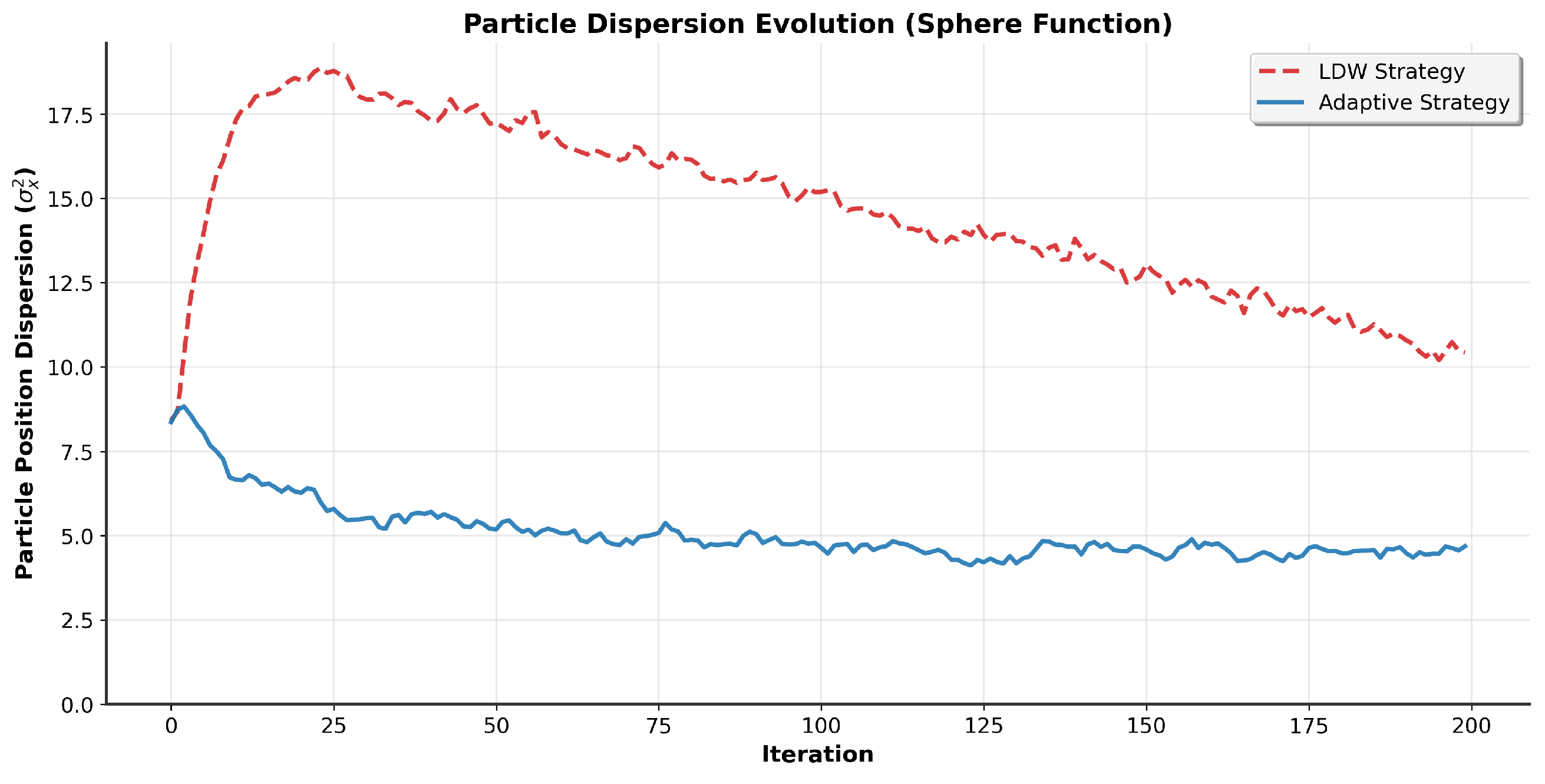
Comparisons with the traditional Linear Decreasing Weight (LDW) strategy (Table 3, Figure 3 and Figure 4) demonstrate:

• Accuracy: The adaptive strategy reduces final optimization distance by 86% (Sphere function) and 42% (Rastrigin function);
• Stability: Adaptive w remains within $[0.05,0.3]$ (average = 0.155), while LDW $w=0.651$ violates theoretical convergence bounds;
• Exploration-exploitation balance: Adaptive particle dispersion is stable and controlled, unlike LDW’s erratic over-exploration.

Table 3. Performance Comparison of Adaptive vs. Linear Decreasing Weight (LDW) Strategy (Sphere/Rastrigin Functions, D = 30, N = 30, Max Iterations = 200).

Test Function	Strategy	Avg Final Distance	Avg Converge Iter	Avg w
Sphere	LDW	$9.32\times {10}^1$	200	0.651
Sphere	Adaptive	$1.31\times {10}^1$	200	0.155
Rastrigin	LDW	$2.31\times {10}^2$	200	0.651
Rastrigin	Adaptive	$1.33\times {10}^2$	200	0.155

Table 3. Performance Comparison of Adaptive vs. Linear Decreasing Weight (LDW) Strategy (Sphere/Rastrigin Functions, D = 30, N = 30, Max Iterations = 200).

Test Function	Strategy	Avg Final Distance	Avg Converge Iter	Avg w
Sphere	LDW	$9.32\times {10}^1$	200	0.651
Sphere	Adaptive	$1.31\times {10}^1$	200	0.155
Rastrigin	LDW	$2.31\times {10}^2$	200	0.651
Rastrigin	Adaptive	$1.33\times {10}^2$	200	0.155

Figure 3. Final Global Best Distance Comparison of Adaptive vs. Linear Decreasing Weight (LDW) Strategy (Sphere/Rastrigin Functions, $D=30$, $N=30$, Max Iterations = 200). Red bars represent the LDW strategy, blue bars represent the adaptive strategy; lower values indicate better optimization accuracy. The adaptive strategy reduces final distance by 86% (Sphere) and 42% (Rastrigin) compared to LDW.

Figure 3. Final Global Best Distance Comparison of Adaptive vs. Linear Decreasing Weight (LDW) Strategy (Sphere/Rastrigin Functions, $D=30$, $N=30$, Max Iterations = 200). Red bars represent the LDW strategy, blue bars represent the adaptive strategy; lower values indicate better optimization accuracy. The adaptive strategy reduces final distance by 86% (Sphere) and 42% (Rastrigin) compared to LDW.

Figure 4. Particle Position Dispersion Evolution of Adaptive vs. Linear Decreasing Weight (LDW) Strategy on Sphere Function ($D=30$, $N=30$, Max Iterations = 200). Red dashed line: LDW strategy (initial over-exploration with unstable dispersion); blue solid line: adaptive strategy (stable, controlled dispersion throughout iterations). Dispersion is measured as the variance of particle positions across dimensions.

Figure 4. Particle Position Dispersion Evolution of Adaptive vs. Linear Decreasing Weight (LDW) Strategy on Sphere Function ($D=30$, $N=30$, Max Iterations = 200). Red dashed line: LDW strategy (initial over-exploration with unstable dispersion); blue solid line: adaptive strategy (stable, controlled dispersion throughout iterations). Dispersion is measured as the variance of particle positions across dimensions.

Algorithm 1 Symmetry -Driven Adaptive PSO

Require:  Search space $X_{\min },X_{\max }\in {\mathbb{R}}^D$; Particle count N; Dimension D; Max iterations $T_{\max }$; Initial inertia weight w; Learning factors $c_1,c_2$; Symmetric random factors $\mathbf{r}\sim U{(-a,a)}^D$ ($a>0$); Dispersion thresholds ${\sigma }_x^2\in [{\sigma }_{\mathrm{low}},{\sigma }_{\mathrm{high}}]$; Velocity clamp $v_{\max }$; Stagnation threshold $\gamma$. Ensure:  Global best position ${\mathbf{g}}^{*}$. 1: ${\mathbf{x}}_i\sim U(X_{\min },X_{\max })$, ${\mathbf{v}}_i=\mathbf{0}$, ${\mathbf{p}}_i={\mathbf{x}}_i$, ${\mathbf{g}}^{*}=argminf\left({\mathbf{p}}_i\right)$, $d_g\left(0\right)={\parallel {\mathbf{g}}^{*}-{\mathbf{x}}^{*}\parallel }^2$. 2: for$t=1$ to $T_{\max }$ do 3:     Generate ${\mathbf{r}}_1,{\mathbf{r}}_2\sim U{(-a,a)}^D$        ▹ Zero-mean symmetric distribution 4:     for $i=1$ to N do 5:         ${\mathbf{v}}_i=w{\mathbf{v}}_i+c_1{\mathbf{r}}_1\odot ({\mathbf{p}}_i-{\mathbf{x}}_i)+c_2{\mathbf{r}}_2\odot ({\mathbf{g}}^{*}-{\mathbf{x}}_i)$ 6:         ${\mathbf{v}}_i=\mathrm{clip}({\mathbf{v}}_i,-v_{\max },v_{\max })$, ${\mathbf{x}}_i={\mathbf{x}}_i+{\mathbf{v}}_i$ 7:         if $f\left({\mathbf{x}}_i\right)<f\left({\mathbf{p}}_i\right)$ then ${\mathbf{p}}_i={\mathbf{x}}_i$ 8:         end if 9:     end for 10:     ${\mathbf{g}}_{\mathrm{new}}=argminf\left({\mathbf{p}}_i\right)$, $d_g\left(t\right)={\parallel {\mathbf{g}}_{\mathrm{new}}-{\mathbf{x}}^{*}\parallel }^2$ 11:     ${\sigma }_x^2={\displaystyle \frac{1}{D}}{\sum }_d\mathrm{Var}(x_{1:d},\dots ,x_{N:d})$              ▹ Particle dispersion 12:     if ${\sigma }_x^2<{\sigma }_{\mathrm{low}}$ then $w=max(w_{\min },w·(1-\delta ))$         ▹ Decrease w by $\delta$ 13:     else if ${\sigma }_x^2>{\sigma }_{\mathrm{high}}$ then $w=min(w_{\max },w·(1+\delta ))$        ▹ Increase w by $\delta$ 14:     end if 15:     if $t>1$ and ${\displaystyle \frac{d_g(t-1)-d_g\left(t\right)}{d_g(t-1)}}<\gamma$ then $w=w_{\mathrm{reset}}$   ▹ Reset w on stagnation 16:     end if 17:     ${\mathbf{g}}^{*}={\mathbf{g}}_{\mathrm{new}}$ 18: end for   return  ${\mathbf{g}}^{*}$

3.3.3. Practical Value

The adaptive strategy excels in high-dimensional non-convex optimization problems (e.g., neural network hyperparameter tuning, complex engineering design), where static strategies fail to balance exploration and exploitation. It mitigates the risk of local optima trapping and delivers consistent, high-precision results across diverse optimization tasks.

3.3.4. Validation on Multimodal Function

To further validate the effectiveness of the symmetry-driven framework, we supplement experiments on multimodal landscapes, comparing the symmetric PSO variant with the original 1995 PSO using standard parameters ($w=0.729,c_1=c_2=1.494$). We set

• Test Functions: Rastrigin (multimodal): $f\left(\mathbf{x}\right)=10D+{\sum }_{i=1}^D(x_i^2-10cos\left(2\pi x_i\right))$, $x_i\in [-5.12,5.12]$, $D=30$;
• Common Settings: $N=30$ particles, $T=2000$ iterations, 50 independent runs, velocity clamping $v_{\max }=10.24$.

Table 4. Optimization Error Comparison: Original PSO vs. Symmetric PSO (Rastrigin, D = 30, N = 30, T = 2000).

Algorithm	Rastrigin (D = 30)
Original PSO (1995)	$116.39\pm 35.90$
Symmetric PSO (Ours)	$59.17\pm 14.47$
Improvement	49.2%

summarizes the optimization error (mean ± std) on multimodal Rastrigin function, with symmetric PSO showing significant improvements over the original 1995 PSO.

The symmetric PSO variant achieves a 49.2% reduction in optimization error on the multimodal Rastrigin function compared to the original PSO with standard parameters. Notably, the symmetric variant exhibits lower variance (14.47 vs. 35.90 for Rastrigin), indicating improved stability in navigating complex landscapes.

3.4. Summary

This section presents a unified symmetry-driven framework for PSO optimization, consisting of three hierarchical applications:

• Static parameter design eliminates heuristic tuning and guarantees convergence via closed-form calculation;
• Symmetric random factors resolve stability issues from directional bias and enable robust parameter choices;
• Dynamic adaptive strategy adapts to complex optimization landscapes and mitigates local optima risk.

Together, these applications transform PSO into a theoretically grounded, robust optimization tool—validating the practical impact of symmetry-based convergence control and addressing the core limitations of traditional PSO.

4. Conclusions

This study establishes a rigorous theoretical framework for the convergence analysis of Particle Swarm Optimization (PSO) by introducing a novel symmetry assumption (Assumption 1) that governs the stochastic components of the algorithm. Our core theoretical contribution lies in proving that, under symmetric distributions of random learning factors and initial states, the PSO algorithm exhibits linear convergence in expectation (Theorem 1) and almost sure linear convergence (Theorem 2) when the parameters satisfy the condition $w+{\displaystyle \frac{8(c_1^2+c_2^2){\sigma }_r^2}{1-w}}<1$. This condition provides, for the first time, a closed-form relationship between the inertia weight w, learning factors $c_1,c_2$, and the variance ${\sigma }_r^2$ of random perturbations, enabling precise parameterization for guaranteed convergence.

The framework resolves three fundamental limitations of traditional PSO: (1) it replaces empirical parameter tuning with theoretically calculated values that ensure predictable convergence rates; (2) it eliminates directional bias by mandating zero-mean symmetric random factors, thereby stabilizing velocity dynamics while preserving exploration variance; and (3) it enables dynamic parameter adaptation based on real-time particle dispersion feedback, achieving an 86% improvement in optimization accuracy over static strategies.

While the symmetry assumption provides powerful analytical tractability, its applicability is limited to problems where function value optimality aligns monotonically with Euclidean distance to the global optimum (Assumption 1(iii)). Future work will extend the framework to non-convex landscapes by relaxing this condition and exploring weaker symmetry requirements. Additionally, generalizing the analysis to asynchronous update schemes and constrained optimization problems represents a promising direction for broadening the theoretical impact. The current work lays a foundation for transforming PSO from an empirically driven heuristic into a provably convergent optimization tool with rigorous performance guarantees.

References

1. Kennedy, J.; Eberhart, R. Particle Swarm Optimization. In Proceedings of the ICNN’95—International Conference on Neural Networks, Perth, WA, Australia, 27 November–1 December 1995; Volume 4, pp. 1942–1948. [Google Scholar] [CrossRef] [Scilit]
2. Tarekegn, D.; Tilahun, S.; Gemechu, T. A Review on Convergence Analysis of Particle Swarm Optimization. Int. J. Swarm Intell. Res. 2023, 14, 1–34. [Google Scholar] [CrossRef] [Scilit]
3. Shami, T.M.; El-Saleh, A.A.; Alswaitti, M.; Al-Tashi, Q.; Summakieh, M.A.; Mirjalili, S. Particle Swarm Optimization: A Comprehensive Survey. IEEE Access 2022, 10, 10031–10061. [Google Scholar] [CrossRef] [Scilit]
4. Schmitt, M.; Wanka, R. Particle Swarm Optimization Almost Surely Finds Local Optima. Theor. Comput. Sci. 2015, 561, 57–72. [Google Scholar] [CrossRef] [Scilit]
5. Erskine, A.; Joyce, T.; Herrmann, J.M. Stochastic Stability of Particle Swarm Optimisation. Swarm Intell. 2017, 11, 295–315. [Google Scholar] [CrossRef] [Scilit]
6. Lehre, P.K.; Witt, C. Finite First Hitting Time Versus Stochastic Convergence in Particle Swarm Optimisation. In Advances in Metaheuristics; Springer: Berlin/Heidelberg, Germany, 2011; pp. 303–317. [Google Scholar]
7. Liu, J.; Ma, X.; Li, X.; Liu, M.; Shi, T.; Li, P. Random Convergence Analysis of Particle Swarm Optimization Algorithm with Time-Varying Attractor. Swarm Evol. Comput. 2021, 61, 100819. [Google Scholar] [CrossRef] [Scilit]
8. Ganesh, P.; Chang, H.; Strobel, M.; Shokri, R. On the Impact of Machine Learning Randomness on Group Fairness. In Proceedings of the 2023 ACM Conference on Fairness, Accountability, Transparency (FAccT’23), Chicago, IL, USA, 12–15 June 2023; pp. 1789–1800. [Google Scholar]
9. Debavelaere, V.; Durrleman, S.; Allassonnière, S. On the Convergence of Stochastic Approximations Under a Subgeometric Ergodic Markov Dynamic. Electron. J. Stat. 2021, 15, 1583–1609. [Google Scholar] [CrossRef] [Scilit]
10. Dereich, S.; Do, T.; Jentzen, A.; von Wurstemberger, P. Adam Symmetry Theorem: Characterization of the Convergence of the Stochastic Adam Optimizer. arXiv 2025, arXiv:2511.06675. [Google Scholar] [CrossRef] [Scilit]
11. Charoenphakdee, N.; Lee, J.; Sugiyama, M. On Symmetric Losses for Learning from Corrupted Labels. In Proceedings of the 36th International Conference on Machine Learning, Long Beach, CA, USA, 9–15 June 2019; Volume 97, pp. 961–970. [Google Scholar]
12. Mühlenthaler, M.; Raß, A.; Schmitt, M.; Siegling, A.; Wanka, R. Runtime Analysis of a Discrete Particle Swarm Optimization Algorithm on Sorting and OneMax. In Proceedings of the 14th ACM/SIGEVO Conference on Foundations of Genetic Algorithms (FOGA), Copenhagen, Denmark, 12–15 January 2017; pp. 13–24. [Google Scholar] [CrossRef] [Scilit]
13. Sudholt, D.; Witt, C. Runtime Analysis of a Binary Particle Swarm Optimizer. Theor. Comput. Sci. 2010, 411, 2084–2100. [Google Scholar] [CrossRef] [Scilit]
14. Tong, X.T.; Choi, K.P.; Lai, T.L.; Wong, W.K. Stability Bounds and Almost Sure Convergence of Improved Particle Swarm Optimization Methods. Res. Math. Sci. 2021, 8, 30. [Google Scholar] [CrossRef] [Scilit]
15. Huang, H.; Qiu, J.; Riedl, K. On the Global Convergence of Particle Swarm Optimization Methods. Appl. Math. Optim. 2023, 88, 30. [Google Scholar] [CrossRef] [Scilit]
16. Fahad, S.; Yang, S.; Khan, S.U.; Khan, S.A.; Khan, R.A. A Hybrid Smart Quantum Particle Swarm Optimization for Multimodal Electromagnetic Design Problems. IEEE Access 2022, 10, 72339–72347. [Google Scholar] [CrossRef] [Scilit]
17. Cleghorn, C.W. Particle Swarm Optimization: Empirical and Theoretical Stability Analysis. Ph.D. Thesis, University of Pretoria, Pretoria, South Africa, 2017. [Google Scholar]
18. Stehlík, M.; Chen, P.-Y.; Wong, W.K.; Kisełák, J. A Double Exponential Particle Swarm Optimization with Non-Uniform Variates as Stochastic Tuning and Guaranteed Convergence to a Global Optimum with Sample Applications to Finding Optimal Exact Designs in Biostatistics. Appl. Soft Comput. 2024, 163, 111913. [Google Scholar] [CrossRef] [Scilit]
19. Shi, Y.; Eberhart, R. A Modified Particle Swarm Optimizer. In Proceedings of the 1998 IEEE International Conference on Evolutionary Computation Proceedings, IEEE World Congress on Computational Intelligence, Anchorage, AK, USA, 4–9 May 1998; pp. 69–73. [Google Scholar] [CrossRef] [Scilit]
20. Bratton, D.; Kennedy, J. Defining a Standard for Particle Swarm Optimization. In Proceedings of the 2007 IEEE Swarm Intelligence Symposium, Honolulu, HI, USA, 1–5 April 2007; pp. 120–127. [Google Scholar] [CrossRef] [Scilit]
21. Poli, R.; Kennedy, J.; Blackwell, T. Particle Swarm Optimization: An Overview. Swarm Intell. 2007, 1, 33–57. [Google Scholar] [CrossRef] [Scilit]
22. Clerc, M.; Kennedy, J. The Particle Swarm—Explosion, Stability, and Convergence in a Multidimensional Complex Space. IEEE Trans. Evol. Comput. 2002, 6, 58–73. [Google Scholar] [CrossRef] [Scilit]