Abstract
Time delays in the images of gravitationally lensed quasars play crucial role in understanding the geometry and physical context of the gravitational lens systems (GLS). In case of the short time delays on hourly/daily timescales, correlating the X-ray/gamma-ray data is the best way to determine them as the variability of quasars at these energies is usually faster than at lower ones. Here, we demonstrate the usage of our web tool for correlation function analysis, applying the cross-correlation (asymmetrical) function to the Chandra and auto-correlation (symmetrical) one to the XMM-Newton light curves of the images of the quasar in the famous GLS Q2237+0305 (“Huchra lens”/“Einstein Cross”). We also describe the way to distinguish between the GLS time delay and periodicity in light curves based on translational symmetry of cross-correlation function in case of periodicity of the signal. We have estimated the delays between the gravitationally lensed images and the timescales of (quasi)periodical flux variations of the quasar in the Einstein Cross.
1. Introduction
Gravitational Lensing (GL) of distant extragalactic sources such as quasars causes the appearance of multiple (two or more) images of the same object [1]. These images have similar spectral properties, but there are delays in time of signal arrival from different images caused by differences in the light paths deflected by the gravitational field of a lens. Measurement of these time delays (and subsequently the time delay cosmological distance) could provide important information about the structure of a gravitational lens system (GLS), and as a part of “Time-delay Cosmography” [2] to make its contribution to the improving accuracy of the determining Hubble constant and other cosmological parameters. The pioneer method for the determination of the Hubble constant was proposed by Refsdal in 1964 [1] and reached its practical development in [3,4], based on 10 GLS. Modern project “Time Delay Cosmography” [2] can include in future several hundreds of them.
Time delays in real extragalactic GLS cover a wide span of values from hours or days to years. The longest time delay of more than six years was found in SDSS J1004+4112 [5]. The shortest time delays on hourly timescales are known in the famous Q2237+0305 “The Einstein Cross” [6]. Recently, GAIA GRAL (GAIA GRAvitational Lens systems) disclosed several GLS with predicted daily time delays according to their lens density model [7].
Correlation analysis is one of the best instruments for determining the time delays in GLS from the light curves of the images of the gravitationally lensed images. For yearly to weekly timescales of delays, optical monitorings such as OGLE (Optical Gravitational Lens Experiment) [8] https://ogle.astrouw.edu.pl/cont/4_main/len/huchra/ (accessed on 24 November 2024) or COSMOGRAIL (COSmological MOnitoring of GRAvItational Lenses) [9] can give the best clue to estimate them with a high level of accuracy. But for the shorter time delays on hourly to daily timescales one need to use X-ray photometry because the variability of quasars at these energies is typically faster. In this work, we demonstrate our web tool for correlation analysis to estimate the time delays in Q2237+0305 “The Einstein Cross” from the Chandra and XMM-Newton photometry data.
In Section 2, we briefly describe the object of our investigation; in Section 3 we perform the reduction of Chandra and XMM-Newton observational data; in Section 4 we introduce some details about the auto/cross-correlation functions and demonstrate our web tool; in Section 5 we perform the correlation analysis and estimate the time delays. Finally, in the last Section 6, we draw our conclusions.
2. Q2237+0305 the Einstein Cross
The GLS Q2237+0305 (Einstein Cross, [10]) consists of a quadruply imaged quasar (with redshift = 1.695) and the nearest known lensing galaxy (with redshift = 0.0395). The time delays between the images in the Einstein Cross are on hourly (less than daily) timescales [6,11]. The timescales of inner optical variations in the quasar are on the level of days; that is why it is unlikely to improve this level of accuracy on the basis of optical light curves [11]. The detection of a variable X-ray flux from this system will lead to better quality of the estimates of the relative time delays between images, both due to faster tempo of X-ray variability and shorter timebins in X-ray observations.
The lens structure models in Q2237+0305 predict the hourly timescale delays, with the longest delays involving the C image. In Table 1 we show the time delay values predicted by various models of the gravitational lens structure.

Table 1.
The model-predicted time delays in Q2237+0305.
Attempts to determine time delays in Q2237+0305 were performed on the basis of long-term optical monitoring [6,11]. The best accuracy of the time delay’s determination was achieved by Berdina and Tsvetkova [11] (AB 4.5 ± 1.9 h, AC 14.2 ± 1.7 h, AD −2.7 ± 4.6 h, BC −19.0 ± 1.6 h, BD −3.0 ± 4.0 h and CD 19.3 ± 2.8 h); however, the uncertainty remains greater than 40% for the shortest delays in the best case (A B).
The first X-ray detection of Q2237+0305 was performed by ROSAT in 1997 [14]; these observations did not show any significant flux variability. After ROSAT, Chandra X-ray Observatory observed this GLS several times in 2000 and 2001 with the Advanced CCD Imaging Spectrometer (ACIS). The longest of these two observations lasting 30 ks carried out in September 2000 had detected the hourly-timescale inner flux variability, which had given a clue to determine the time delay of = hours between two of the four GLS images [15], achieving much better accuracy than that based on the optical monitoring. At the same time, available Chandra observational exposures are not enough to determine time delays between the image C and other images in this system. The first XMM-Newton observation of Q2237+0305 had not revealed any sign of variability on timescales up to 200 s [16]. Later observations of the “Einstein Cross” by Chandra were synchronized in time with the strong microlensing events observed by OGLE. These observations revealed bright microlensing-induced peaks on weekly timescales in the quasar image light curves [17] but did not demonstrate inner quasar variability.
Our analysis includes all available Chandra and XMM-Newton data and enables us to improve the accuracy of the time delay determination, and (for longer-exposure XMM-Newton light curves) to attribute some possible delays found by means of the correlation analysis to that between the image C and other ones.
3. The Data Reduction
In this section, we perform the reduction of the three XMM-Newton observations of the GLS Q2237+0305 taken in 2002, 2016, and 2018 and the whole set of Chandra observations performed during 2000–2019.
3.1. Chandra
The “Einstein Cross” was observed by the Advanced X-ray Astrophysics Facility (AXAF) of the Chandra cosmic mission 40 times total, during the period from 2000 until 2019. These observations are publicly available at the URL: https://heasarc.gsfc.nasa.gov/docs/archive.html (accessed on 1 October 2024).
To process the observational data and reduce them to obtain the images, spectra and light curves of separate quasar images in the Einstein Cross we used the special CIAO 4.17 offline software, which is publicly available at the URL: https://cxc.cfa.harvard.edu/ciao/download/index.html (accessed on 1 October 2024). Primary reduction of the Chandra/AXAF event files was performed using the chandra_repro standard CIAO script. The corresponding source and background counts as well as the background-subtracted light curves of the four images were extracted using the punlearn, dmcopy, pset, and dmextract procedures. The image obtained for the first Chandra observation of the Einstein Cross is shown in the left panel of the Figure 1.
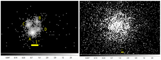
Figure 1.
(Left): Log-scaled Chandra/ACIS image of the Einstein Cross obtained during the first Chandra observation (ID 431, August 2000, units: counts/cm2s), the images A, B, C and D are marked with the corresponding yellow letters, the yellow line shows the 1" angular distance; (right): log-scaled XMM-Newton/EPIC PN image obtained during the last XMM-Newton observation of the Einstein Cross (ID 0823730101, May 2018, units: counts), the yellow line shows the 1" angular distance.
All public Chandra data logs are shown in Table 2. Furthermore, we demonstrate here the relations between the variances on the whole time light curve for each image (here is the mean value of X, is the number of data points in the light curve, and is the mean squared value of X) and the mean squared error .
Table 2.
Chandra/ACIS observations log. The observational data sets included in our analysis are boldfaced.
We involved in our analysis only those of them that have more than 15 ks exposure time or shorter observations one following each other (i.e., one on the next day after another), and with variance of at least two image light curves high enough to enable us to trace out the correlations (i.e., variability is above 10%).
The individual Chandra/ACIS light curves of four images in the Einstein Cross are shown in Figure 2 for two observations, performed in September 2000 and April 2010.
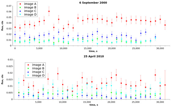
Figure 2.
Chandra/ACIS 1000 s timebin light curves of four images of the Einstein Cross; (upper panel): September 2000, (lower panel): April 2010; abscissa: time in seconds from the observation start, ordinate: flux in counts/s.
3.2. XMM-Newton
Q2237+0305 was observed by the XMM-Newton mission three times. All XMM-Newton observations are publicly available at the HEASARC website at the URL: https://heasarc.gsfc.nasa.gov/docs/archive.html (accessed on 10 October 2023). Table 3 shows log of the XMM-Newton observation data concerning this GLS.
Table 3.
XMM-Newton/EPIC observations log.
The reduction of the datasets was performed with the special SAS software version 22.1.0 (https://www.cosmos.esa.int/web/xmm-newton/sas-installation, accessed on 1 October 2024). The standard SAS chains epproc, emproc, and rgsproc were applied to perform the primary data reduction. The single- and double-photon events were taken into account (i.e., the PATTERN ≤ 4 option was applied). To exclude bad pixels and near-CCD-egde events from our consideration, the filter FLAG = 0 was also applied. The source counts were extracted from the 45 sec-radii circular regions around the source center, and to extract the background counts were chosen the empty regions on the same CCD chip with the same radii. The resulting background–subtracted light curves of all the three EPIC cameras MOS1, MOS2, and PN and spectrometers RGS were merged into one combined 1000 s timebin light curve for each observation. The background-subtracted XMM-Newton light curves of the Einstein Cross are shown in Figure 3. As seen in the last column of Table 3, the variances calculated in the same way as for the Chandra data above in the 1 ks-timebin light curves are high enough to make the correlation analysis effective for them.
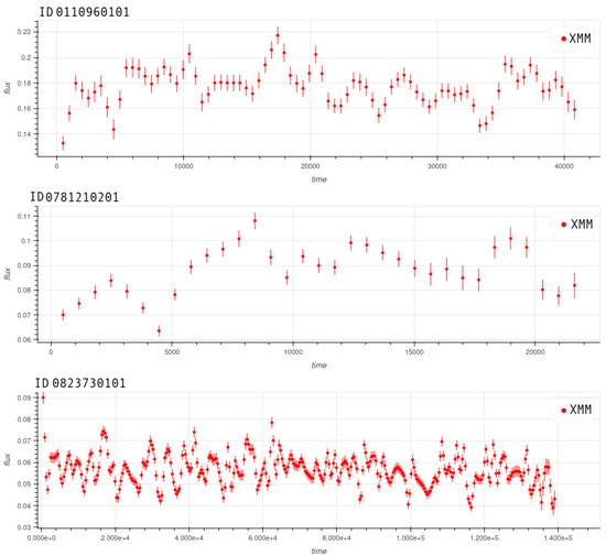
Figure 3.
XMM-Newton total (EPIC+RGS) 1000 s timebin light curves of the Einstein Cross (images are unresolved); (upper panel): observation 0110960101 (2002), (middle panel): observation 0781210201 (2016), (lower panel): observation 0823730101 (2018); abscissa: time in seconds from the observation start, ordinate: total (all four image) flux in counts/s.
4. Auto/Cross-Correlation Functions and the Web Tool for Correlation Analysis
Cross-correlation functions (CCF) are used quite extensively in astronomy to trace the links between variable parameters. For two discrete sets of random observed values X and Y, the cross-correlation function is
where , are the mean values of X and Y in the subset of K values starting from zeroth and the nth ones. and are the variances of Y and X over the subset of Kmax values starting from the nth and zeroth (here and are the mean squared values of Y and X in the subset of Kmax values starting from nth and zeroth ones.
CCF represents the degree of similarity between the two series, one of which can be lagged. The main properties of CCF are as follows:
- Translational symmetry in the case of periodic signals: , where T is the period. The period T is the same for both and . In the case of time lag between nonperiodic signals the symmetry is absent, thus the situation with the lag can be distinguished from that of periodicity using this property of CCF;
- CCF is non commutative if a time lag is present () and it is not symmetric about the abscissa axis;
- If the signals are stochastic, it does not necessarily have a maximum at unless the signals are identical and real.
CCF can be very useful for determining the time delay between two signals, for instance, time delays between images of the same emission source in a GLS. The maximum value of the cross-correlation function indicates the value of the time delay when the signals are best aligned; thus the time delay between the two signals is determined by the argument of the maximum of the cross-correlation, namely:
The autocorrelation function (ACF) is similar to CCF but uses the same series twice instead of the two different ones (one beginning from its origin and the other lagged with varying value of the lag). This makes an ACF commutative and symmetrical about the abscissa axis anyway; additionally, it always has the maximum at = 0.
As well as CCF, ACF can be the tool to reveal periodicity in the signal (in such a case, ACF would also be periodic) or the superposition of several signals lagged one with respect to another (the case of GL images). Applied to periodic processes, ACF or CCF follows the same pattern as the input signal, reflecting its periodicity. However, we should note that the maximums on the ACF correspond to the input’s periodicity rather than the time delays; in the case of CCF for Chandra light curves one should take this into account as well, as the maximums on CCF will be shifted by the values of , where T is a period and n is an integer number (order of maximum). This causes an ambiguity in terms of T in the determination of . Thus, to estimate the time delay between the two images, it is not enough to subtract the value of the period, as one needs to presume the range of possible value of the time delay based on the other observations.
To make the correlation analysis more available for astronomical purposes and beyond them we have created the web tool (which is now under development at https://www.ict.inaf.it/gitlab/olena.fedorova/autocorrelationfunctions, accessed on 15 October 2023) with the possibility to choose the type of analysis (cross-correlation or autocorrelation), upload files for analysis, re-bin and regularize the data in case of necessity, plot the signals and CCF/ACF and generate the CCF/ACF error bars using the Montecarlo technique.
In the next section, we apply this technique to Chandra and XMM-Newton light curves.
5. Time Delays in Q2237+0305 Images
The angular resolution of Chandra ensures the separation of the images of quasar in this GLS. This makes us sure that the delays we can determine from the CCF are really those between the two images whose light curves we analyze. However, the longest exposures provided by Chandra are on the level of 30 ks and thus we cannot see the longer time delays from Chandra light curves and corresponding CCF. This makes them useless for C image in Q2237+0305 in the sense of time delay determination.
XMM-Newton, on the one hand, have significantly longer exposures (upto 150 ks), and longer time delays can be seen as well. However, on the other hand, its angular resolution is much worse than that of Chandra, and the images cannot be resolved with it, giving us only one total light curve for all images. That is why we cannot be sure when attributing the time delays found in XMM-Newton all-images light curve.
5.1. Chandra
From our consideration we excluded the Chandra observations with exposures shorter than 15 ks and those with variances in all images in 1000 s-bin light curves was lower than 1.0. The observations in which time delays or periodicity were detected are shown in Table 4. Some CCF are shown in Figure 4. The only two 15 ks exposure observations considered here are 13,191 and 13,195, performed one a day after another with a time lag of close to 40 h. There are signs of periodicity during both observations, but we have not disclosed here the correlation peaks between the light curves of C and A or B images, which could be interpreted as the consequences of GL-induced time delay.
Table 4.
Chandra/ACIS time delays between images and periodicity (in hours) based on the cross-correlation analysis. In case of periodicity we had chosen among the correlational maximums those closest to the values of time delays obtained for the observational periods with no periodicity. These are boldfaced as well as the time delays for cases with no periodicity.
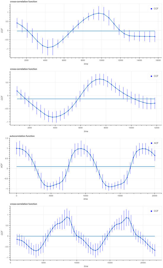
Figure 4.
Chandra/ACIS CCF corresponding to the observations: ID 431, August 2000, images D and A, images A and B, ACF of image D during the observation ID 12832 (December 2012), CCF for the same observation between images C and D; abscissa: time in seconds.
During some of the observational periods, the light curves of images were demonstrating periodicity. In this case, as we had mentioned above in Section 4, we had chosen among the two or three correlational maximums those that are closest to the values of the time delays obtained for the observational periods with no signs of signal periodicity. These are boldfaced in Table 4 and taken into account when calculating the mean values of the time delays. The averaged values of the time delay between images A and B are compatible within the error bars with those found by Dai et al. , [15], Berdina et al. (4.5 ± 1.9, [11]) as well as with the values predicted by Bar Accounted [12] SIE and NSIE + models [13]. The time delays between images D and A (with D leading), D and B are also compatible with those found in Berdina [11] (2.7 ± 4.6, 3.0 ± 4.0), but both are lower than the values predicted by SIE and NSIE + models [13] and closer to the values predicted by Bar Accounted model [12]. At the same time, we should note that the time delays can vary due to the effect of gravitational mesolensing by stellar clusters or dark matter substructures [18,19,20,21].
As we had mentioned above, all the model predicted time delays between image C and other images are longer than 15 h [12,13], and thus even the longest Chandra exposures are not enough to detect them. We have performed here the cross-correlation analysis of image C versus other images and found no appearances of correlational time delays, which can be considered as a sign that they are longer than the time exposures, i.e., 8 h in our case. At the same time CCF analysis of the two subsequent short exposure observations performed in 2010 with near 40 h lag between revealed two peaks at 43 ± 0.3 (C B) and 43.9 ± 0.3 (C A). Taking into account the periodicity of the signals during both these observations and the fact that the model-predicted values are significantly shorter, the interpretation of the nature of these peaks as time delay-induced looks doubtful.
5.2. XMM-Newton
Three observations of XMM-Newton demonstrate enough variability in 1000 s-bin light curves, so we performed the ACF analysis for all of them, despite the fact that the exposure of the second one is quite short (25 ks). These ACF are shown in Figure 5; the maximums found on the ACF and their interpretations are shown in Table 5.
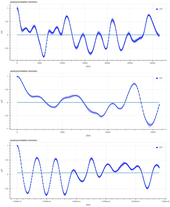
Figure 5.
XMM-Newton ACF corresponding to combined light curves obtained during all the observations; (upper panel): observation 0110960101 (2002), (middle panel): observation 0781210201 (2016), (lower panel): observation 0823730101 (2018); abscissa: time in seconds, ordinate: ACF.
Table 5.
XMM-Newton time delays (in hours) between images based on the autocorrelation analysis.
Time delays of 3.1 ± 0.3 h (first observation) and 2.9 ± 0.3 h (second observation) found in the first two observations can be interpreted rather as the delay between B and A images, as well as the delay of 4.6 ± 0.3 h found in the 2nd observation’s ACF only can be attributed to the delay between D and A images. The time delay of 3.6 ± 0.4 h (third observation) can be attributed to the delays between A and B or D images (or to some combination of them); time delays of 6.0 ± 0.3 h (1st observation) and 6.9 ± 0.6 h (third observation) can be attributed to the delay between D and B images (Bar Accounted model [12]), as well as 8.1 ± 0.3 h found during the 1st one (SIE and NSIE + lens models for this GLS [13]). Longer time delays are found in the third and longest XMM-Newton light curve are h, 25.0 ± 1.7 h, and 29.7 ± 0.8 h. The first of them agrees with the value found for images C (leading) and A or B in [11]; the interpretation of the other two is unclear.
5.3. Periodicity
The phenomenon of quasipertiodic oscillations (QPO) with periodicity on a wide span of timescales from seconds to months is supposed to be quite rare in AGNs [22]. However, for seven of the Chandra observations analyzed here the periodicity was detected, thus QPO probable are not rare for this object.
Depending on the value of the oscillation period, QPO can be considered as high-frequency (HF, with the hourly oscillation period) or low frequency (LF, with the period on the timescales from days to months or in rare cases even years). The QPO periods are inversely related to the CMBH mass, i.e., showing shorter periods for lower masses, and longer ones for more massive ones. At the same time, the longest QPO can be associated with binary black hole systems or systems with jet precession.
By means of the correlation analysis we have determined the values of periods of these light curves, shown in Table 3 as well. The shortest of them is 1.2 ± 0.2 h, the longest one is h, thus we observe here the case of HF QPO.
There are many possible physical explanations for the origin of QPO of different frequencies, but it remains controversial. Existing models of QPO suggest that it can be generated by several mechanisms, such as: accretion pulsations and inner accretion disk instabilities, X-ray bright hot blob of matter orbiting the BH, relativistic accretion disk and/or jet oscillations and precession [23,24,25,26,27,28,29], as well as the resonance model [30,31], the acoustic oscillation model [32] and the accretion–ejection instability model [33], and the disco-seismic thin disk oscillations model [34]. The relativistic precession model predicts LF QPO due to internal disk instability and Lense-Thirring precession of jets or internal heat flux or corona [29,35,36]. The accretion flow inhomogeneity orbital motion is rather HF, as well as the resonance model [31]. On the basis of the timescale of oscillation periodicity we can confine the manifold of models appropriate for the concrete case, but not yet to prefer only one of them. In any case, investigating the characteristics of QPO can give us a better understanding of accretion processes and accretion disk structure [22].
One of the models predicting HF QPO, which can explain oscillations similar to those observed in Q2237+0305, is the hot blob model [37]. Considering the location of the blob near the innermost stable circular orbit (ISCO), we can estimate the BH mass using the value of the period of QPO [38]. Such QPO in AGN can have hourly timescales and can be caused by a star or planetary mass blob of matter in the accretion disk, denser and/or hotter than the surrounding medium [39,40,41]. Approaching the CMBH such a blob becomes bright in X-rays; it is causing quasiperiodic flux variations until the tidal disruption event (TDE) occurs at some distance from the CMBH [39] and the blob is smeared into a ring-like zone. Taking into account the formula for the angular velocity of the test particle in the circular orbit surrounding a Kerr BH [42]: where (M is the CMBH mass in kilograms, G is the gravitational constant, and c is the speed of light), r is the distance from the center in terms of Schwarzschild radius, and s is the dimensionless spin parameter of the BH; and for the oscillation period: , and supposing that , we can roughly estimate the BH mass. For the Scwarzschild CMBH we s = 0 and m, thus we would have . If we would consider the Kerr CMBH with extreme values of s = ± 1 and corresponding values of and m. For these cases we obtain the values and , consequently. Thus, the range of possible masses of CMBH in Q2237+0305 derived from this model is .
Several attempts to estimate the CMBH mass in Q2237+0305 using different methods had been performed earlier in [40,43,44,45,46,47,48,49,50]: from the flux ratios in the mid-IR [44], from − luminosity relationship [45], from bolometric luminosity [46]; the method based on the virial theorem, derived the mass of [43]; the analysis of high amplification events at caustic-crossings with convolutional neural network (CNN) derived the value of mass using the CNN and using the measured time separations, respectively. The other estimates of the CMBH mass in Q2237+0305 are based on Balmer lines [47] and 9.0 × 10⁷ M⊙ [51] based on BLR and microlensing measurements. The results cover a quite wide range of mass values from [50] to the maximum value of 2.0 [44]. Our range of values of possible CMBH masses lies within this range. This favors the hot blob origin of these HF QPO in Q2237+0305 (but it is not yet enough to confirm that this is the only appropriate explanation).
6. Conclusions
Two observational sets processed and analyzed here (XMM-Newton and Chandra) had given us a clue to determine the values of some of time delays in the GLS Q227+0305 “Einstein Cross”.
Due to the outstanding angular resolution of Chandra the images of quasar in this GLS can be separated, and we had determined successfully the delays in time of signal arrival between the images A, B, and D, but the exposures of Chandra observations are too short to determine the other three delays involving the image C. The mean time delay between the A and B images is found to be h, which is in a good agreement with that found by Dai et al. [15] and Berdina et al. [11], but with smaller error bars. It matches also to the values predicted by the Bar Accounted [12], SIE and NSIE + models [13], with the best correspondence with the SIE lens model. The mean time delays found between images D and A (with D leading), 4.5 ± 0.2 h, D and B h, are also compatible with those found in Berdina [11], having again significantly better accuracy; but we should note also that they both are lower than the values predicted by SIE and NSIE + models [13] and closer to the Bar Accounted model values [12]. We stress that the difference in the time delay values can be caused by the effect of gravitational mesolensing by stellar clusters or dark matter substructures [18,19,20,21].
The periodicity detected in seven Chandra observations demonstrates HF QPO on hourly timescales. Supposing that these QPO are caused by hot blobs of matter orbiting the CMBH near the ISCO, we derived the possible range of values of CMBH mass as , which lies within the range of values of CMBH masses found in [40,43,44,45,46,47,48,49,50]. This can be considered as a sign that this model of QPO is appropriate (but not unique) for the “Einstein Cross”.
Longer XMM-Newton exposures enable us to determine longer time delays, but not to attribute them to concrete images, as the angular resolution of the XMM-Newton is not enough to recognize them. A time delay of h was detected in the third and longest XMM-Newton light curve of Q2237+0305, but it can be attributed to any of the CA or CB time delays or, more probably, to some combination of them.
The task of accurately determining all six time delays in the Einstein Cross demands both the angular resolution of Chandra and quite long exposures >100 ks. There is a hope that such combination can be accessible with the near future cosmic X-ray mission AXIS (Advanced X-ray Astrophysics Facility, https://axis.umd.edu/) by NASA planned to be launched in 2030 [52,53,54], which will enable us to determine the time delays not only in Q2237+0305, but in the other GLS with hourly to daily timescales of delays, such as RX J1131-1231 [9,55], B1422+231 [55,56], PS1 J0147+4630 [57], WFI 2026-4536 [58], HE 0435-1223 [55], PG1115+080 [59], B1359+154 [60], B1933+503 [61], and some others.
Author Contributions
Conceptualization, A.D.P.; Methodology, E.F. and A.D.P.; Software, E.F.; Formal analysis, A.D.P.; Investigation, A.D.P.; Data curation, E.F.; Writing—original draft, E.F.; Writing—review & editing, A.D.P.; Visualization, E.F. All authors have read and agreed to the published version of the manuscript.
Funding
This research received no external funding.
Data Availability Statement
The data presented in this study are openly available in HEASARC at https://heasarc.gsfc.nasa.gov/w3browse/, accesed on 5 December 2023.
Conflicts of Interest
The authors declare no conflicts of interest.
Abbreviations and Acronyms
| ACF | AutoCorrelation Function |
| ACIS | Advanced CCD Imaging Spectrometer |
| AGN | Active Galactic Nucleus |
| AXAF | Advanced X-ray Astrophysics Facility |
| AXIS | Advanced X-ray Imaging Satellite |
| CCD | Charge-Coupled Device |
| CCF | Cross-Correlation Function |
| CIAO | Chandra Interactive Analysis of Observations |
| CMBH | Central Massive Black Hole |
| CNN | Convolutional Neural Network |
| COSMOGRAIL | COSmological MOnitoring of GRAvItational Lenses |
| EPIC | European Photon Imaging Camera |
| GAIA GRAL | Gaia GRAvitational Lens systems |
| GL | Gravitational Lensing |
| GLS | Gravitational Lens System |
| HEASARC | High Energy Astrophysics Science Archive Research Center |
| HF | High Frequency |
| ISCO | Innermost Stable Circular Orbi |
| LF | Low Frequency |
| MOS | Metal Oxide Semi-conductor |
| NASA | National Aeronautics and Space Administration |
| NSIE | Non-Singular Isothermal Ellipsoid |
| OGLE | Optical Gravitational Lens Experiment |
| PN | Pixelated seNsor |
| QPO | Quasi Periodic Oscillation |
| RGS | Reflection Grating Spectrometer |
| ROSAT | ROentgen SATellite |
| SAS | Scientific Astronomical Software |
| SIE | Singular Isothermal Ellipsoid |
| TDE | Tidal Disruption Event |
| XMM-Newton | X-ray Multimirror Mission Newton |
References
- Refsdal, S. The gravitational lens effect. Mon. Not. R. Astron. Soc. 1964, 128, 295. [Google Scholar] [CrossRef]
- Birrer, S.; Millon, M.; Sluse, D.; Shajib, A.J.; Courbin, F.; Erickson, S.; Koopmans, L.V.E.; Suyu, S.H.; Treu, T. Time-Delay Cosmography: Measuring the Hubble Constant and Other Cosmological Parameters with Strong Gravitational Lensing. Space Sci. Rev. 2024, 220, 48. [Google Scholar] [CrossRef]
- Kochanek, C.S.; Schechter, P.L. The Hubble Constant from Gravitational Lens Time Delays. In Measuring and Modeling the Universe; Freedman, W.L., Ed.; Cambridge University Press: Cambridge, UK, 2004; p. 117. [Google Scholar] [CrossRef]
- Schechter, P.L. The Hubble Constant from Gravitational Lens Time Delays. In Gravitational Lensing Impact on Cosmology, IAU Symposium; Mellier, Y., Meylan, G., Eds.; Cambridge University Press: Cambridge, UK, 2005; Volume 225, pp. 281–296. [Google Scholar] [CrossRef]
- Muñoz, J.A.; Kochanek, C.S.; Fohlmeister, J.; Wambsganss, J.; Falco, E.; Forés-Toribio, R. The Longest Delay: A 14.5 yr Campaign to Determine the Third Time Delay in the Lensing Cluster SDSS J1004+4112. Astrophys. J. 2022, 937, 34. [Google Scholar] [CrossRef]
- Vakulik, V.; Schild, R.; Dudinov, V.; Nuritdinov, S.; Tsvetkova, V.; Burkhonov, O.; Akhunov, T. Observational determination of the time delays in gravitational lens system Q2237+0305. Astron. Astrophys. 2006, 447, 905–913. [Google Scholar] [CrossRef]
- Wertz, O.; Stern, D.; Krone-Martins, A.; Delchambre, L.; Ducourant, C.; Gråe Jørgensen, U.; Dominik, M.; Burgdorf, M.; Surdej, J.; Mignard, F.; et al. Gaia GraL: Gaia DR2 gravitational lens systems. IV. Keck/LRIS spectroscopic confirmation of GRAL 113100-441959 and model prediction of time delays. Astron. Astrophys. 2019, 628, A17. [Google Scholar] [CrossRef]
- Ofek, E.O.; Maoz, D. Time-Delay Measurement of the Lensed Quasar HE 1104-1805. Astrophys. J. 2003, 594, 101–106. [Google Scholar] [CrossRef]
- Tewes, M.; Courbin, F.; Meylan, G.; Kochanek, C.S.; Eulaers, E.; Cantale, N.; Mosquera, A.M.; Magain, P.; Van Winckel, H.; Sluse, D.; et al. COSMOGRAIL: The COSmological MOnitoring of GRAvItational Lenses. XIII. Time delays and 9-yr optical monitoring of the lensed quasar RX J1131-1231. Astron. Astrophys. 2013, 556, A22. [Google Scholar] [CrossRef]
- Huchra, J.; Gorenstein, M.; Kent, S.; Shapiro, I.; Smith, G.; Horine, E.; Perley, R. 2237+0305: A new and unusual gravitational lens. Astrophys. J. 1985, 90, 691–696. [Google Scholar] [CrossRef]
- Berdina, L.; Tsvetkova, V.S. Detection of the rapid variability in the Q2237+0305 quasar. Adv. Astron. Space Phys. 2017, 7, 12–16. [Google Scholar] [CrossRef]
- Schmidt, R.; Webster, R.L.; Lewis, G.F. Weighing a galaxy bar in the lens Q2237+0305. Mon. Not. R. Astron. Soc. 1998, 295, 488–496. [Google Scholar] [CrossRef]
- Wertz, O.; Surdej, J. Asymptotic solutions for the case of SIE lens models and application to the quadruply imaged quasar Q2237+0305. Mon. Not. R. Astron. Soc. 2014, 442, 428–439. [Google Scholar] [CrossRef]
- Wambsganss, J.; Brunner, H.; Schindler, S.; Falco, E. The gravitationally lensed quasar Q2237+0305 in X-rays: ROSAT/HRI detection of the “Einstein Cross”. Astron. Astrophys. 1999, 346, L5–L8. [Google Scholar] [CrossRef]
- Dai, X.; Chartas, G.; Agol, E.; Bautz, M.W.; Garmire, G.P. Chandra Observations of QSO 2237+0305. Astrophys. J. 2003, 589, 100–110. [Google Scholar] [CrossRef]
- Fedorova, E.V.; Zhdanov, V.I.; Vignali, C.; Palumbo, G.G.C. Q2237+0305 in X-rays: Spectra and variability with XMM-Newton. Astron. Astrophys. 2008, 490, 989–994. [Google Scholar] [CrossRef]
- Chen, B.; Dai, X.; Kochanek, C.S.; Chartas, G.; Blackburne, J.A.; Kozłowski, S. Discovery of Energy-dependent X-Ray Microlensing in Q2237+0305. Astrophys. J. 2011, 740, L34. [Google Scholar] [CrossRef][Green Version]
- Yonehara, A.; Umemura, M.; Susa, H. Quasar Mesolensing—Direct Probe to Substructures around Galaxies. Publ. Astron. Soc. Jpn. 2003, 55, 1059–1078. [Google Scholar] [CrossRef]
- Yonehara, A.; Umemura, M.; Susa, H. Quasar Mesolensing as a Probe of CDM Substructures; Dark Matter in Galaxies, IAU Symposium; Ryder, S., Pisano, D., Walker, M., Freeman, K., Eds.; Cambridge University Press: Cambridge, UK, 2004; Volume 220, p. 141. [Google Scholar]
- Zackrisson, E.; Riehm, T. Gravitational Lensing as a Probe of Cold Dark Matter Subhalos. Adv. Astron. 2010, 2010, 478910. [Google Scholar] [CrossRef]
- Fedorova, E.; Sliusar, V.M.; Zhdanov, V.I.; Alexandrov, A.N.; Del Popolo, A.; Surdej, J. Gravitational microlensing as a probe for dark matter clumps. Mon. Not. R. Astron. Soc. 2016, 457, 4147–4159. [Google Scholar] [CrossRef]
- Zhang, P.; Yan, J.Z.; Liu, Q.Z. Two Quasi-periodic Oscillations in ESO 113-G010. Chin. Astron. Astrophys. 2020, 44, 32–40. [Google Scholar] [CrossRef]
- Shakura, N.I.; Sunyaev, R.A. Black Holes in Binary Systems: Observational Appearances. In X- and Gamma-Ray Astronomy; IAU Symposium; Bradt, H., Giacconi, R., Eds.; Cambridge University Press: Cambridge, UK, 1973; Volume 55, p. 155. [Google Scholar]
- Bardeen, J.M.; Petterson, J.A. The Lense-Thirring Effect and Accretion Disks around Kerr Black Holes. Astrophys. J. Lett. 1975, 195, L65. [Google Scholar] [CrossRef]
- Guilbert, P.W.; Fabian, A.C.; Rees, M.J. Spectral and variability constraints on compact sources. Mon. Not. R. Astron. Soc. 1983, 205, 593–603. [Google Scholar] [CrossRef]
- Mukhopadhyay, B.; Misra, R. Pseudo-Newtonian Potentials to Describe the Temporal Effects on Relativistic Accretion Disks around Rotating Black Holes and Neutron Stars. Astrophys. J. 2003, 582, 347–351. [Google Scholar] [CrossRef][Green Version]
- Remillard, R.A.; McClintock, J.E. X-Ray Properties of Black-Hole Binaries. Annu. Rev. Astron. Astrophys. 2006, 44, 49–92. [Google Scholar] [CrossRef]
- Gangopadhyay, T.; Li, X.D.; Ray, S.; Dey, M.; Dey, J. kHz QPOs in LMXBs, relations between different frequencies and compactness of stars. New Astron. 2012, 17, 43–45. [Google Scholar] [CrossRef]
- Stella, L.; Vietri, M.; Morsink, S.M. Correlations in the Quasi-periodic Oscillation Frequencies of Low-Mass X-Ray Binaries and the Relativistic Precession Model. Astrophys. J. Lett. 1999, 524, L63–L66. [Google Scholar] [CrossRef]
- Molteni, D.; Sponholz, H.; Chakrabarti, S.K. Resonance Oscillation of Radiative Shock Waves in Accretion Disks around Compact Objects. Astrophys. J. 1996, 457, 805. [Google Scholar] [CrossRef]
- Abramowicz, M.A.; Kluźniak, W. A precise determination of black hole spin in GRO J1655-40. Astron. Astrophys. 2001, 374, L19–L20. [Google Scholar] [CrossRef]
- Rezzolla, L.; Yoshida, S.; Zanotti, O. Oscillations of vertically integrated relativistic tori - I. Axisymmetric modes in a Schwarzschild space-time. Mon. Not. R. Astron. Soc. 2003, 344, 978–992. [Google Scholar] [CrossRef]
- Tagger, M.; Pellat, R. An accretion-ejection instability in magnetized disks. Astron. Astrophys. 1999, 349, 1003–1016. [Google Scholar] [CrossRef]
- Wagoner, R.V. Relativistic diskoseismology. Phys. Rep. 1999, 311, 259–269. [Google Scholar] [CrossRef]
- Ingram, A.; Done, C.; Fragile, P.C. Low-frequency quasi-periodic oscillations spectra and Lense-Thirring precession. Mon. Not. R. Astron. Soc. 2009, 397, L101–L105. [Google Scholar] [CrossRef]
- Ingram, A.; Done, C. Modelling variability in black hole binaries: Linking simulations to observations. Mon. Not. R. Astron. Soc. 2012, 419, 2369–2378. [Google Scholar] [CrossRef]
- Schnittman, J.D.; Bertschinger, E. The Harmonic Structure of High-Frequency Quasi-periodic Oscillations in Accreting Black Holes. Astrophys. J. 2004, 606, 1098–1111. [Google Scholar] [CrossRef]
- Gupta, A.C.; Srivastava, A.K.; Wiita, P.J. Periodic Oscillations in the Intra-Day Optical Light Curves of the Blazar S5 0716+714. Astrophys. J. 2009, 690, 216–223. [Google Scholar] [CrossRef]
- Yang, Y.; Bartos, I.; Fragione, G.; Haiman, Z.; Kowalski, M.; Márka, S.; Perna, R.; Tagawa, H. Tidal Disruption on Stellar-mass Black Holes in Active Galactic Nuclei. Astrophys. J. Lett. 2022, 933, L28. [Google Scholar] [CrossRef]
- Morgan, C.W.; Kochanek, C.S.; Morgan, N.D.; Falco, E.E. The Quasar Accretion Disk Size-Black Hole Mass Relation. Astrophys. J. 2010, 712, 1129–1136. [Google Scholar] [CrossRef]
- Cackett, E.M.; Bentz, M.C.; Kara, E. Reverberation mapping of active galactic nuclei: From X-ray corona to dusty torus. iScience 2021, 24, 102557. [Google Scholar] [CrossRef] [PubMed]
- Lightman, A.P.; Press, W.H.; Price, R.H.; Teukolsky, S.A. Problem Book in Relativity and Gravitation; Princeton University Press: Princeton, NJ, USA, 2018. [Google Scholar]
- Sluse, D.; Schmidt, R.; Courbin, F.; Hutsemékers, D.; Meylan, G.; Eigenbrod, A.; Anguita, T.; Agol, E.; Wambsganss, J. Zooming into the broad line region of the gravitationally lensed quasar QSO 2237 + 0305 ≡ the Einstein Cross. III. Determination of the size and structure of the C iv and C iii] emitting regions using microlensing. Astron. Astrophys. 2011, 528, A100. [Google Scholar] [CrossRef]
- Agol, E.; Jones, B.; Blaes, O. Keck Mid-Infrared Imaging of QSO 2237+0305. Astrophys. J. 2000, 545, 657–663. [Google Scholar] [CrossRef]
- Kochanek, C.S. Quantitative Interpretation of Quasar Microlensing Light Curves. Astrophys. J. 2004, 605, 58–77. [Google Scholar] [CrossRef]
- Pooley, D.; Blackburne, J.A.; Rappaport, S.; Schechter, P.L. X-Ray and Optical Flux Ratio Anomalies in Quadruply Lensed Quasars. I. Zooming in on Quasar Emission Regions. Astrophys. J. 2007, 661, 19–29. [Google Scholar] [CrossRef]
- Assef, R.J.; Denney, K.D.; Kochanek, C.S.; Peterson, B.M.; Kozłowski, S.; Ageorges, N.; Barrows, R.S.; Buschkamp, P.; Dietrich, M.; Falco, E.; et al. Black Hole Mass Estimates Based on C IV are Consistent with Those Based on the Balmer Lines. Astrophys. J. 2011, 742, 93. [Google Scholar] [CrossRef]
- Mediavilla, E.; Jiménez-vicente, J.; Muñoz, J.A.; Mediavilla, T. Resolving the Innermost Region of the Accretion Disk of the Lensed Quasar Q2237+0305 through Gravitational Microlensing. Astrophys. J. Lett. 2015, 814, L26. [Google Scholar] [CrossRef]
- Mediavilla, E.; Jimenez-Vicente, J.; Muñoz, J.A.; Mediavilla, T.; Ariza, O. Statistics of Microlensing Caustic Crossings in Q 2237+0305: Peculiar Velocity of the Lens Galaxy and Accretion Disk Size. Astrophys. J. 2015, 798, 138. [Google Scholar] [CrossRef]
- Goicoechea, L.J.; Alcalde, D.; Mediavilla, E.; Muñoz, J.A. Determination of the properties of the central engine in microlensed QSOs. Astron. Astrophys. 2003, 397, 517–525. [Google Scholar] [CrossRef][Green Version]
- Hutsemékers, D.; Sluse, D. Geometry and kinematics of the broad emission line region in the lensed quasar Q2237+0305. Astron. Astrophys. 2021, 654, A155. [Google Scholar] [CrossRef]
- Reynolds, C. The Advanced Imaging X-ray Satellite (AXIS). In AAS/High Energy Astrophysics Division; American Astronomical Society: Washington, DC, USA, 2023; Volume 20, p. 306.02. [Google Scholar]
- Reynolds, C.S.; Kara, E.A.; Mushotzky, R.F.; Ptak, A.; Koss, M.J.; Williams, B.J.; Allen, S.W.; Bauer, F.E.; Bautz, M.; Bogadhee, A.; et al. Overview of the advanced x-ray imaging satellite (AXIS). In UV, X-Ray, and Gamma-Ray Space Instrumentation for Astronomy XXIII; Conference Series; Siegmund, O.H., Hoadley, K., Eds.; Society of Photo-Optical Instrumentation Engineers (SPIE): Bellingham, WA, USA, 2023; Volume 12678, p. 126781E. [Google Scholar] [CrossRef]
- Koss, M.; Aftab, N.; Allen, S.W.; Amato, R.; An, H.; Andreoni, I.; Anguita, T.; Arcodia, R.; Ayres, T.; Bachetti, M.; et al. The Advanced X-ray Imaging Satellite Community Science Book. arXiv 2025, arXiv:2511.00253. [Google Scholar] [CrossRef]
- Millon, M.; Courbin, F.; Bonvin, V.; Paic, E.; Meylan, G.; Tewes, M.; Sluse, D.; Magain, P.; Chan, J.H.H.; Galan, A.; et al. COSMOGRAIL. XIX. Time delays in 18 strongly lensed quasars from 15 years of optical monitoring. Astron. Astrophys. 2020, 640, A105. [Google Scholar] [CrossRef]
- Patnaik, A.R.; Narasimha, D. Determination of time delay from the gravitational lens B1422+231. Mon. Not. R. Astron. Soc. 2001, 326, 1403–1411. [Google Scholar] [CrossRef][Green Version]
- Shalyapin, V.N.; Goicoechea, L.J.; Dyrland, K.; Dahle, H. Andromeda’s Parachute: Time Delays and Hubble Constant. Astrophys. J. 2023, 955, 140. [Google Scholar] [CrossRef]
- Cornachione, M.A.; Morgan, C.W.; Millon, M.; Bentz, M.C.; Courbin, F.; Bonvin, V.; Falco, E.E. A Microlensing Accretion Disk Size Measurement in the Lensed Quasar WFI 2026-4536. Astrophys. J. 2020, 895, 125. [Google Scholar] [CrossRef]
- Bonvin, V.; Chan, J.H.H.; Millon, M.; Rojas, K.; Courbin, F.; Chen, G.C.F.; Fassnacht, C.D.; Paic, E.; Tewes, M.; Chao, D.C.Y.; et al. COSMOGRAIL. XVII. Time delays for the quadruply imaged quasar PG 1115+080. Astron. Astrophys. 2018, 616, A183. [Google Scholar] [CrossRef]
- Myers, S.T.; Rusin, D.; Fassnacht, C.D.; Blandford, R.D.; Pearson, T.J.; Readhead, A.C.S.; Jackson, N.; Browne, I.W.A.; Marlow, D.R.; Wilkinson, P.N.; et al. CLASS B1152+199 and B1359+154: Two New Gravitational Lens Systems Discovered in the Cosmic Lens All-Sky Survey. Astrophys. J. 1999, 117, 2565–2572. [Google Scholar] [CrossRef][Green Version]
- Nair, S. Modelling the 10-image lensed system B1933+503. Mon. Not. R. Astron. Soc. 1998, 301, 315–322. [Google Scholar] [CrossRef]


Disclaimer/Publisher’s Note: The statements, opinions and data contained in all publications are solely those of the individual author(s) and contributor(s) and not of MDPI and/or the editor(s). MDPI and/or the editor(s) disclaim responsibility for any injury to people or property resulting from any ideas, methods, instructions or products referred to in the content. |
© 2026 by the authors. Licensee MDPI, Basel, Switzerland. This article is an open access article distributed under the terms and conditions of the Creative Commons Attribution (CC BY) license.