Article

Carbon Price Forecasting Using a Hybrid Deep Learning Model: TKMixer-BiGRU-SA

1
Faculty of Electric Power Engineering, Kunming University of Science and Technology, Kunming 650500, China
2
Measurement Center of Yunnan Power Grid Co., Ltd., Kunming 650051, China
*
Author to whom correspondence should be addressed.
Symmetry 2025, 17(6), 962; https://doi.org/10.3390/sym17060962
Submission received: 7 May 2025 / Revised: 31 May 2025 / Accepted: 11 June 2025 / Published: 17 June 2025
(This article belongs to the Section Computer)

Abstract

:
As a core strategy for carbon emission reduction, carbon trading plays a critical role in policy guidance and market stability. Accurate forecasting of carbon prices is essential, yet remains challenging due to the nonlinear, non-stationary, noisy, and uncertain nature of carbon price time series. To address this, this paper proposes a novel hybrid deep learning framework that integrates dual-mode decomposition and a TKMixer-BiGRU-SA model for carbon price prediction. First, external variables with high correlation to carbon prices are identified through correlation analysis and incorporated as inputs. Then, the carbon price series is decomposed using Variational Mode Decomposition (VMD) and Empirical Wavelet Transform (EWT) to extract multi-scale features embedded in the original data. The core prediction model, TKMixer-BiGRU-SA Net, comprises three integrated branches: the first processes the raw carbon price and highly relevant external time series, and the second and third process multi-scale components obtained from VMD and EWT, respectively. The proposed model embeds Kolmogorov–Arnold Networks (KANs) into the Time-Series Mixer (TSMixer) module, replacing the conventional time-mapping layer to form the TKMixer module. Each branch alternately applies the TKMixer along the temporal and feature-channel dimensions to capture dependencies across time steps and variables. Hierarchical nonlinear transformations enhance higher-order feature interactions and improve nonlinear modeling capability. Additionally, the BiGRU component captures bidirectional long-term dependencies, while the Self-Attention (SA) mechanism adaptively weights critical features for integrated prediction. This architecture is designed to uncover global fluctuation patterns in carbon prices, multi-scale component behaviors, and external factor correlations, thereby enabling autonomous learning and the prediction of complex non-stationary and nonlinear price dynamics. Empirical evaluations using data from the EU Emission Allowance (EUA) and Hubei Emission Allowance (HBEA) demonstrate the model’s high accuracy in both single-step and multi-step forecasting tasks. For example, the eMAPE of EUA predictions for 1–4 step forecasts are 0.2081%, 0.5660%, 0.8293%, and 1.1063%, respectively—outperforming benchmark models and confirming the proposed method’s effectiveness and robustness. This study provides a novel approach to carbon price forecasting with practical implications for market regulation and decision-making.

1. Introduction

Climate change poses a significant threat to global sustainable development, and is primarily driven by greenhouse gas emissions, among which carbon dioxide plays a central role. Its impacts on human health and economic activities are profound and far-reaching [1]. The international community has put a lot of pressure on different countries to reduce greenhouse gas emissions [1]. Hence, CO2-related environmental quality is an undeniable issue in energy-related policymaking across countries [2]. In response, the international community established the Kyoto Protocol in 1997, introducing market-based mechanisms to incentivize emission reductions. The Paris Agreement, signed in 2016, further reinforced the global carbon trading framework [3]. China officially launched its national carbon emissions trading scheme in July 2021, following several successful regional pilot programs [4]. Within carbon emissions trading systems, carbon emission allowances (CEAs) are scarce and possess financial value. Their trading prices—carbon prices—play a pivotal role in shaping national climate policies and serve as a critical reference for corporate operational planning [5]. Given the non-stationary and nonlinear characteristics of carbon prices, as well as the potential influence of cross-market information transmission on CEA supply, demand, and pricing, accurate carbon price forecasting is essential for both effective policy formulation and risk management by market participants. A major demand for policymakers is handling the energy transition without hampering economic growth or imposing a high burden on people to achieve a sustainable environment [6].
Carbon prices constitute a typical example of nonlinear, non-stationary, and highly complex time series, making their prediction particularly challenging. To address this, deep learning approaches have emerged as a prominent and effective tool. Deep learning usually employs ordinary neural networks (ANNs) arranged in many connected layers to process information in a way that resembles the functioning of the human nervous system [7]. Reference [8] proposed a convolutional neural network long short-term memory (CNN-LSTM) hybrid model, evaluating various parameter configurations and validating model robustness using Z-scores. Reference [9] developed a forecasting framework combining swarm intelligence algorithms with deep learning, using an improved Harris Hawk Optimization (IHHO) algorithm to optimize LSTM networks. This model, MS-IHHO-LSTM, integrated multi-source carbon trading data and significantly improved prediction accuracy. In [10], an enhanced spectral optimizer was integrated with LSTM, along with explainable AI techniques to interpret results. Reference [11] designed a Gated Recurrent Unit-Attention (GRU-Attention) model, leveraging attention mechanisms to enhance the receptive field of GRU and capture long-range dependencies across time steps, yielding excellent results across eight Chinese carbon markets. Reference [12] introduced a hybrid model combining sliding-window Empirical Wavelet Transform and GRU with no data leakage, achieving accurate forecasts through decomposition, noise reduction, feature extraction, and hyperparameter optimization.
TSMixer, proposed in [13], is a novel time series architecture based on multilayer perceptrons (MLPs), capable of mixing features across time and variable dimensions through separate MLP transformations. It enhances long-term dependency modeling and complex pattern recognition in time series. In [14], TSMixer was applied to stock price forecasting and compared with both traditional and modern deep learning baselines, showing superior performance in extracting time-dependent features. Reference [15] integrated TSMixer with transfer learning and dynamic time warping (DTW) for photovoltaic power forecasting, significantly improving accuracy. However, these studies primarily rely on a standalone TSMixer model. Integrating TSMixer with other deep learning components may yield better prediction accuracy, adaptability, and generalization. Reference [16] proposed the Kolmogorov–Arnold Network (KAN) module, which uses hierarchical nonlinear transformations to extract complex nonlinear features, enhancing feature learning when integrated with deep learning models. KANs have been successfully applied to battery state-of-charge estimation [17], water level prediction [18] and, more recently, as a replacement for traditional MLP layers in the TSMixer module [19], demonstrating superior prediction accuracy across multiple datasets.
Despite these advances, challenges remain in forecasting carbon prices due to their highly volatile and complex nature [20]. Single-model predictions are often suboptimal. As a result, recent research emphasizes hybrid modeling approaches. Among these, signal decomposition techniques are widely used to reduce non-stationarity and extract multi-scale features, thereby improving predictive performance [21,22,23]. Variational Mode Decomposition (VMD) is particularly promising due to its strong adaptability, solid mathematical foundation, and effectiveness in handling non-stationary signals. Its adjustable regularization and ability to control bandwidth prevent mode mixing and endpoint effects, making it highly suitable for carbon price forecasting [24]. In [25], a multi-step point-interval prediction framework was proposed, integrating multi-factor selection, multivariate VMD, sample entropy reconstruction, LSTM with attention, and enhanced kernel density estimation. This framework showed superior performance in forecasting EU carbon prices and in quantifying predictive uncertainty.
Feature selection is another critical yet often overlooked aspect of forecasting. It involves identifying the most relevant and interpretable variables as model inputs, which enhances model performance, accelerates training, and improves interpretability [26]. Excessive input variables can hinder generalization, particularly in multivariate settings. Common feature selection methods include Grey Relational Analysis [27], LASSO [28], the Pearson correlation, and the Maximal Information Coefficient (MIC). However, most studies adopt a single selection technique without comparative analysis, potentially undermining the credibility of results. Reference [29] combined multiple feature selection techniques with probabilistic estimation. Using improved CEEMDAN and wavelet transforms for denoising, the study applied PCA, random forest, and gradient boosting decision trees for comprehensive variable screening, followed by BiGRU-based forecasting. This model outperformed alternatives in empirical tests across three carbon markets.
While the combination of time series analysis and deep learning has made significant strides in carbon price forecasting, several challenges persist:
(1)
Most studies focus solely on historical carbon prices, overlooking external factors that significantly influence market behavior. Incorporating such variables can improve model performance.
(2)
Existing hybrid deep learning architectures often fail to fully leverage the strengths of individual components, limiting their ability to extract multi-scale features.
(3)
Research tends to prioritize single-step forecasting, with limited attention to multi-step forecasting which is essential for real-world applications requiring a timely response to price fluctuations.
To overcome the aforementioned limitations, this study introduces a novel approach to carbon price forecasting. First, external variables with strong correlations to carbon prices are identified using Pearson correlation analysis, and these are incorporated into the model as a dedicated input branch, thereby enriching the feature space. Second, the original carbon price time series is decomposed using both Variational Mode Decomposition (VMD) and Empirical Wavelet Transform (EWT), producing multiple sub-series that capture diverse fluctuation patterns. These decomposed components constitute two additional input branches. Based on this design, we propose a tri-branch hybrid deep learning architecture, TKMixer-BiGRU-SA, which embeds Kolmogorov–Arnold Networks (KANs) within the TSMixer framework. This architecture enables efficient cross-dimensional feature mixing and transformation, enhancing the model’s ability to capture temporal dependencies and expressive representations through hierarchical nonlinear mappings. The BiGRU component models bidirectional temporal relationships, while the Self-Attention (SA) mechanism adaptively emphasizes salient features. Together, these modules improve prediction accuracy and robustness. The model is empirically validated on the EU carbon market and further tested through a quantitative trading simulation using data from the Hubei carbon market. The experimental results demonstrate the proposed framework’s robustness and effectiveness in practical scenarios.

2. Data Preprocessing

2.1. Dataset Description

The European Union Emissions Trading System (EU ETS), as the world’s largest carbon market, exerts a significant influence on other carbon markets globally. To evaluate the performance of the proposed model, historical short-term carbon price data from the EU ETS are used as the benchmark. Due to the absence of spot carbon trading on the European Climate Exchange, this study employs the daily settlement prices of European Union Allowance (EUA) futures, excluding holidays, as the target for carbon price forecasting. The data span from 1 January 2013 to 1 January 2021. To further assess the model’s applicability and robustness in the context of China’s carbon market, this study includes an analysis of Hubei Emission Allowance (HBEA) prices. Since its pilot launch in 2014, the Hubei carbon market has matured significantly, with a large market scale and comprehensive data availability. In 2023, it recorded the highest trading volume among all regional markets in China, making it highly representative. Accordingly, this study selects the daily closing prices of the HBEA, from 1 January 2018 to 5 January 2023, for empirical analysis to evaluate the model’s predictive capability and application potential within China’s carbon market.

2.2. Dataset Stability Analysis

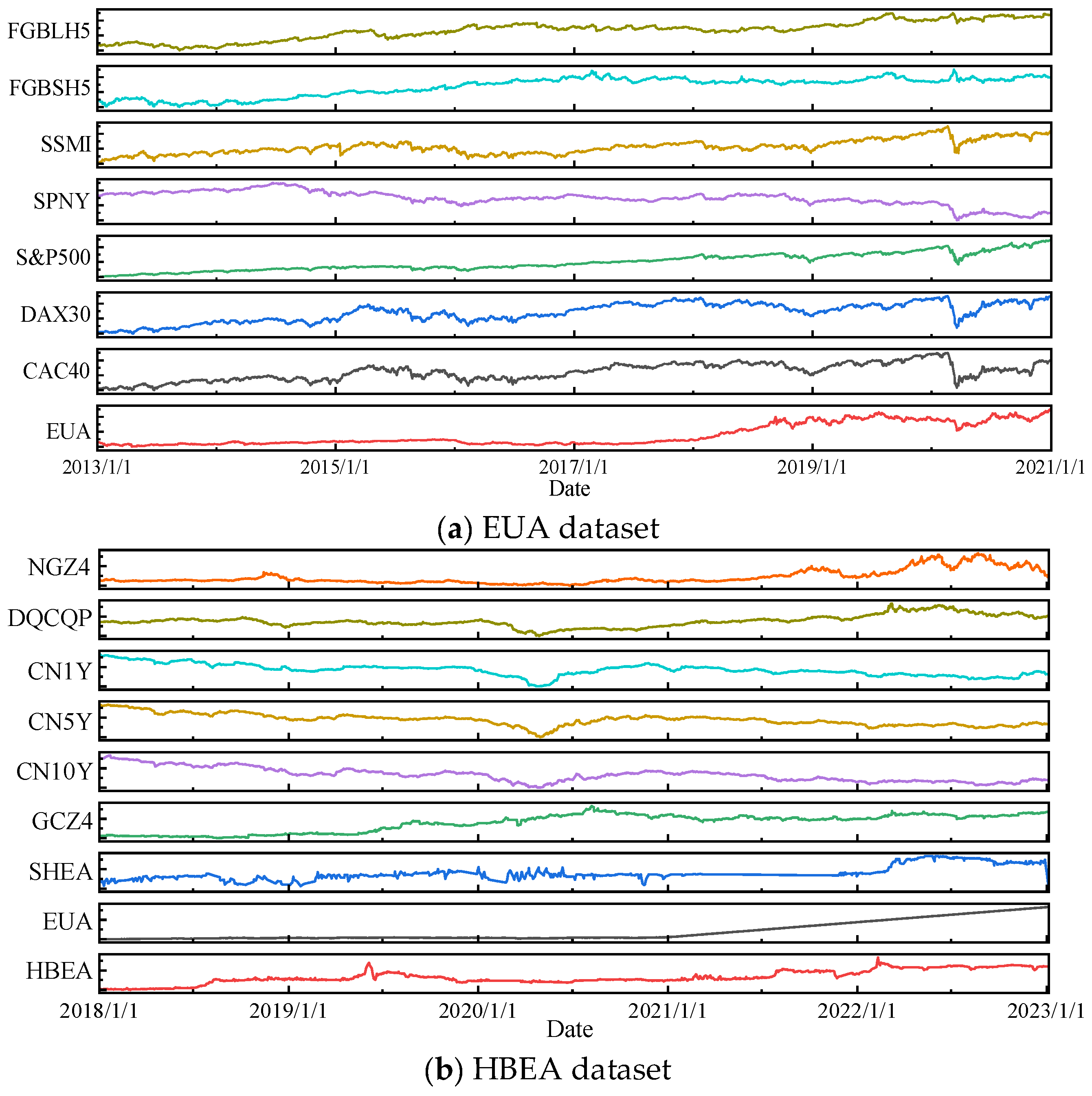
For the collected datasets, a simple linear interpolation method is employed to fill a small number of missing values. The statistical characteristics of the two datasets are summarized in Table 1. Each dataset is sequentially divided into training and testing sets at a ratio of 9:1. The carbon price trends are illustrated in Figure 1. The skewness and kurtosis values of both the EUA and HBEA datasets indicate slight asymmetry and a relatively flat distribution. However, the large standard deviations reflect considerable volatility, suggesting that the data cannot be assumed to be stationary.
This study further evaluates the stationarity and linearity of the datasets using the Augmented Dickey–Fuller (ADF) test and the Brock–Dechert–Scheinkman (BDS) test, respectively. The results are presented in Table 2. The ADF test yields a test statistic of 0.412 and a p-value of 0.982 for the EUA dataset, and a test statistic of −1.511 with a p-value of 0.528 for the HBEA dataset—both p-values significantly exceed the 0.05 threshold, indicating non-stationarity. The BDS test results show large test statistics and p-values of 0 across embedding dimensions from 2 to 5 for both datasets, confirming the presence of nonlinear dependence. These findings demonstrate that carbon price data exhibit both non-stationary and nonlinear characteristics, making accurate forecasting particularly challenging. Therefore, this study applies signal decomposition techniques such as Variational Mode Decomposition (VMD) and Empirical Wavelet Transform (EWT), which are well-suited for handling non-stationary and nonlinear time series, to enhance the prediction of carbon prices.

2.3. Correlation Analysis

Carbon prices are influenced by a variety of factors, including energy, economic, and environmental indicators. A high correlation between two independent variables, known as multicollinearity, can be problematic because it can inflate the variance of the model’s coefficients, making the model less stable and interpretable. Detecting and addressing multicollinearity through techniques like variable selection, dimensionality reduction, or regularization ensures that the model is more reliable and that the predictions are more accurate [30]. This study selects multiple relevant influencing variables and employs Pearson correlation analysis to quantitatively assess the relationship between these variables and carbon prices. To optimize the model’s input variables, the Extremely Randomized Trees (ET) method [31] is employed to assess the grey relational degree between each variable and both the EUA and HBEA carbon prices. By analyzing the SHAP (Shapley Additive explanations) values, the contribution of each variable within the ET model is quantified. This approach aims to evaluate the significance of external factors in driving carbon price fluctuations. The analysis results are presented in Table 3 and Figure 2.
As shown in Table 3, nearly half of the external factors in both datasets exhibit a correlation coefficient greater than 0.5 with carbon prices. Among them, the S&P 500 Index has the highest correlation coefficient of 0.874 with the EUA carbon price; the EUA carbon price, in turn, has the highest correlation coefficient of 0.837 with the HBEA carbon price. The collected climate and environmental indicators can be considered negligible. External factors with correlation coefficients exceeding 0.5 also show relatively high importance scores in the Extra Trees (ET) model, and the SHAP analysis results are consistent with these findings. By integrating the correlation coefficients, ET importance scores, and SHAP contribution values, strong theoretical support is provided for using the matrix of external variables with larger indicators as one branch input for the carbon price prediction models of each dataset. The external variables selected for the EUA and HBEA datasets are illustrated in Figure 3. However, the high multicollinearity among external factors may cause challenges in the modeling process. This phenomenon highlights the importance of developing efficient feature selection algorithms aimed at precisely identifying the optimal factors to further optimize the model inputs.

2.4. Data Normalization

To eliminate the dimensional discrepancies among different features in the dataset and to avoid the adverse effects of inconsistent feature scales on model prediction accuracy, this study applies the min-max normalization method to preprocess the data. The core idea of this method is to use the maximum and minimum values of the data as references and linearly transform the original data range to a unified scale. Specifically, the data are mapped onto the interval [−1, 1], aiming to remove the influence of dimensional differences on feature weights, thereby improving the training performance and prediction accuracy of the model. The corresponding formula is expressed as
X norm = 2 X X min X max X min 1
where X denotes the original data, X norm represents the normalized data, X min is the minimum value in the dataset, and X max is the maximum value in the dataset.

2.5. Modal Decomposition

Variational Mode Decomposition (VMD) is an adaptive signal decomposition method that effectively handles non-stationary and nonlinear signals. By iteratively searching for variational modes, VMD decomposes the original time series into a set of sub-signals with limited bandwidths, each associated with a specific center frequency [32].
Empirical Wavelet Transform (EWT), which integrates Fourier spectrum analysis with wavelet decomposition, addresses the limitations of both methods. It segments the frequency spectrum based on local extrema in the Fourier amplitude and constructs a set of wavelet filter banks for each segment. This allows the original signal to be decomposed into amplitude-modulated and frequency-modulated components across different frequency bands, enabling the extraction of salient modes in both time and frequency domains [33].
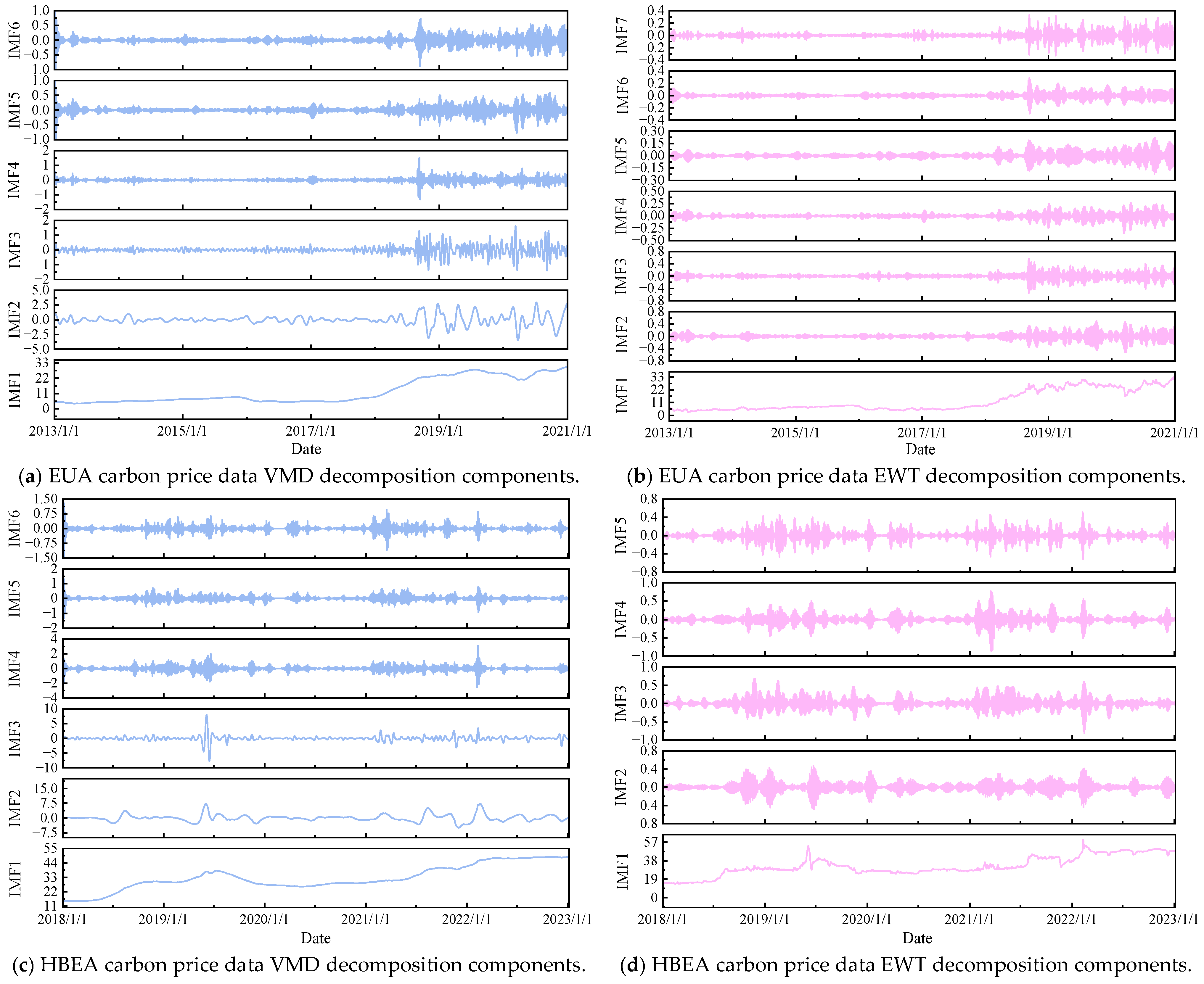
In this study, VMD and EWT are applied to decompose carbon price data from different carbon markets to enhance the prediction performance of deep learning models. As shown in Figure 4, VMD decomposes EUA and HBEA price series into six intrinsic mode functions (IMFs), effectively extracting frequency-specific features, reducing noise and mode mixing, and improving the model’s ability to capture trends and nonlinear dependencies—thereby enhancing both accuracy and robustness. EWT adaptively segments the frequency spectrum and generates seven and five physically interpretable IMFs for the EUA and HBEA datasets, respectively. These components precisely characterize high-frequency transient fluctuations caused by abrupt price changes and extract amplitude–frequency modulation signals, uncovering key patterns in carbon price dynamics. Particularly during periods of volatility, EWT enhances the time-frequency representation of signals. After decomposition, the original series exhibits more distinguishable trends, periodicities, and noise components. Compared to the raw sequence, these transformed components allow clearer identification and analysis of carbon price movements. Therefore, the multi-channel subcomponent matrices obtained via VMD and EWT are fed in parallel into the deep learning model, forming a frequency–time dual-driven feature space. This enables joint exploration of high-frequency details and low-frequency trends, providing rich multidimensional features for accurate carbon price forecasting under complex environments.

3. Deep Learning Model and Prediction Process

3.1. TKMixer Module

For multivariate time series forecasting based on historical data, reference [13] proposes an innovative architecture called TSMixer, which enables efficient modeling by alternately applying multilayer perceptions (MLPs) in both the temporal and feature dimensions. Reference [34] proposed a novel neural network architecture, KAN, based on the Kolmogorov–Arnold theorem. Its breakthrough lies in the introduction of learnable marginal activation functions. This design departs from the conventional multilayer perceptron (MLP) paradigm, where fixed activation functions are assigned to nodes, by instead associating activation functions with network edges (i.e., weights) and endowing them with learning capability. This shift not only enables independent nonlinear transformations along each coordinate axis but also constructs multidimensional mappings by combining these transformations, thus fundamentally differing from the layer-wise uniform nonlinear transformations characteristic of MLPs. The design advantages of a KAN are notable: It supports network sparsification, pruning, and other optimization techniques, thereby enhancing model interpretability and generalization ability. Moreover, this architecture integrates the benefits of spline functions and MLPs, maintaining high precision in low-dimensional spaces while effectively adapting to the complexity of high-dimensional spaces, demonstrating outstanding representational power.
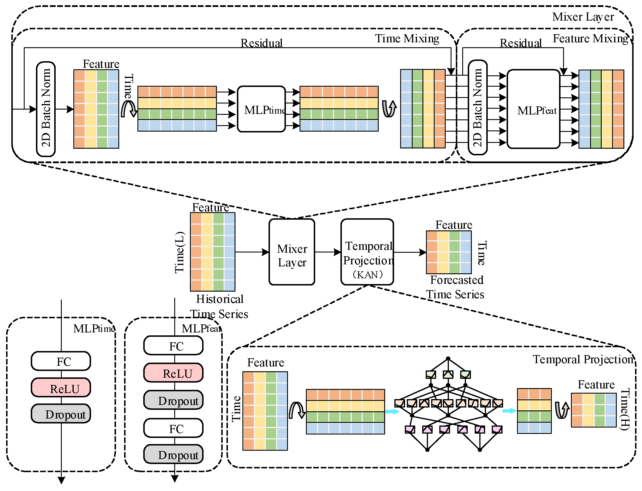
For the carbon price prediction task, this study leverages the strengths of both TSMixer and KAN in mining temporal features, by embedding KAN into the time-mapping layer of the traditional TSMixer module, thus designing the TKMixer module, as illustrated in Figure 5. This module primarily consists of the following core components:
Temporal Mixing MLP: This module is designed to capture temporal patterns within time series data. It employs a structure consisting of fully connected layers, activation functions, and dropout layers. By transposing the input, the fully connected layers are applied along the time axis, allowing feature-wise parameter sharing. Studies have shown that even simple single-layer MLPs can effectively learn complex temporal dependencies through linear transformations. Specifically, let the historical observations be represented as X R L × C x , where L is the length of the input time window and Cx is the number of input variables. The forecasting target is Y R T × C y where T is the number of future time steps to predict, and Cy denotes the number of output variables, CyCx. The linear model predicts the feature values for T time steps by learning the parameters ( A R T × L ) and the bias term ( b R T × 1 ), as follows
Y ^ = A X b R T × C x
where denotes column-wise addition and the corresponding Cy columns in Y ^ are used for prediction.
For any periodic function x t = x t P with period P < L, the linear model can effectively predict its future values, as shown below:
A i j = 1 ,     n = L P + i mod P 0 ,     n L P + i mod P ,     b i = 0
When extended to periodic sequences under affine transformations, i.e., x t = a x t P + c , where a , c R , the linear model can still achieve perfect prediction:
A i j = a ,     n = L P + i mod P 0 ,     n L P + i mod P ,     b i = c
Feature Mixing MLP: This module shares weights across all time steps to fully exploit covariate information. A two-layer MLP architecture is adopted, similar to transformer-based models, to learn complex feature transformation relationships and enhance the model’s understanding of time series patterns.
Residual connections: TSMixer introduces residual connections between each temporal and feature mixing layer to improve learning efficiency in deep architectures, prevent gradient explosion, and enhance information flow. Additionally, this design allows the model to bypass less important temporal or feature mixing operations when necessary, thereby improving computational efficiency and generalization performance.
Normalization: Normalization is a key technique for optimizing deep learning model training. Although the choice between batch normalization and layer normalization depends on the specific task, batch normalization performs better on common time series datasets. Unlike traditional normalization along the feature dimension, this work applies 2D normalization across both temporal and feature dimensions, in coordination with the temporal and feature mixing operations, to improve model stability and generalization.
Time mapping: KAN is used as a substitute for the fully connected layer in the traditional TSMixer framework, applying the KAN architecture to learn complex nonlinear relationships within temporal data and perform time-domain projection. By capturing the long-term dependencies between historical carbon price inputs and future forecasts, it maps the input time feature sequence of length L to a secondary length H, thereby enabling efficient mixing and transformation of carbon price data features.
KAN integrates nonlinear activation functions into the traditional TSMixer module, resulting in smoother parameter representations that enhance both model accuracy and interpretability [35]. The computation process is formulated as follows
f x = q = 1 2 n + 1 φ q p = 1 n ϕ q , p x p
where f x denotes the function output; 2 n + 1 is the upper limit of the outer summation and is related to the input dimension; n ; x p represents the p component of the input vector x with the domain 1 ~ n ; ϕ q , p x p is the inner function representing a composition of the q and p terms; and φ q denotes the outer function corresponding to the q term of the outer summation.
A single KAN layer can thus be expressed as a one-dimensional function matrix:
φ = ϕ q , p , p = 1 , 2 , n i n ,   q = 1 , 2 , n o u t
To construct a deep KAN network by simply stacking multiple KAN layers, the transition matrix between the input and output layers can be expressed as
x l + 1 = ϕ l , 1 , 1 ( ) ϕ l , 1 , 2 ( ) ϕ l , 1 , n l ( ) ϕ l , 2 , 1 ( ) ϕ l , 2 , 2 ( ) ϕ l , 2 , n l ( ) ϕ l , n l + 1 , 1 ( ) ϕ l , n l + 1 , 2 ( ) ϕ l , n l + 1 , n l ( ) x l
where ϕ l denotes the matrix function corresponding to the l KAN layer, and ϕ l , i , j represents the activation function on each edge, which performs the nonlinear transformation. The number of nodes in each KAN layer is determined by the number of input nodes. Consequently, the cascading relationship of multiple layers can be expressed in matrix form as
KAN x = φ L 1 φ L 2 φ 1 φ 0 x
where KAN x denotes the output of the KAN network; φ L represents the function matrix corresponding to the Lth KAN layer; and indicates the composition of inter-layer connections and functions.

3.2. BiGRU Module

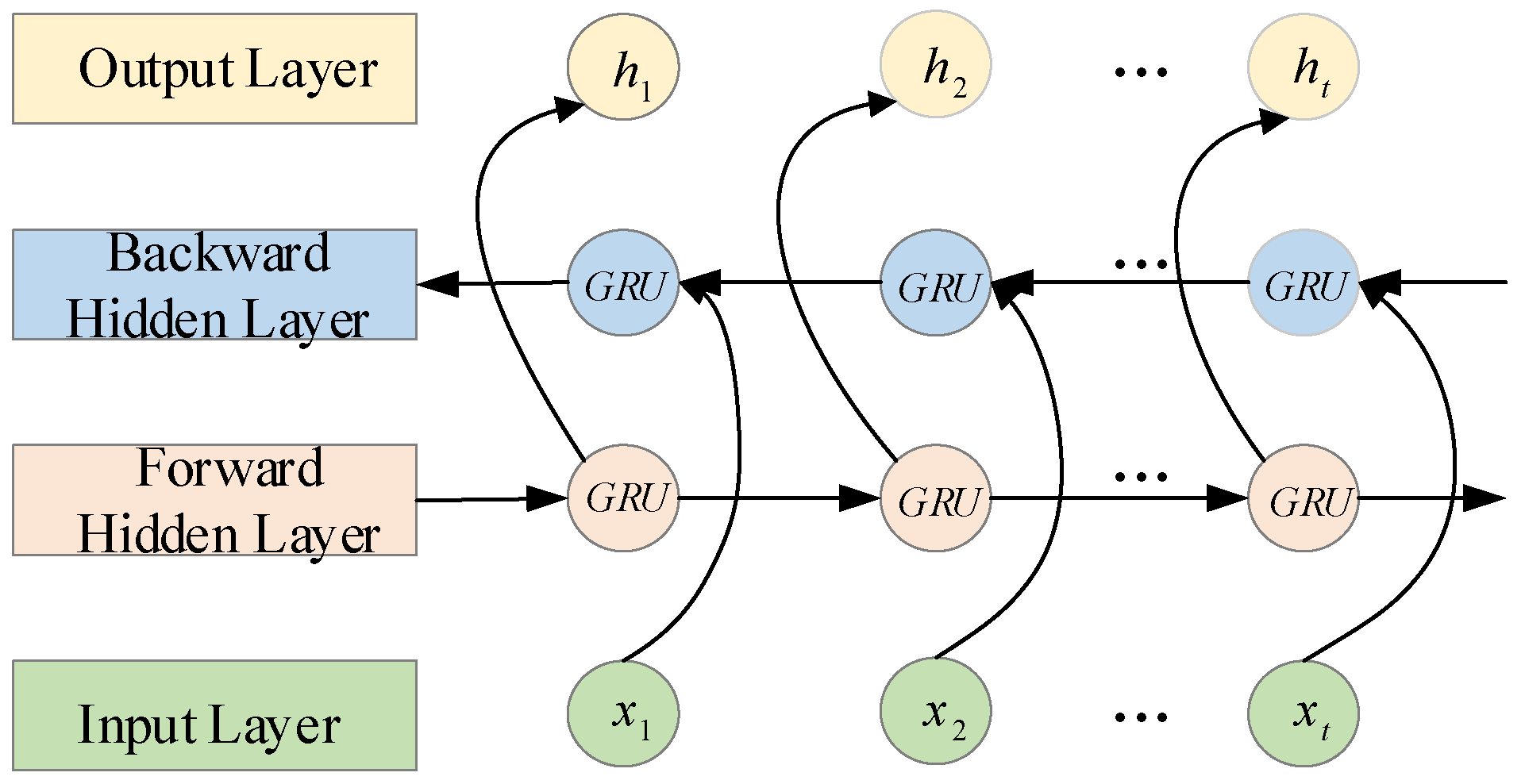
The Gated Recurrent Unit (GRU) primarily consists of a reset gate and an update gate. The reset gate facilitates the capture of short-term dependencies in time series data, while the update gate aids in modeling long-term dependencies. The structure of the GRU is illustrated in Figure 6. The computational process is described by the following equations: The architecture of a KAN typically involves decomposing the input space along each dimension, then processing each component with univariate functions before aggregating the results. The theorem can be formulated as
h t = G R U x t , h t 1 h t = G R U x t , h t 1 Y t = α t h t + β t h t + b t
where α t and β t represent the hidden layer output weights for the forward and backward propagation of the GRU unit at time step t , respectively, and b t denotes the bias corresponding to the hidden state at time step t .
The Bidirectional Gated Recurrent Unit (BiGRU) extends the standard GRU by integrating two independent GRU hidden layers processing the sequence in forward and backward directions, respectively. The forward layer scans the sequence in chronological order, while the backward layer scans it in reverse order, enabling the model to capture both past and future contextual information. This bidirectional structure enhances the ability to learn long-term dependencies and extract deep features. The architecture is illustrated in Figure 7.
BiGRU is a combination of two unidirectional GRU models. Therefore, the output Y t at time step t is obtained from the weighted sum of the forward hidden layer output h t , the backward hidden layer output h t , and a bias term.

3.3. SA Model

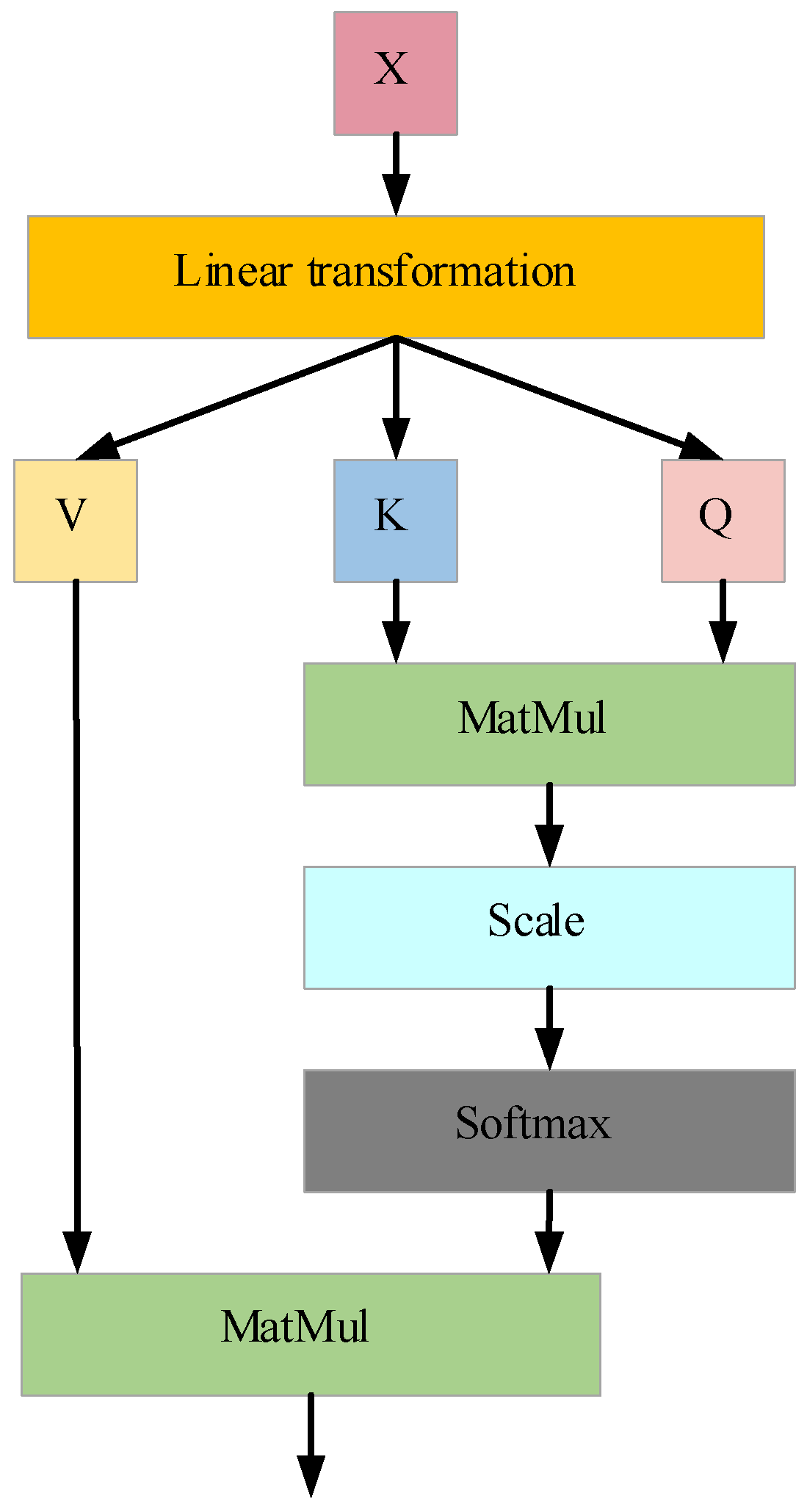
In deep learning, the input to a neural network often consists of multiple vectors that contain potential interdependencies. However, local learning processes between layers may overlook these correlations. To address this issue, the Self-Attention (SA) mechanism has been introduced. SA dynamically adjusts weights to emphasize key features and suppress redundant ones, thereby enhancing the model’s ability to understand and process complex information. The structure is illustrated in Figure 8. The SA mechanism is mathematically expressed as
A t t e n t i o n Q , K , V = s o f t max Q K T d k V
where Q , K , and V represent the query vector, key vector, and value vector, respectively; d k denotes the dimension of the key vector K .

3.4. TKMixer-BiGRU-SA Model

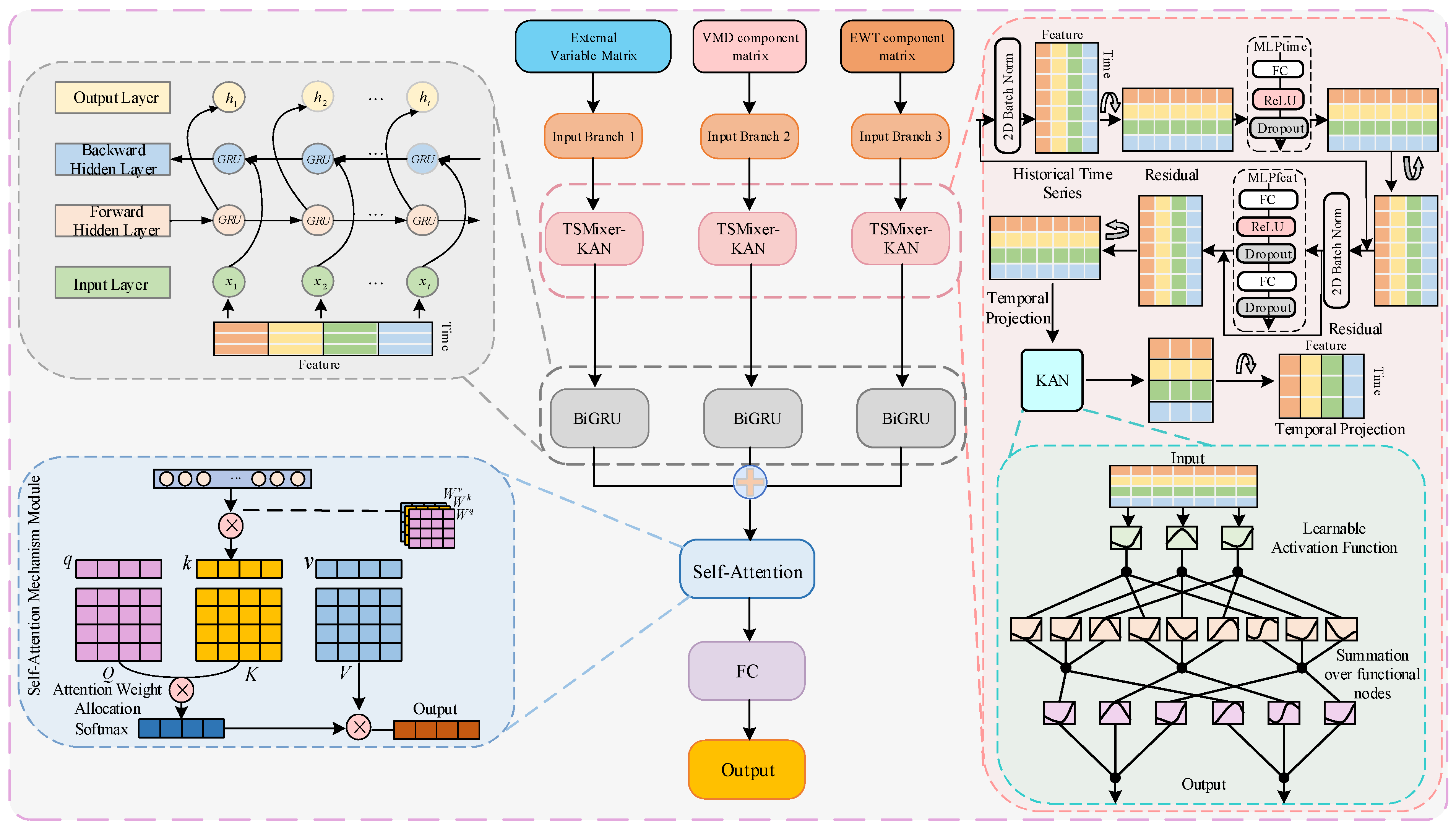
To address the challenge of feature extraction from carbon price data and strongly correlated external factors, this paper proposes a multi-branch input TKMixer-BiGRU-SA carbon price prediction model based on a hybrid decomposition of VMD and EWT, as illustrated in Figure 9.
The proposed model employs a three-branch parallel input architecture. Each branch first applies time series modeling using TSMixer, which utilizes fully connected layers to facilitate interactions across both temporal and feature dimensions, thereby enhancing the modeling of temporal dependencies and feature representations. To further boost expressiveness, a Kolmogorov–Arnold Network (KAN) module is embedded within the temporal mapping layer of TSMixer. This allows for hierarchical nonlinear transformations across time and feature axes, enabling flexible extraction of high-order features. The transformed outputs are subsequently processed by a Bidirectional Gated Recurrent Unit (BiGRU), which captures bidirectional contextual information and strengthens long-term dependency modeling. Following this, a Self-Attention (SA) mechanism is applied to adaptively reweight and fuse features from all input branches. The fused representation is then passed through a fully connected layer to produce the final carbon price prediction. Through this multi-level feature extraction and fusion strategy, the model effectively enhances predictive accuracy for carbon price forecasting.

3.5. Forecasting Process

The proposed carbon price prediction method, based on dual-modal decomposition and the TKMixer-BiGRU-SA architecture, comprises two main stages: data processing and analysis, and model training and prediction evaluation.
In the data processing and analysis stage, missing values are first filled using standard linear interpolation. Then, the correlation coefficients between external factors and carbon prices are calculated. External factors with correlation coefficients greater than 0.5 are selected, and a feature matrix composed of carbon prices and these strongly correlated external factors is constructed as one of the model’s input branches. Meanwhile, the carbon price data from different datasets are decomposed using Variational Mode Decomposition (VMD) and Empirical Wavelet Transform (EWT), and the resulting component matrices serve as the other two input branches. These three input branches are ultimately fed into the TKMixer-BiGRU-SA deep learning model.
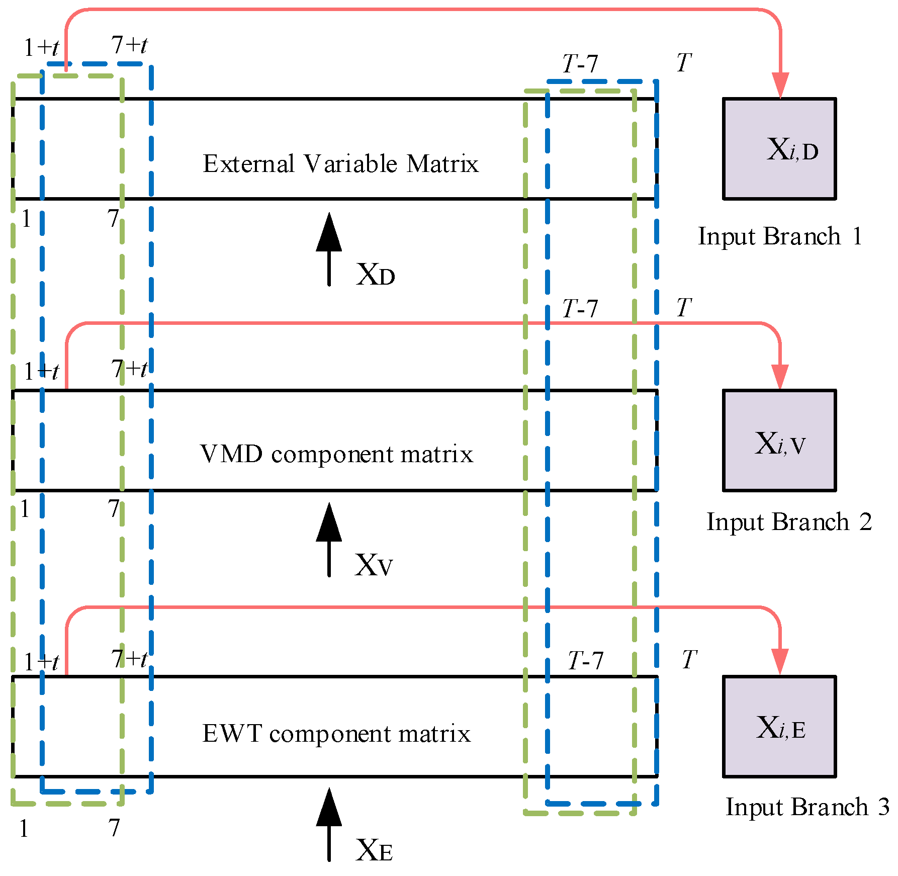
The proposed TKMixer-BiGRU-SA model architecture constructs three distinct feature matrices. Input matrix XD for Branch 1 consists of fused data from EUA and HBEA carbon prices along with external factors showing a correlation above 0.5. Input matrices XV and XE for Branches 2 and 3 are obtained by applying VMD and EWT, respectively, to the EUA and HBEA carbon price data.
For the prediction process, a sliding time window approach is used, with each input unit composed of seven time points. Three step sizes—1, 2, 3, and 4—are employed to construct input matrices of size 7 × N, where N denotes the number of features. In terms of dataset division, the last 10% of each dataset is designated as the test set, while the remaining 90% is used for training.
During sliding prediction, the model uses a 7 × N matrix from the time step immediately preceding point i to predict carbon prices for the interval from point i to i + t − 1, where t is the prediction step size. After each prediction, the model shifts the window to use a new 7 × N matrix from the time step before point i + t as the next input, enabling continuous rolling forecasts. Figure 10 illustrates the sliding window training and prediction process under different step sizes t.
For the model training and prediction evaluation stage, the data processing workflow is illustrated in Figure 11. The TKMixer-BiGRU-SA model, leveraging a multi-module collaborative mechanism, efficiently extracts and integrates multi-scale temporal features from carbon price data and strongly correlated external factors, thereby enhancing prediction accuracy. The detailed process is as follows:
(1)
The TKMixer module primarily processes time series data through two MLP structures: temporal mixing and feature mixing. The KAN network is embedded within the temporal mapping layer to perform hierarchical nonlinear transformations on the features, enabling the flexible extraction of high-order features and enhancing the model’s representational capacity.
The Temporal Mixing MLP operates along the temporal dimension, processing each feature channel independently to capture temporal dependencies. The computation process is as follows
X 1 = L N X X T = σ ( X 1 W n ) X T = X + X T
where the input matrix X R n × j (where n is the number of time steps and j is the feature dimension) corresponds to inputs from the three branches: XD, XV, and XE, respectively. W n R n × n denotes the temporal mixing weights; σ is the activation function (GELU is used in this paper); LN represents the layer normalization function; and the residual connection (+) denotes element-wise addition.
The Feature Mixing MLP operates along the feature dimension, transforming the feature vector at each time step to model inter-variable relationships. The computation process is as follows
X 2 = L N X T X C = σ ( X 2 W j ) f x i = X T + X C
where W j R j × j denotes the feature mixing weights and f x i R n × j i = 1 ,   2 ,   3 represents the output of each branch’s TSMixer module. In this study, the output of the TSMixer modules is maintained at the same dimensionality as the input.
In the first step of the KAN module, each neuron performs a linear transformation on the feature matrix output from the TSMixer module
Z = f x i W + B
where W R j × m is the weight matrix that maps the output from dimension j to the hidden layer of dimension m, B R n × m is the bias matrix, and Z R n × m is the result of the linear transformation:
Z i j = k = 1 d x i k ω k j + b j
Unlike MLPs that use fixed activation functions such as ReLU, the KAN introduces a learnable one-dimensional nonlinear function Φ j at this stage:
f H i j = Φ j Z i j
That is, f H = Φ Z , where Φ j is a learnable univariate function applied element-wise to each column of Z:
f H i j = Φ j k = 1 d x i k ω k j + b j
These learnable functions are typically parameterized using piecewise polynomials or small neural networks rather than fixed functions such as ReLU or Sigmoid. The final output of the KAN module is denoted as f H i R n × m .
(2)
For the BiGRU module, an input consisting of an n × m matrix—where each row is an m-dimensional feature vector—is fed into the BiGRU. By leveraging both forward and backward propagation, the model captures dependencies between historical and future data. This enhances the temporal representation of photovoltaic power and associated meteorological variables at each time step. The computation process is as follows
h t i = δ t i W x i f H i + W i h h i t 1 + b i h t i = δ t i W x i f H i + W i h h i t 1 + b i f B i = δ t i W 1 h t 1 + W i h t i
where i = 1, 2, 3, and W x i and W x i are the weight matrices that project the input layer to the forward and backward hidden layers, respectively. f H i denotes the output from the TKMixer module. W i h and W i h are the recurrent weight matrices that map the outputs from the previous time step to the current time step in the forward and backward hidden layers, respectively. b i and b i are the bias vectors for the forward and backward hidden layers. W i and W i represent the weight matrices that project the forward and backward hidden states to the output layer. δ t i denotes the hyperbolic tangent activation function. h t i and h t i are the forward and backward hidden states at time step t for each of the three input branches. The output of the BiGRU module is denoted as f B i . Assuming a batch size of h, the output of each BiGRU branch is a feature matrix of dimension h × n × 2m, meaning that, at each time step, each branch produces an output of dimension h × 2m after passing through the BiGRU module.
(3)
The temporal features fH1, fH2, and fH3, extracted by the BiGRU module, are stacked and fused to obtain the spatiotemporal feature FM of a single carbon price sample (with dimensions h × n × 6m). After a tensor slicing operation, the features from the last time step (i.e., the feature matrix of size h × 6m) are extracted. Then, the Self-Attention mechanism is applied to correlate and interact with the information from different positions in the sequence, enabling a more comprehensive capture of the dependencies within the sequence. This allows for more effective identification and a focus on the key information within the sequence. The computational process is as follows
F M = f H 1 f H 2 f H 3
Q = F M × W q K = F M × W k V = F M × W v F S = s o f t max Q × K T d k V
where the symbol ‘⊕’ denotes the stacking operation applied to the features obtained from each of the three branches. FM represents the one-dimensional long vector formed by the fused features of the three branches. Wq, Wk, and Wv are the weight matrices corresponding to the query, key, and value in the Self-Attention (SA) module, respectively. Q, K, and V represent the query, key, and value matrices within the SA module. The softmax function is used for normalization, T denotes the matrix transpose operation, and dk is the scaling factor for normalization. FPSA represents the feature sequence output from the SA module.
(4)
Finally, the spatiotemporal feature information FSFSFS obtained from the Self-Attention (SA) module is passed through a fully connected layer to output the predicted carbon price Y at each time step.

4. Discussion

All experiments in this study were conducted under the following hardware configuration: CPU (Intel Core i5-13400F, 2.5 GHz), RAM (64 GB), and GPU (RTX 3060, 12 GB). The deep learning models were implemented using PyTorch 1.10.1 within the PyCharm 2024.1.1 environment. The Adam optimizer was employed for model training.
To objectively evaluate the experimental results, this study adopts four error metrics: enhanced Root Mean Square Error (eRMSE), enhanced Mean Absolute Error (eMAE), enhanced Mean Absolute Percentage Error (eMAPE), and the coefficient of determination (R2). The mathematical formulations of these evaluation metrics are defined as follows
e R M S E = 1 n i = 1 n y ^ i y i 2
e M A E = 1 n i = 1 n y ^ i y i
e M A P E = 1 n i = 1 n y ^ i y i y i × 100 %
R 2 = 1 i = 1 n y i y ^ i 2 i = 1 n y i y ¯ i 2
where y ^ i denotes the predicted carbon price, y i represents the actual carbon price, and y ¯ i is the mean of the actual carbon prices.

4.1. Model Parameter Settings

To optimize model performance, this study conducts a systematic experimental analysis of key parameters across different modules.
(1)
Model architecture and parameter configuration
The hidden layer dimension of the TSMixer module influences its capacity to capture both temporal and feature-level representations, which in turn affects the KAN module’s ability to extract deep correlations from the feature matrix. Second, the hidden layer size of the KAN module directly impacts the model’s ability to extract high-order features. Additionally, the number of neurons in the BiGRU module must strike a balance between effectively capturing bidirectional long- and short-term dependencies and maintaining computational efficiency, thereby ensuring high prediction accuracy without overfitting or excessive resource consumption. Based on these considerations, multiple sets of comparative experiments were designed to test combinations of hidden layer dimensions in the TSMixer and KAN modules, as well as different neuron counts in the BiGRU module. The optimal configuration for each module was determined based on experimental results. With a learning rate of 0.001, a batch size of 16, and 200 training epochs, the evaluation metrics and prediction errors for the one-step carbon market price prediction experiment on the EUA dataset are presented in Table 4 and Figure 12.
As shown in Table 4 and Figure 12, the proposed TKMixer-BiGRU-SA model achieves the lowest error evaluation metrics and the prediction errors are closest to zero when the hidden layer dimensions of the TSMixer and KAN modules are set to 16 and 32, respectively, and the number of neurons in the BiGRU module is set to 32. These results indicate that the model delivers the best prediction performance under this configuration, demonstrating the strongest overall feature extraction capability and the most appropriate parameter settings.
(2)
Model training hyperparameter configuration
Hyperparameters have a significant impact on the training performance and effectiveness of the model. Different combinations of hyperparameters can lead to notable differences in accuracy, convergence speed, and overall model behavior. By conducting comparative experiments, we can systematically and comprehensively evaluate the influence of various hyperparameter settings, visually compare the advantages and disadvantages of each combination, and accurately identify the configuration that yields optimal model performance on a specific task and dataset. The experimental results under the optimal model parameters with different training hyperparameter settings are shown in Table 5, and the training loss curves are illustrated in Figure 13.
The experimental results indicate that appropriately increasing the number of training epochs (epoch = 200) significantly improves performance. The combination of batch size = 16 and learning rate = 0.001 achieves the best trade-off between error and model fitting, yielding the lowest eRMSE (0.0648) and the highest R2 (0.9997), while maintaining good training efficiency (323 s). In contrast, an excessively large batch size or an overly small learning rate leads to performance degradation. Overall, the 200-16-0.001 configuration proves to be the optimal and most stable setting, demonstrating a favorable balance between training efficiency and prediction accuracy.

4.2. Comparison Experiment with Different Inputs

To verify the effectiveness of the selected feature variables and the combined input strategy based on decomposition methods, a series of experiments were designed as follows:
B1: uses the original carbon price data as a single-branch model input.
B2: builds upon B1 by adding relevant feature variables filtered through Pearson correlation analysis, still using a single-branch input.
B3: extends B2 by incorporating the VMD-decomposed components of the original carbon price series, forming a dual-branch model input.
B4: builds upon B2 by introducing EWT-decomposed components of the original carbon price series, maintaining a dual-branch structure.
B5: builds upon B2 by introducing CEEMDAN-decomposed components of the original carbon price series, maintaining a dual-branch structure
B0: combines the inputs from B2, B3, and B4 to form a full three-branch model input.
Traditional model frameworks have primarily focused on single-step prediction, where deep learning models infer the next day’s carbon price based solely on historical closing prices. However, multi-step prediction offers a significant advantage by uncovering longer-term trends in price dynamics, providing broader and more strategic insights for market decision-making.
To assess the model’s performance in multi-step forecasting scenarios, this study employs carbon price data from the EUA and HBEA markets and conducts forward prediction experiments for two-step, three-step, and four-step horizons. Specifically, two-step forecasting aims to estimate the carbon prices for the two trading days following the end of the training set; three-step and four-step forecasts extend this prediction window accordingly.
All experiments were conducted using the proposed TKMixer-BiGRU-SA model and its core variants. The prediction errors on the test sets for both datasets are presented in Table 6, and the linear regression results between predicted and actual values are shown in Figure 14.
The analysis results indicate that under the forecasting scenarios 1–4 steps ahead, prediction accuracy generally declines as the forecasting horizon increases. However, compared to other input configurations, the proposed input strategy in experiment B0 consistently yields the lowest error levels across all forecast lengths. Furthermore, analysis of the normal distribution of prediction errors across different prediction step sizes shows that B0 achieves the smallest mean and standard deviation of errors, indicating higher model stability and reliability. These findings provide strong evidence supporting the predictive capability of the proposed model.
For the EUA dataset, Experiment B0 outperforms all other configurations across the four evaluation metrics. Specifically, in the one-step forecast, the model achieves an eRMSE of 0.0648, an eMAE of 0.0504, an eMAPE of 0.2081%, and an R2 of 0.9997, demonstrating high prediction accuracy and an excellent fit. In the four-step forecast, comparative experiments B1 through B5 demonstrate the effectiveness of various input configurations. Compared with B1, B2 achieves a 1.127% reduction in eMAPE and a 0.6459% improvement in R2, indicating that the inclusion of relevant variables enhances the model’s sensitivity and accuracy by providing a more comprehensive representation of carbon price dynamics. Further, B3 and B4 show significant improvements over B2, with eMAPE reductions of 51.732% and 12.8966%, and R2 increases of 6.3309% and 1.7840%, respectively. These results indicate that the introduction of VMD and EWT decomposition branches substantially enhances prediction performance. The VMD algorithm effectively decomposes nonlinear and non-stationary signals, while the EWT algorithm extracts amplitude- and frequency-modulated components, both of which help uncover the intrinsic patterns of carbon price fluctuations. Although B5 shows relatively high performance metrics compared to B3 and B4, its slightly inferior accuracy suggests that CEEMDAN, despite decomposing the original signal into a greater number of components, may introduce additional noise-like disturbances, leading to overfitting and reduced prediction precision. Compared with B3 and B4, B0 achieves eMAPE reductions of 33.3514% and 63.0667%, and R2 increases of 1.4629% and 5.9955%, respectively. These results underscore that integrating additional input data leads to a more comprehensive and accurate predictive model.
For the HBEA dataset, similar trends are observed, further validating the superiority of the three-branch input structure. In the one-step prediction experiment, configuration B0 achieved the best performance across all four metrics—eRMSE, eMAE, eMAPE, and R2—registering values of 0.0884, 0.0664, 0.1389%, and 0.9968, respectively. The worst performance was observed in B1 and B2, differing from the results on the EUA dataset. This discrepancy may stem from the developmental stage of the Hubei carbon market, which is likely less mature and characterized by relatively simpler and more stable price dynamics. Furthermore, Hubei’s market data may be influenced by factors such as policies, quota allocations, and enterprise behavior. In this context, VMD and EWT decomposition techniques can effectively extract more critical features from the raw data, thereby improving prediction accuracy.
In summary, the proposed dual-modal decomposition tri-branch input model achieves higher forecasting accuracy and lower prediction error, effectively demonstrating the validity of the improved input strategy and providing a strong foundation for future forecasting research.

4.3. Ablation Experiment

To evaluate and understand the importance of each module within the deep learning model and its impact on overall performance, this study conducts ablation experiments. By observing how modifications to the model structure affect its performance and outputs, the goal is to identify the most optimized architecture, improve efficiency, and enhance the interpretability of the proposed TKMixer-BiGRU-SA model. The experimental configuration is as follows:
C1: TSMixer.
C2: TKMixer.
C3: BiGRU.
C4: TKMixer-BiGRU.
C0: TKMixer-BiGRU-SA (proposed model).
Configuration C1 and C3 represent baseline models using only the TSMixer or BiGRU modules, respectively, within the three-branch deep learning architecture. C2 embeds the KAN network into the temporal mapping layer of the TSMixer module. C4 combines the modules from C2 and C3 in a deep sequential structure within the same branch. C0, the complete model proposed in this study, extends C4 by integrating a Self-Attention (SA) module to validate the significance of attention mechanisms in optimizing model performance and improving prediction accuracy.
Table 7 presents the performance metrics of the model architectures under different ablation experiment configurations. As shown, the models in experiments C1 and C3, which adopt a single basic module, exhibit relatively low parameter counts and floating-point operations, resulting in faster training. This efficiency is primarily attributed to the simplicity of the module structures. However, these configurations demonstrate limited feature extraction capability, leading to lower prediction accuracy. In contrast, experiments C2 and C4 incorporate both the KAN and BiGRU modules, which significantly enhance the model’s ability to capture complex data features. This improvement, however, comes at the cost of increased model parameters and computational complexity, thus reducing training efficiency. Experiment C0 represents the full model proposed in this study, which integrates the strengths of multiple structural modules. Although this configuration leads to increased model complexity and longer training time, it achieves superior prediction accuracy compared to the other configurations. The increase in computational overhead remains within an acceptable range. Therefore, the moderate trade-off between accuracy and efficiency—achieved through a multi-module collaborative architecture—proves to be a rational and effective design choice.
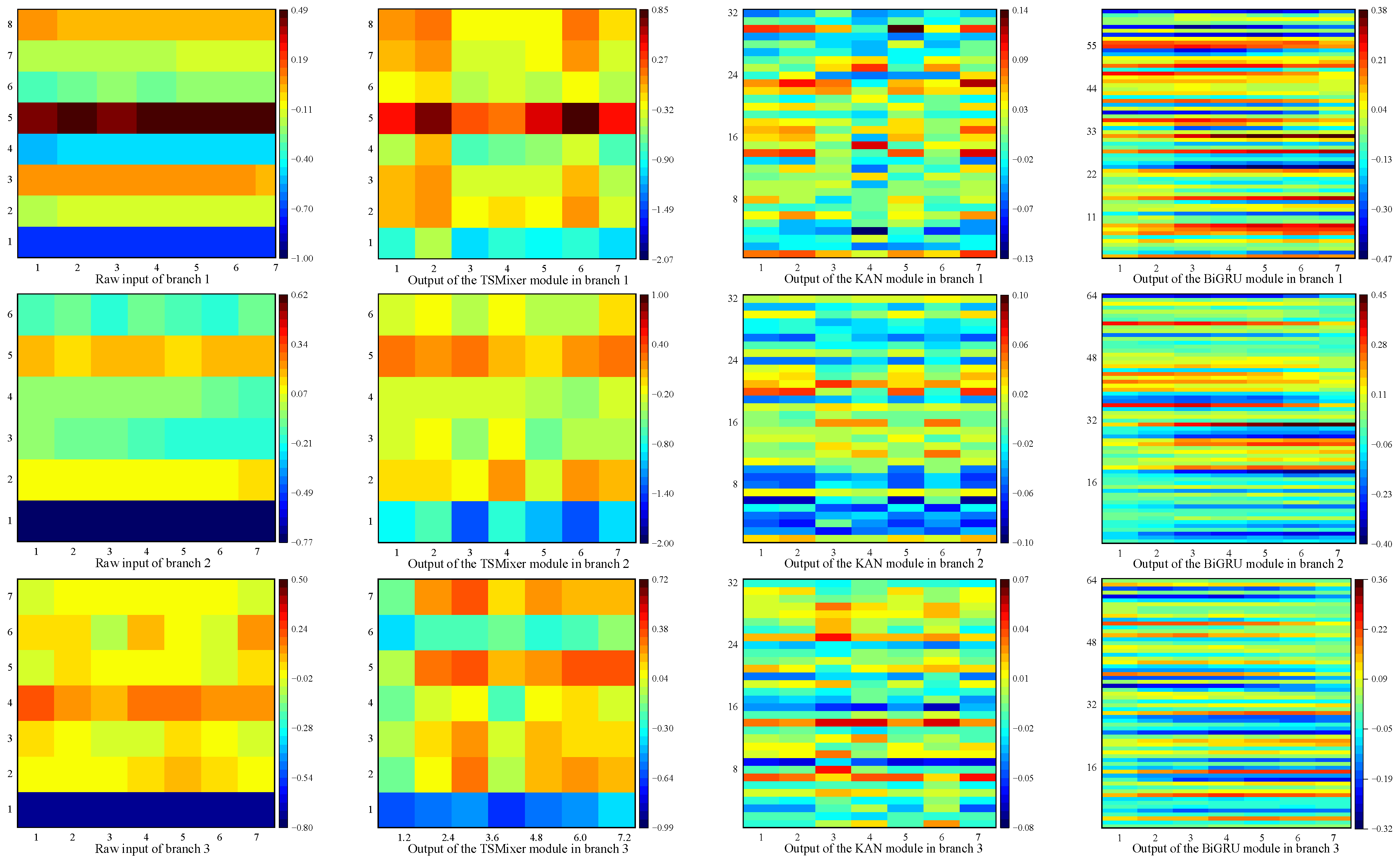
Taking the one-step prediction experiment on the EUA dataset as an example, the features extracted by each module from a single input are visualized using pseudo-color images, as shown in Figure 15. A comparative analysis of the visualized features from the three-branch structure reveals significant differences between the feature maps extracted from the carbon price subcomponent matrix—generated via the hybrid VMD + EWT decomposition—and those extracted from the external factor matrix. This demonstrates the effectiveness of the proposed scheme in capturing multi-scale features inherent in the carbon price data. Under optimal parameter settings, the features extracted by the different modules exhibit considerable variation, indicating that the sequential arrangement of submodules contributes to feature complementarity. This, in turn, provides valuable references for the Self-Attention (SA) module to effectively focus on key temporal features.
All five configurations are trained using the tri-branch input framework. The prediction curves for the test sets of the EUA and HBEA datasets are shown in Figure 16 and Figure 17, respectively, and the corresponding prediction error metrics are summarized in Table 8.
EUA dataset: A comparative analysis between experiments C1 and C2 reveals that integrating the KAN module into the baseline TSMixer architecture significantly improves model performance. Compared to the original TSMixer model, the TKMixer configuration achieves substantial reductions in all error metrics. Specifically, R2 values increase to 0.9986, 0.9962, 0.9915, and 0.9906 across the 1–4 step prediction horizons, validating the effectiveness of the KAN module in extracting high-order features and enhancing feature representation.
Further comparisons between C4 and both C2 and C3 show that, in one-step forecasting, C4 reduces eRMSE by 34.7440% and 42.2007%, eMAE by 11.3200% and 47.6673%, and eMAPE by 31.4208% and 46.3130%, respectively. These results demonstrate that the TKMixer structure enables efficient feature mixing and transformation, strengthening temporal dependencies and expressiveness. When coupled with BiGRU’s bidirectional dependency modeling, the combined architecture accurately captures critical features in the input sequence, leading to significantly improved prediction performance.
C0, the full model incorporating the Self-Attention (SA) mechanism, further enhances prediction accuracy through dynamic weighting of feature importance. Under this configuration, eMAPE drops to 0.2081%, 0.5660%, 0.8293%, and 1.1063% for 1–4 step predictions, while R2 reaches 0.999, 0.9978, 0.9957, and 0.9918, respectively.
As shown in Figure 11, the predicted values from the proposed model closely align with the ground truth, with minimal fluctuations and positioning near the center of the 95% confidence interval for all comparative predictions. The predicted mean curve closely follows that of the true values, while eRMSE, eMAE, and eMAPE all exhibit a clear inward contraction, and R2 shows a pronounced outward expansion. These consistent trends confirm that the proposed model achieves the lowest prediction errors and the highest fit quality, demonstrating superior forecasting performance.
HBEA dataset: The experimental results on the HBEA dataset confirm the performance trends observed in the EUA dataset, further highlighting the robustness and superior predictive capabilities of the proposed model. As shown in Figure 17, during periods of sharp carbon price fluctuations, the proposed model closely fits the actual values. Compared to the TKMixer and BiGRU models, in the one-step forecast, the proposed model reduces eRMSE by 41.9567% and 39.9864%, eMAE by 51.7090% and 49.2355%, and eMAPE by 51.5352% and 48.8586%, while improving R2 by 0.6259% and 0.5650%, respectively.
In contrast to the EUA dataset, the HBEA dataset exhibits more pronounced volatility and uneven historical data distribution, which increases the difficulty of prediction. The TKMixer model tends to underestimate in low-price regions, resulting in larger errors, while the TKMixer-BiGRU model overestimates in high-price regions, also leading to increased errors. In comparison, the proposed model produces predictions that closely follow the actual curve, especially around the average value of the test set, with reduced fluctuations in the fitting line. Moreover, the inward contraction of error metrics such as eRMSE, eMAE, and eMAPE, alongside the outward increase in R2, reinforces that the proposed model yields the lowest prediction errors and the highest degree of fit. However, R2 values for the HBEA test set under 1–4 step forecasts—0.9968, 0.9926, 0.9755, and 0.9726—are slightly lower than those from the EUA dataset. This difference is attributed to the higher complexity and volatility of the HBEA data, as well as external influences such as China’s carbon reduction policies (e.g., mitigation actions, nationally determined contributions, and carbon neutrality goals), which were not explicitly modeled.
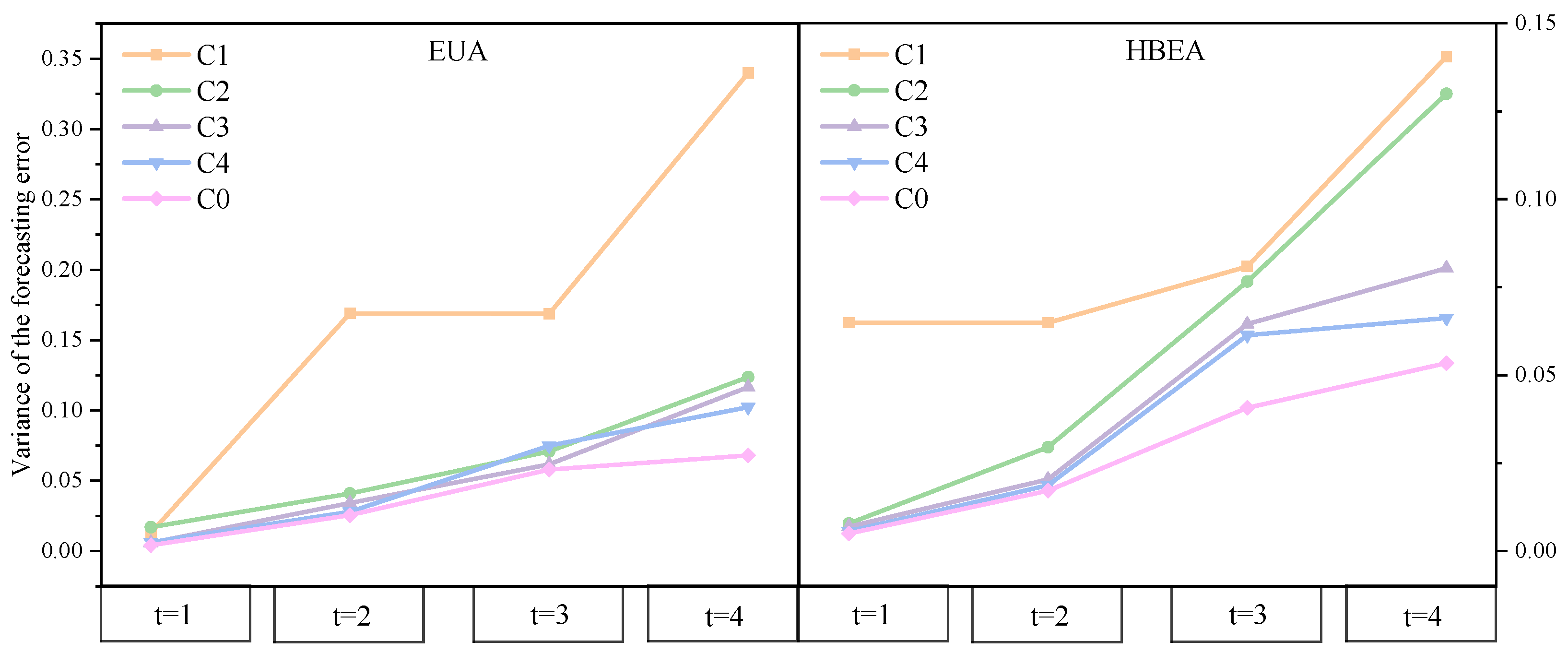
Figure 18 and Table 9 present the variance of prediction errors and the results of paired-sample t-tests across different model configurations on the EUA and HBEA datasets. Variance-based comparative analysis demonstrates that the proposed TKMixer-BiGRU-SA model consistently outperforms others on both datasets, achieving the lowest and most stable error variances across one- to four-step forecasts, thus exhibiting a clear competitive advantage.
The paired-sample t-test results further confirm that integrating the KAN module into the TSMixer architecture (C1 vs. C2) leads to significant improvements in multi-step prediction performance, particularly enhancing stability on the HBEA dataset. This highlights the KAN’s effectiveness in capturing complex temporal dependencies. Moreover, introducing the BiGRU structure (C2 vs. C4) yields notable performance gains at all prediction horizons, validating the importance of bidirectional contextual modeling in sequence prediction.
The combination of TKMixer with BiGRU (C3 vs. C4) also consistently achieves statistically significant improvements, underscoring the synergistic effect between these components as a key driver of model performance enhancement. Building upon C4, the incorporation of the Self-Attention mechanism (C4 vs. C0)—as in the proposed final model—delivers additional performance gains at most time steps, with particularly pronounced improvements at t = 1 and t = 2. This demonstrates the model’s enhanced capacity to focus on critical temporal features. However, minor performance fluctuations observed at a few time steps suggest that the application of attention mechanisms should be carefully tailored to task-specific characteristics.
Overall, these experimental findings validate the effectiveness and robustness of modular composition in improving prediction performance and highlight subtle yet statistically significant differences between competing model architectures.

4.4. Comparison Experiment with Different Literature

To validate the superiority of the proposed forecasting scheme compared to various existing models and methods reported in current research, this study conducted a series of comparative experiments.
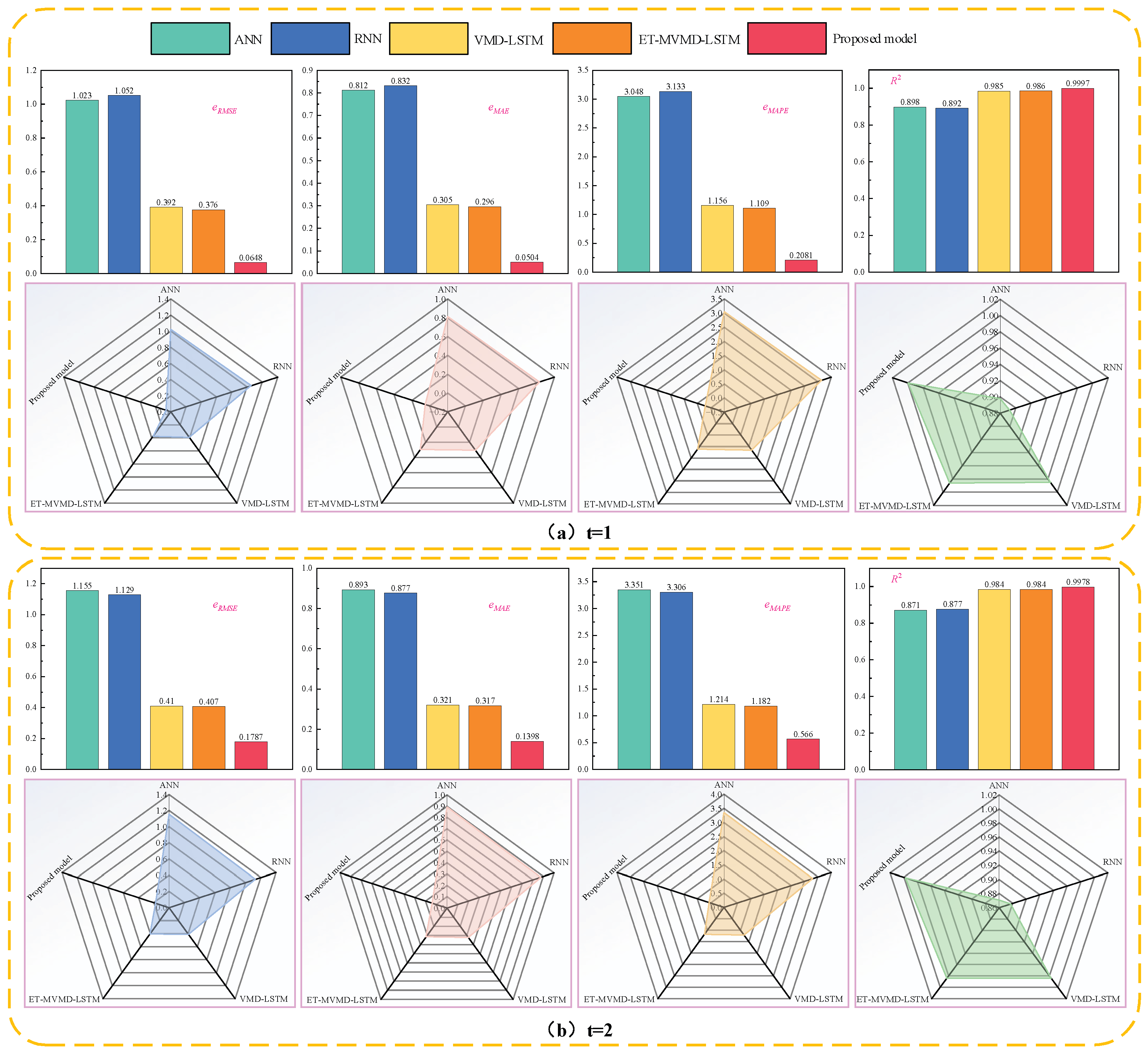
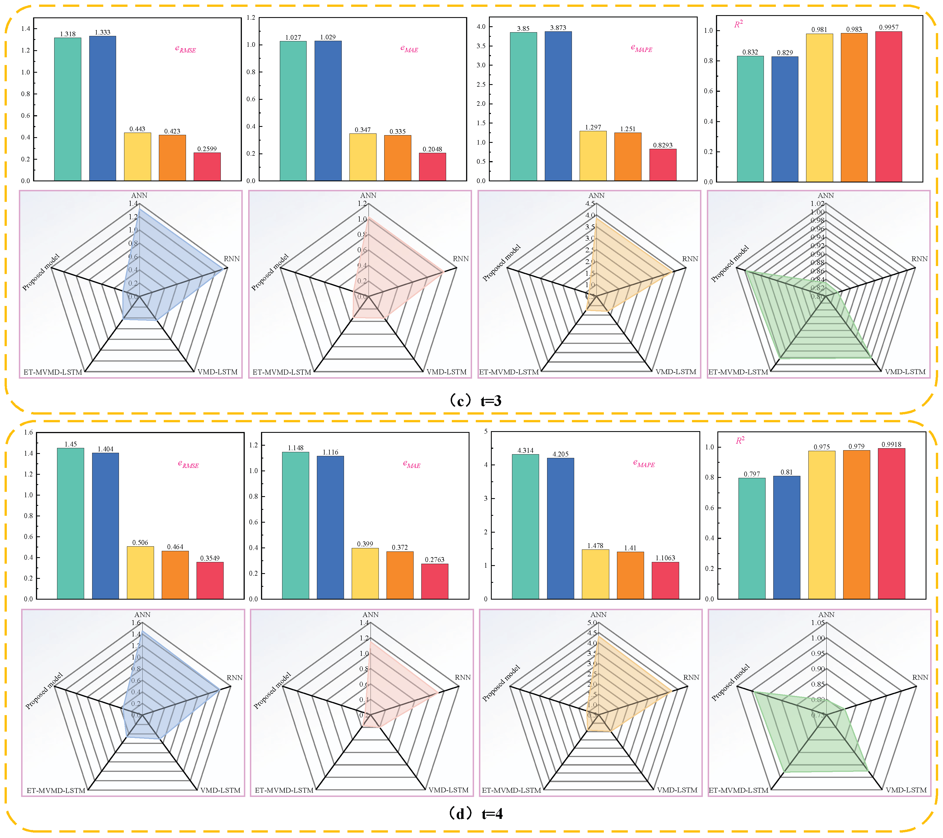
Using the EUA carbon price data from 1 January 2013 to 1 January 2021 as an example, the prediction error metrics of the method presented in [36] and those of the proposed model are compared. As shown in Figure 19, the proposed method demonstrates clear advantages in terms of prediction accuracy across all evaluated metrics.
As shown in Figure 19, the prediction difficulty increases with the forecasting horizon. This is reflected in the rising values of eRMSE, eMAE, and eMAPE, along with a decreasing R2, indicating a decline in predictive accuracy. The ET-MVMD-LSTM hybrid forecasting model proposed in [36] integrates ET-based feature selection, MVMD decomposition, and LSTM deep learning architecture. This approach effectively reduces the complexity of time series data while capturing the inter-variable correlations, enabling it to accurately model the dynamic behavior of carbon prices. It performs well even in multi-step forecasting tasks, demonstrating more stable and reliable performance than single models such as ANN and RNN. Specifically, for one-step forecasting, it achieves an eRMSE of 0.376, eMAE of 0.296, eMAPE of 1.109%, and an R2 of 0.996.
In contrast, the TKMixer-BiGRU-SA model proposed in this study maintains high prediction fidelity across 1 to 4-step ahead forecasts. Notably, for the four-step forecast, the model achieves an eMAPE of just 0.2081% and an R2 of 0.9997. Compared to the ET-MVMD-LSTM model from [36], the eMAPE of our model is reduced by 81.2353%, 52.1151%, 33.7090%, and 21.5390% for 1–4 step predictions, respectively. These results strongly support the effectiveness and robustness of our model in handling complex and challenging prediction tasks.
Regarding the HBEA dataset, Figure 20 presents a comparison of one-step forecasting error metrics between our proposed model and those from [37,38,39]. The TKMixer-BiGRU-SA model consistently achieves the lowest eRMSE, eMAE, and eMAPE, and the highest R2 among all methods. Specifically, compared to the traditional ARIMA model from [37], the proposed model reduces eRMSE, eMAE, and eMAPE by 82.4777%, 82.3591%, and 88.9057%, respectively—highlighting the limited predictive power of single models in capturing complex data features.
By integrating suitable decomposition strategies and leveraging complementary strengths of hybrid deep learning models, our approach effectively utilizes multidimensional features of carbon price data and its external factors, leading to a significant improvement in predictive performance. Compared with the VMD-AWLSSVR-PSOLS-WSM model [37], the HI-TVFEMD-transformer model [38], and the Informer-DABOHBTVFEMD-CL model [39], our method achieves reductions in eRMSE, eMAE, and eMAPE of 50.9433%, 79.4705%, and 58.7879%; 53.5989%, 56.9390%, and 51.3909%; and 70.3142%, 66.1220%, and 52.1034%, respectively. Additionally, the R2 reaches as high as 0.9968. The potential overfitting in previous models may stem from overlapping functionalities and excessive parameter complexity in their hybrid architectures, despite employing signal decomposition techniques. In contrast, our model effectively balances data decomposition and feature extraction, maximizing the performance of each module and validating the soundness of our methodological design.

5. Conclusions

This study proposes a dual-modal decomposition and triple-branch input deep learning model—TKMixer-BiGRU-SA—and successfully applies it to two representative carbon trading market datasets: EUA and HBEA. Based on an extensive cross-comparison of four evaluation metrics, the proposed model consistently demonstrates strong predictive fitting and low forecasting errors across various experimental settings. In single-step forecasting, the model achieves an eMAPE of 0.2081% and an R2 of 0.9997 on the EUA dataset, and an eMAPE of 0.1389% with an R2 of 0.9968 on the HBEA dataset. Moreover, in forecasts 1–4 steps ahead, the model maintains a clear advantage over different decomposition schemes, ablation tests, and alternative approaches, exhibiting notable robustness and accuracy.
(1)
The triple-branch input structure of the deep learning model integrates multiple information sources, enhancing adaptability to complex nonlinear data and improving forecasting performance. Specifically, the first branch preserves the integrity of the original data, capturing direct signals and the latent influence of external factors. The second branch utilizes Variational Mode Decomposition (VMD) to extract frequency-based components, aiding the understanding of data nonlinearity and non-stationarity. The third branch applies Empirical Wavelet Transform (EWT) to obtain intrinsic mode functions (IMFs) with clear physical interpretations, accurately characterizing high-frequency transient fluctuations due to price shocks and isolating amplitude and frequency modulation components.
(2)
The TKMixer-BiGRU-SA architecture integrates the strengths of TSMixer, Kolmogorov–Arnold Networks (KAN), the Bidirectional Gated Recurrent Unit (BiGRU), and Self-Attention mechanisms (SA). A novel contribution of this work is embedding a KAN into the time-mapping layer of the TSMixer module, enabling efficient feature mixing and transformation. This architecture fully captures the temporal dependencies and long-range patterns in time series data while dynamically adjusting the attention to key features. The model exhibits multi-level feature extraction capabilities, contextual understanding, and precise focus on relevant information, thus enhancing generalization and significantly improving carbon price prediction accuracy.
(3)
This study underscores the importance of multi-step ahead forecasting, a topic that remains underexplored in existing research. To address this gap, we conduct comprehensive experiments validating the model’s performance in multi-step prediction scenarios. The results confirm that the TKMixer-BiGRU-SA model delivers strong and consistent performance even in forecasts 1–4 steps ahead, demonstrating its clear advantage and great potential in complex time series forecasting tasks, especially in forward-looking applications.
(4)
In this study, when applying decomposition methods, the training set is decomposed separately first, and then the test set and training set are combined to decompose the entire dataset. Although this approach avoids information leakage from the test set into the decomposition results of the training set, because the entire training set is decomposed together, there still exists the issue of future information leakage during the training phase. Decomposing the whole dataset to obtain the decomposition results of the test set can reduce the endpoint effects on the test set; however, since the entire dataset is decomposed uniformly, some future information leakage inevitably occurs within the test set, so boundary problems still persist [40]. Moreover, due to different time series lengths between separately decomposed training sets and the whole dataset decomposition, differences in decomposition levels may arise. Therefore, further improvements addressing this issue should be made in future research.
(5)
With the advancement of signal processing technologies and deep learning, the combined prediction method proposed in this paper can be further improved or applied to more fields, thereby further demonstrating the research value of the proposed approach.

Author Contributions

Conceptualization, Y.L.; methodology, G.B.; software, Y.L.; validation, Y.L.; formal analysis, N.Y.; investigation, S.C.; resources, Z.L. and X.S.; data curation, G.B.; writing—original draft preparation, Y.L.; writing—review and editing, G.B.; visualization, Y.L.; supervision, N.Y. and S.C.; project administration, Z.L.; funding acquisition, G.B. All authors have read and agreed to the published version of the manuscript.

Funding

This paper was supported by the National Key R&D Program of China (Grant no. 2022YFB2703500).

Data Availability Statement

The codes developed are not public. However, data will be made available on request.

Conflicts of Interest

Author Xin Shen is employed by the Measurement Center of Yunnan Power Grid Co., Ltd. The remaining authors declare that the research was conducted in the absence of any commercial or financial relationships that could be construed as a potential conflict of interest.

References

  1. McMichael, A.J.; Woodruff, R.E.; Hales, S. Climate change and human health: Present and future risks. Lancet 2006, 367, 859–869. [Google Scholar] [CrossRef] [PubMed]
  2. Kazemzadeh, E.; Fuinhas, J.A.; Salehnia, N.; Koengkan, M.; Shirazi, M.; Osmani, F. Factors driving CO2 emissions: The role of energy transition and brain drain. Environ. Dev. Sustain. 2024, 26, 1673–1700. [Google Scholar] [CrossRef]
  3. Qin, B.; Zhou, X.; Ding, T.; Shi, W.; Li, H.; Wen, Y. Review on Development of Global Carbon Market and Prospect of China’s Carbon Market Construction. Dianli Xitong Zidonghua/Autom. Electr. Power Syst. 2022, 46, 186–199. [Google Scholar]
  4. Zhou, K.; Li, Y. Carbon finance and carbon market in China: Progress and challenges. J. Clean. Prod. 2019, 214, 536–549. [Google Scholar] [CrossRef]
  5. Bataille, C.; Guivarch, C.; Hallegatte, S.; Rogelj, J.; Waisman, H. Carbon prices across countries. Nat. Clim. Chang. 2018, 8, 648–650. [Google Scholar] [CrossRef]
  6. Emad, K.; Alberto, J.F.; Narges, S.; Koengkan, M.; Silva, N. Exploring necessary and sufficient conditions for carbon emission intensity: A comparative analysis. Environ. Sci. Pollut. Res. Int. 2023, 30, 97319–97338. [Google Scholar]
  7. Owais, M.; Sayed, E.A.M. Red light crossing violations modelling using deep learning and variance-based sensitivity analysis. Expert Syst. Appl. 2025, 267, 126258. [Google Scholar] [CrossRef]
  8. Shi, H.; Wei, A.; Xu, X.; Zhu, Y.; Hu, H.; Tang, S. A CNN-LSTM based deep learning model with high accuracy and robustness for carbon price forecasting: A case of Shenzhen’s carbon market in China. J. Environ. Manag. 2024, 352, 120131. [Google Scholar] [CrossRef]
  9. Mu, G.; Dai, L.; Ju, X.; Chen, Y.; Huang, X. MS-IHHO-LSTM: Carbon price prediction model of multi-source data based on improved swarm intelligence algorithm and deep learning method. IEEE Access 2024, 12, 80754–80769. [Google Scholar] [CrossRef]
  10. Sayed, G.I.; El-Latif, E.I.A.; Darwish, A.; Snasel, V.; Hassanien, A.E. An optimized and interpretable carbon price prediction: Explainable deep learning model. Chaos Solitons Fractals 2024, 188, 115533. [Google Scholar] [CrossRef]
  11. Wang, M.; Hu, Q.; Zhu, W.; Huang, J. Carbon Price Forecasting for China’s Eight Major Markets Based on GRU-Attention Model. In Proceedings of the 2024 2nd Asia Conference on Computer Vision, Image Processing and Pattern Recognition, Xiamen, China, 26–28 April 2024; pp. 1–6. [Google Scholar]
  12. Zhang, Z.; Liu, X.; Zhang, X.; Yang, Z.; Yao, J. Carbon Price Forecasting Using Optimized Sliding Window Empirical Wavelet Transform and Gated Recurrent Unit Network to Mitigate Data Leakage. Energies 2024, 17, 4358. [Google Scholar] [CrossRef]
  13. Chen, S.A.; Li, C.L.; Yoder, N.; Arik, S.O.; Pfister, T. Tsmixer: An all-mlp architecture for time series forecasting. arXiv 2023, arXiv:2303.06053. [Google Scholar]
  14. Souto, H.G.; Heuvel, S.K.; Neto, F.L. Time-mixing and feature-mixing modelling for realized volatility forecast: Evidence from TSMixer model. J. Financ. Data Sci. 2024, 10, 100143. [Google Scholar] [CrossRef]
  15. Lee, Y.; Jeong, J. TSMixer- and Transfer Learning-Based Highly Reliable Prediction with Short-Term Time Series Data in Small-Scale Solar Power Generation Systems. Energies 2025, 18, 765. [Google Scholar] [CrossRef]
  16. Liu, Z.; Wang, Y.; Vaidya, S.; Ruehle, F.; Halverson, J.; Soljačić, M.; Hou, T.Y.; Tegmark, M. Kan: Kolmogorov-arnold networks. arXiv 2024, arXiv:2404.19756. [Google Scholar]
  17. Sulaiman, M.H.; Mustaffa, Z.; Mohamed, A.I.; Samsudin, A.S.; Rashid, M.I.M. Battery state of charge estimation for electric vehicle using kolmogorov-arnold networks. Energy 2024, 311, 133417. [Google Scholar] [CrossRef]
  18. Ren, D.; Hu, Q.; Zhang, T. Eklt: Kolmogorov-arnold attention-driven LSTM with transformer model for river water level prediction. J. Hydrol. 2025, 649, 132430. [Google Scholar] [CrossRef]
  19. Hong, Y.-C.; Xiao, B.; Chen, Y. TKMixer: Kolmogorov-arnold networks with mlp-mixer model for time series forecasting. arXiv 2025, arXiv:2502.18410. [Google Scholar]
  20. Huang, Y.; Dai, X.; Wang, Q.; Zhou, D. A hybrid model for carbon price forecasting using GARCH and long short-term memory network. Appl. Energy 2021, 285, 116485. [Google Scholar] [CrossRef]
  21. Zhang, C.; Yang, X. Forecasting of China’s regional carbon price based on multi-frequency combined model. Syst. Eng. Theory Pract. 2016, 36, 3017–3025. [Google Scholar]
  22. Zhang, W.; Wu, Z. Optimal hybrid framework for carbon price forecasting using time series analysis and least squares support vector machine. J. Forecast. 2022, 41, 615–632. [Google Scholar] [CrossRef]
  23. Wang, Y.L.; Yan, Z.; Bai, Y. Carbon Price Prediction Using Complete Ensemble Empirical Mode Decomposition with Adaptive Noise Analysis and Convolutional Neural Network. In Applied Mathematics, Modeling and Computer Simulation; IOS Press: Amsterdam, The Netherlands, 2022. [Google Scholar]
  24. Sun, W.; Xu, Z. Carbon price prediction model based on adaptive variational mode decomposition and optimized extreme learning machine. Int. J. Environ. Sci. Technol. 2023, 20, 103–123. [Google Scholar] [CrossRef]
  25. Zeng, L.; Hu, H.; Tang, H.; Zhang, X.; Zhang, D. Carbon emission price point-interval forecasting based on multivariate variational mode decomposition and attention-LSTM model. Appl. Soft Comput. 2024, 157, 111543. [Google Scholar] [CrossRef]
  26. Zhang, C.; Lin, B. Carbon prices forecasting based on the singular spectrum analysis, feature selection, and deep learning: Toward a unified view. Process. Saf. Environ. Prot. 2023, 177, 932–946. [Google Scholar] [CrossRef]
  27. Wang, Y.; Qin, L.; Wang, Q.; Chen, Y.; Yang, Q.; Xing, L.; Ba, S. A novel deep learning carbon price short-term prediction model with dual-stage attention mechanism. Appl. Energy 2023, 347, 121380. [Google Scholar] [CrossRef]
  28. Zhang, X.; Zong, Y.; Du, P.; Wang, S.; Wang, J. Framework for multivariate carbon price forecasting: A novel hybrid model. J. Environ. Manag. 2024, 369, 122275. [Google Scholar] [CrossRef]
  29. Wang, J.; Cui, Q.; Sun, X. A novel framework for carbon price prediction using comprehensive feature screening, bidirectional gate recurrent unit and Gaussian process regression. J. Clean. Prod. 2021, 314, 128024. [Google Scholar] [CrossRef]
  30. Owais, M. Preprocessing and postprocessing analysis for hot-mix asphalt dynamic modulus experimental data. Constr. Build. Mater. 2024, 450, 138693. [Google Scholar] [CrossRef]
  31. Wang, Z.; Guo, L.; Gong, H.; Li, X.; Zhu, L.; Sun, Y.; Chen, B.; Zhu, X. Land subsidence simulation based on Extremely Randomized Trees combined with Monte Carlo algorithm. Comput. Geosci. 2023, 178, 105415. [Google Scholar] [CrossRef]
  32. Gan, W.; Ma, R.; Zhao, W.; Peng, X.; Cui, H.; Yan, J.; Duan, S.; Wang, L.; Feng, P.; Chu, J. A VMD-LSTNet-Attention model for concentration prediction of mixed gases. Sensors Actuators B Chem. 2025, 422, 136641. [Google Scholar] [CrossRef]
  33. Zhangm, P.; Qi, B.; Zhang, R.Y.; Shao, M.; Li, C. Dissolved gas prediction in transformer oil based on empirical wavelet transform and gradient boosting radial basis. Power Syst. Technol. 2021, 45, 3745–3754. [Google Scholar]
  34. Li, C.; Liu, X.; Li, W.; Wang, C.; Liu, H.; Liu, Y.; Chen, Z.; Yuan, Y. U-kan makes strong backbone for medical image segmentation and generation. arXiv 2024, arXiv:2406.02918. [Google Scholar] [CrossRef]
  35. Guo, L.; Wang, Y.; Guo, M.; Zhou, X. YOLO-IRS: Infrared Ship Detection Algorithm Based on Self-Attention Mechanism and KAN in Complex Marine Background. Remote Sens. 2024, 17, 20. [Google Scholar] [CrossRef]
  36. Zhang, K.; Yang, X.; Wang, T.; Thé, J.; Tan, Z.; Yu, H. Multi-step carbon price forecasting using a hybrid model based on multivariate decomposition strategy and deep learning algorithms. J. Clean. Prod. 2023, 405, 136959. [Google Scholar] [CrossRef]
  37. Chen, L.; Zhao, X. A multiscale and multivariable differentiated learning for carbon price forecasting. Energy Econ. 2024, 131, 107353. [Google Scholar] [CrossRef]
  38. Yue, W.; Zhong, W.; Xiaoyi, W.; Xinyu, K. Multi-step-ahead and interval carbon price forecasting using transformer-based hybrid model. Environ. Sci. Pollut. Res. 2023, 30, 95692–95719. [Google Scholar] [CrossRef]
  39. Wang, Y.; Wang, Z.; Luo, Y. A hybrid carbon price forecasting model combining time series clustering and data augmentation. Energy 2024, 308, 132929. [Google Scholar] [CrossRef]
  40. Chen, Y.; Yu, S.; Islam, S.; Lim, C.P.; Muyeen, S.M. Decomposition based wind power forecasting models and their boundary issue: An in-depth review and comprehensive discussion on potential solutions. Energy Rep. 2022, 8, 8805–8820. [Google Scholar] [CrossRef]
Figure 1. Trends in carbon price dynamics of EUA and HBEA.
Symmetry 17 00962 g001aSymmetry 17 00962 g001b
Figure 2. SHAP values of the ET model.
Symmetry 17 00962 g002
Figure 3. Strongly correlated external factors in the EUA and HBEA datasets.
Symmetry 17 00962 g003
Figure 4. Decomposition results of EUA and HBEA carbon price data.
Symmetry 17 00962 g004
Figure 5. Architecture of the TKMixer module.
Symmetry 17 00962 g005
Figure 6. GRU module structure.
Symmetry 17 00962 g006
Figure 7. BiGRU network structure.
Symmetry 17 00962 g007
Figure 8. Self-Attention mechanism structure.
Symmetry 17 00962 g008
Figure 9. Architecture of the TKMixer-BiGRU-SA model.
Symmetry 17 00962 g009
Figure 10. Construction of the input matrix.
Symmetry 17 00962 g010
Figure 11. Framework of the prediction process.
Symmetry 17 00962 g011
Figure 12. Prediction error across different model parameters.
Symmetry 17 00962 g012
Figure 13. Training loss curves under different hyperparameter settings.
Symmetry 17 00962 g013
Figure 14. Fitting curves of EUA and HBEA carbon price predictions under different input schemes.
Symmetry 17 00962 g014
Figure 15. Visualization of feature extraction in each module of the three-branch input.
Symmetry 17 00962 g015
Figure 16. EUA carbon price prediction curves of different model schemes.
Symmetry 17 00962 g016
Figure 17. HBEA carbon price prediction curves of different model schemes.
Symmetry 17 00962 g017
Figure 18. Variance of carbon price prediction errors for EUA and HBEA under different model schemes.
Symmetry 17 00962 g018
Figure 19. Evaluation metrics of multi-step EUA carbon price forecasting using different literature models.
Symmetry 17 00962 g019aSymmetry 17 00962 g019b
Figure 20. Evaluation metrics of single-step HBEA carbon price forecasting using different literature models.
Symmetry 17 00962 g020
Table 1. Carbon price statistics.
DatasetMeanMedianMinimumMaximumStandard DeviationSkewness
EUA12.367.372.733.669.010.79
HBEA32.7329.7614.0761.489.830.22
Table 2. ADF stationarity and BDS nonlinear test results.
DataADF TestBDS Test
T-Statisticp-ValueStabilityTwo-DimensionalThree-DimensionalFour-DimensionalFive-Dimensional
T-Statisticp-ValueT-Statisticp-ValueT-Statisticp-ValueT-Statisticp-Value
EUA0.4120.982no19.4320.043.9540.083.4460.0151.7890.0
HBEA−1.5110.528no14.5910.031.8500.057.9160.0100.4620.0
Table 3. Influencing factors of EUA and HBEA dataset selection.
DatasetClassificationVariable SelectionVariable NamePCCETSHAP
EUAEnergy priceWest Texas Intermediate (WTI) crude oil futures closing priceWTI (1)0.3480.00080.1700
Brent crude oil futures closing priceBrent (2)0.3150.00180.2599
New York Mercantile Exchange (NYMEX) natural gas futures closing priceNYMEX (3)0.4580.00010.0762
Market economy indexFTSE 100 Index (Financial Times Stock Exchange 100 Index)FTSE100 (4)0.1430.00110.0845
Stoxx Europe 600 IndexSTOXX600 (5)0.2790.00040.1728
France CAC 40 IndexCAC40 (6)0.6300.00380.3790
Germany DAX 30 IndexDAX30 (7)0.5950.00250.3694
S&P 500 Index” (Standard & Poor’s 500 Index)S&P500 (8)0.8740.11034.7189
S&P 500 Energy SectorSPNY (9)0.6550.00660.6597
Euro Stoxx 50 IndexSTOXX50E (10)0.3540.00080.2377
Swiss Market Index (SMI)SSMI (11)0.7810.04561.0918
Political economy indicatorsShort-term European bondsFGBSH5 (12)0.5430.00410.3837
Long-term European bondsFGBLH5 (13)0.7120.05321.1604
Exchange rateEUR/USD exchange rateEUR/USD (14)0.3370.00360.1498
HBEAMarket carbon priceEU ETS carbon priceEUA (1)0.8370.23024.4769
Shanghai carbon quota priceSHEA (2)0.7040.02750.4401
Market economy indexCSI 300 IndexCSI300 (3)0.1320.00510.2424
SSE Composite IndexSSEC (4)0.1960.00140.1031
FTSE China A50 IndexFTXIN9 (5)0.0790.00340.2051
S&P 500 Energy SectorSPNY (6)0.3490.00880.3203
SSE 380 Energy IndexSSE380EI (7)0.4630.02190.2848
Gold futures priceGCZ4 (8)0.5610.00960.6924
Political economy indicatorsChina 10-year government bondCN10Y (9)0.7070.01910.4181
China 5-year government bondCN5Y (10)0.6280.01590.3962
China 1-year government bondCN1Y (11)0.6100.02840.6536
Energy priceDaqing crude oil priceDQCQP (12)0.6270.04570.3545
Shengli crude oil priceSLCOP (13)0.2330.00510.2429
International natural gas market priceNGZ4 (14)0.7270.10681.3368
Exchange rateUSD/CNY exchange rateUSD/CNY (15)0.1120.01340.4851
Climate environmentAir Quality Index (AQI)AQI (16)0.0010.000030.0128
PM2.5 indexPM2.5 (17)0.1510.00020.0309
Table 4. Comparison of experimental errors across different model parameters.
Serial NumberTSMixer ModuleKAN ModuleBiGRU ModuleEvaluation Metrics
eRMSEeMAEeMAPE/%R2
A1832320.13670.11800.46780.9988
A01632320.06480.05040.20810.9997
A23232320.14330.12490.48630.9987
A31616320.16120.14370.54770.9983
A41664320.17430.15640.58740.9981
A51632160.15690.14040.53460.9985
A61632640.15280.13530.52240.9985
Table 5. Error comparison across different hyperparameter configurations.
EpochBatchLearning RateTimeMetric
eRMSEeMAEeMAPE/%R2
10080.001488 s0.62760.58792.22640.9754
20080.0011060 s0.19840.16880.69220.9975
200160.001323 s0.06480.05040.20810.9997
200320.001244 s0.10800.08300.33900.9993
200160.0001480 s0.31530.28871.12360.9940
Table 6. Comparison of experimental results with different inputs.
DataExperimenteRMSEeMAEeMAPE/%R2
t = 1t = 2t = 3t = 4t = 1t = 2t = 3t = 4t = 1t = 2t = 3t = 4t = 1t = 2t = 3t = 4
EUAB10.62040.82471.10711.15550.47190.64070.86120.88521.86972.49583.34513.47810.97590.95680.92150.9134
B20.60310.68241.01911.11570.46510.52880.79440.84621.85492.16483.09703.43890.97730.96790.93350.9193
B30.17160.28510.43310.54330.13940.21590.34390.73920.55580.87331.38201.65990.99820.99440.98790.9775
B40.31620.50510.83570.99620.24640.38600.63640.74500.96861.55752.52962.99540.99380.98240.95530.9357
B50.56950.74860.89381.07450.43000.56670.68800.79321.72942.27602.78243.19190.97980.96130.94890.9252
B00.06480.17870.25990.35490.05040.13980.20480.27630.20810.56600.82931.10630.99970.99780.99570.9918
HBEAB10.48370.55020.74520.91990.40570.34080.42860.66840.74670.72240.91351.39850.91550.87780.83620.8058
B20.34240.44230.54180.62180.32330.34960.35560.38440.67360.72690.74370.80630.94260.92100.91180.8901
B30.12930.23470.29930.40990.10320.19380.20150.28850.21440.40350.42380.60630.99320.97750.96410.9322
B40.32480.38620.40140.48330.24570.34220.39670.41350.51640.71060.82210.86030.95740.94210.93980.9057
B50.32830.39010.42900.52120.25330.34350.39810.40360.61090.72790.82800.83490.95650.93870.92630.8903
B00.08840.13580.24750.26050.06640.10190.16460.18400.13890.21170.34640.38290.99680.99260.97550.9726
Table 7. Performance metrics of different model configurations in ablation experiments.
ExperimentNumber of ParametersFLOPs (Floating Point Operations)Total Training TimeAverage Time per BatchSamples Processed per Second
C139,94612,681,344185 s0.0052 s912,987
C259,851183,447,296336 s0.0104 s451,768
C3149,8997,551,423208 s0.0061 s770,635
C4113,428431,752,224432 s0.0142 s332,653
C0114,571436,753,612481 s0.0156 s302,861
Table 8. Comparison of ablation results.
DataExperimenteRMSEeMAEeMAPE/%R2
t = 1t = 2t = 3t = 4t = 1t = 2t = 3t = 4t = 1t = 2t = 3t = 4t = 1t = 2t = 3t = 4
EUAC10.15130.35270.41550.60570.12470.28330.33070.45780.49971.14411.35301.86630.99850.99140.98890.9762
C20.14660.19810.36370.38000.11320.16220.30160.29400.44270.64221.16001.17650.99860.99620.99150.9906
C30.16540.26750.32150.36910.14790.24150.25240.29250.56550.95071.00531.15540.99820.99510.99330.9912
C40.09560.20000.27580.35640.07740.16120.21030.28280.30360.63820.84691.13310.99940.99720.99510.9913
C00.06480.17870.25990.35490.05040.13980.20480.27630.20810.56600.82931.10630.99970.99780.99570.9918
HBEAC10.26490.25730.33660.38910.23960.17870.25740.28580.37540.49330.53830.59650.97320.97070.95460.9388
C20.15230.24000.31010.36310.13750.21420.24770.23030.28660.44330.51800.48430.99060.97670.96150.9468
C30.14730.19000.28390.29730.13080.14840.20660.22720.27160.30830.43220.47430.99120.98540.96770.9643
C40.10300.15100.26250.28320.07970.12290.17680.19240.16550.25620.37080.40320.99570.99080.97240.9676
C00.08840.13580.24750.26050.06640.10190.16460.18400.13890.21170.34640.38290.99680.99260.97550.9726
Table 9. Paired sample t-test results of prediction errors for different model schemes.
DatasetsEUAHBEA
Experimental ComparisonC1-C2C2-C4C3-C4C4-C0C1-C2C2-C4C3-C4C4-C0
t = 1t-statistic value3.24321.7749430.0708715.77975.3686−14.155645.0561−16.7463
p-value (<0.05)0.001320.07695<0.0001<0.0001<0.0001<0.0001<0.0001<0.0001
t = 2t-statistic value−1.63913.897413.586.7674−14.112737.87551.48119.3525
p-value (<0.05)0.01230.0001<0.0001<0.0001<0.0001<0.00010.0403<0.0001
t = 3t-statistic value−13.676823.694819.5425−13.9517−0.329210.7495−6.60528.0101
p-value (<0.05)<0.0001<0.0001<0.0001<0.00010.7424<0.0001<0.0001<0.0001
t = 4t-statistic value−1.5513117.177920.3551−11.9701−3.5199−3.9141−14.7583−2.6458
p-value (<0.05)0.0131<0.0001<0.0001<0.00010.00050.0001<0.00010.0089
Disclaimer/Publisher’s Note: The statements, opinions and data contained in all publications are solely those of the individual author(s) and contributor(s) and not of MDPI and/or the editor(s). MDPI and/or the editor(s) disclaim responsibility for any injury to people or property resulting from any ideas, methods, instructions or products referred to in the content.