All experiments in this study were conducted under the following hardware configuration: CPU (Intel Core i5-13400F, 2.5 GHz), RAM (64 GB), and GPU (RTX 3060, 12 GB). The deep learning models were implemented using PyTorch 1.10.1 within the PyCharm 2024.1.1 environment. The Adam optimizer was employed for model training.
To objectively evaluate the experimental results, this study adopts four error metrics: enhanced Root Mean Square Error (
eRMSE), enhanced Mean Absolute Error (
eMAE), enhanced Mean Absolute Percentage Error (
eMAPE), and the coefficient of determination (
R2). The mathematical formulations of these evaluation metrics are defined as follows
where
denotes the predicted carbon price,
represents the actual carbon price, and
is the mean of the actual carbon prices.
4.1. Model Parameter Settings
To optimize model performance, this study conducts a systematic experimental analysis of key parameters across different modules.
- (1)
Model architecture and parameter configuration
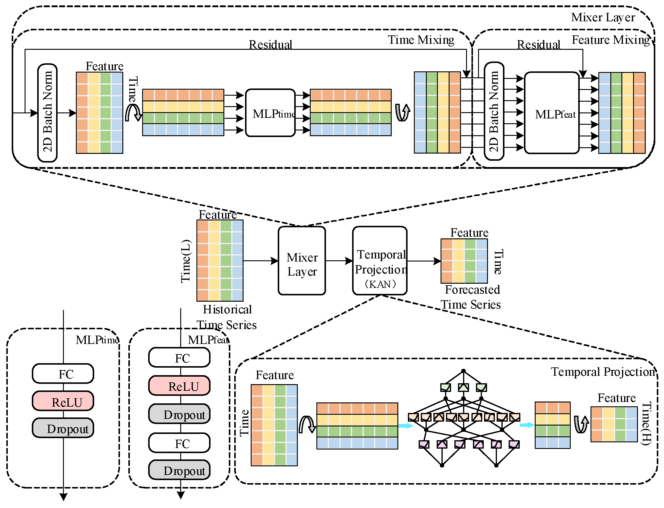
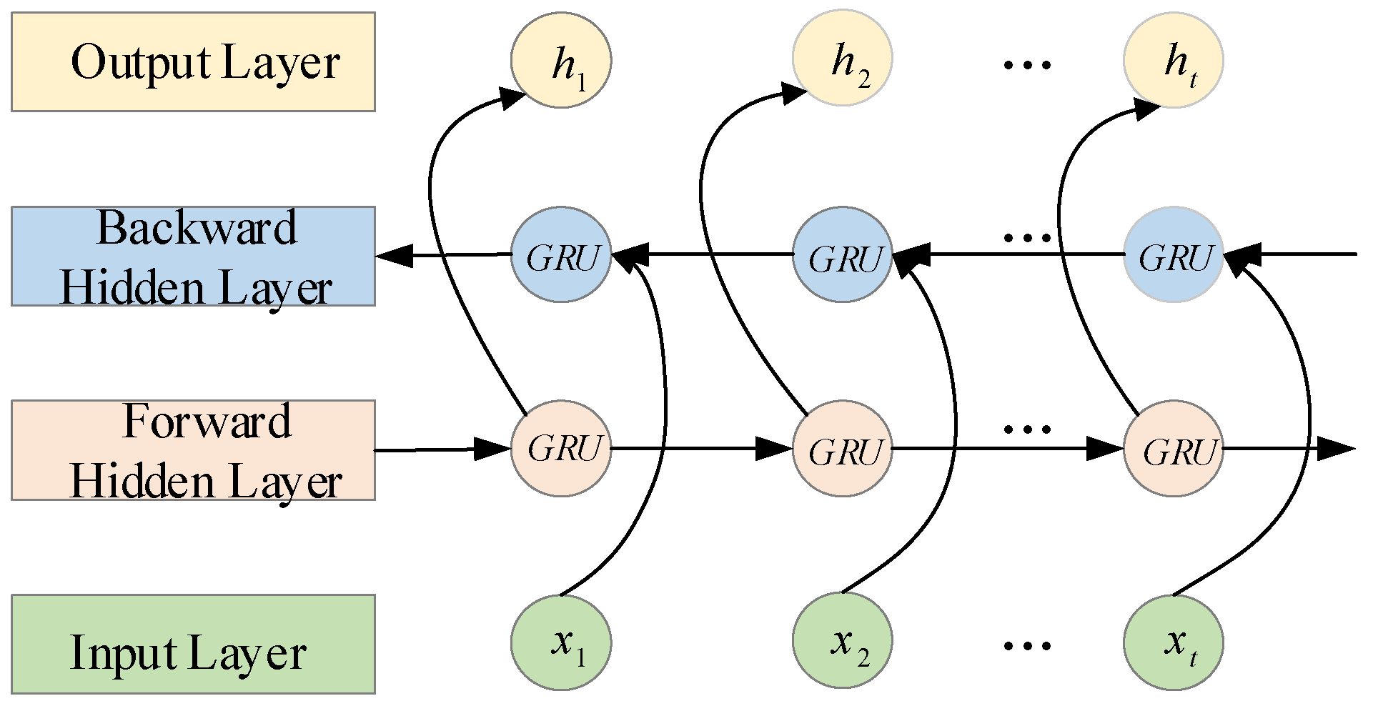
The hidden layer dimension of the TSMixer module influences its capacity to capture both temporal and feature-level representations, which in turn affects the KAN module’s ability to extract deep correlations from the feature matrix. Second, the hidden layer size of the KAN module directly impacts the model’s ability to extract high-order features. Additionally, the number of neurons in the BiGRU module must strike a balance between effectively capturing bidirectional long- and short-term dependencies and maintaining computational efficiency, thereby ensuring high prediction accuracy without overfitting or excessive resource consumption. Based on these considerations, multiple sets of comparative experiments were designed to test combinations of hidden layer dimensions in the TSMixer and KAN modules, as well as different neuron counts in the BiGRU module. The optimal configuration for each module was determined based on experimental results. With a learning rate of 0.001, a batch size of 16, and 200 training epochs, the evaluation metrics and prediction errors for the one-step carbon market price prediction experiment on the EUA dataset are presented in
Table 4 and
Figure 12.
As shown in
Table 4 and
Figure 12, the proposed TKMixer-BiGRU-SA model achieves the lowest error evaluation metrics and the prediction errors are closest to zero when the hidden layer dimensions of the TSMixer and KAN modules are set to 16 and 32, respectively, and the number of neurons in the BiGRU module is set to 32. These results indicate that the model delivers the best prediction performance under this configuration, demonstrating the strongest overall feature extraction capability and the most appropriate parameter settings.
- (2)
Model training hyperparameter configuration
Hyperparameters have a significant impact on the training performance and effectiveness of the model. Different combinations of hyperparameters can lead to notable differences in accuracy, convergence speed, and overall model behavior. By conducting comparative experiments, we can systematically and comprehensively evaluate the influence of various hyperparameter settings, visually compare the advantages and disadvantages of each combination, and accurately identify the configuration that yields optimal model performance on a specific task and dataset. The experimental results under the optimal model parameters with different training hyperparameter settings are shown in
Table 5, and the training loss curves are illustrated in
Figure 13.
The experimental results indicate that appropriately increasing the number of training epochs (epoch = 200) significantly improves performance. The combination of batch size = 16 and learning rate = 0.001 achieves the best trade-off between error and model fitting, yielding the lowest eRMSE (0.0648) and the highest R2 (0.9997), while maintaining good training efficiency (323 s). In contrast, an excessively large batch size or an overly small learning rate leads to performance degradation. Overall, the 200-16-0.001 configuration proves to be the optimal and most stable setting, demonstrating a favorable balance between training efficiency and prediction accuracy.
4.2. Comparison Experiment with Different Inputs
To verify the effectiveness of the selected feature variables and the combined input strategy based on decomposition methods, a series of experiments were designed as follows:
B1: uses the original carbon price data as a single-branch model input.
B2: builds upon B1 by adding relevant feature variables filtered through Pearson correlation analysis, still using a single-branch input.
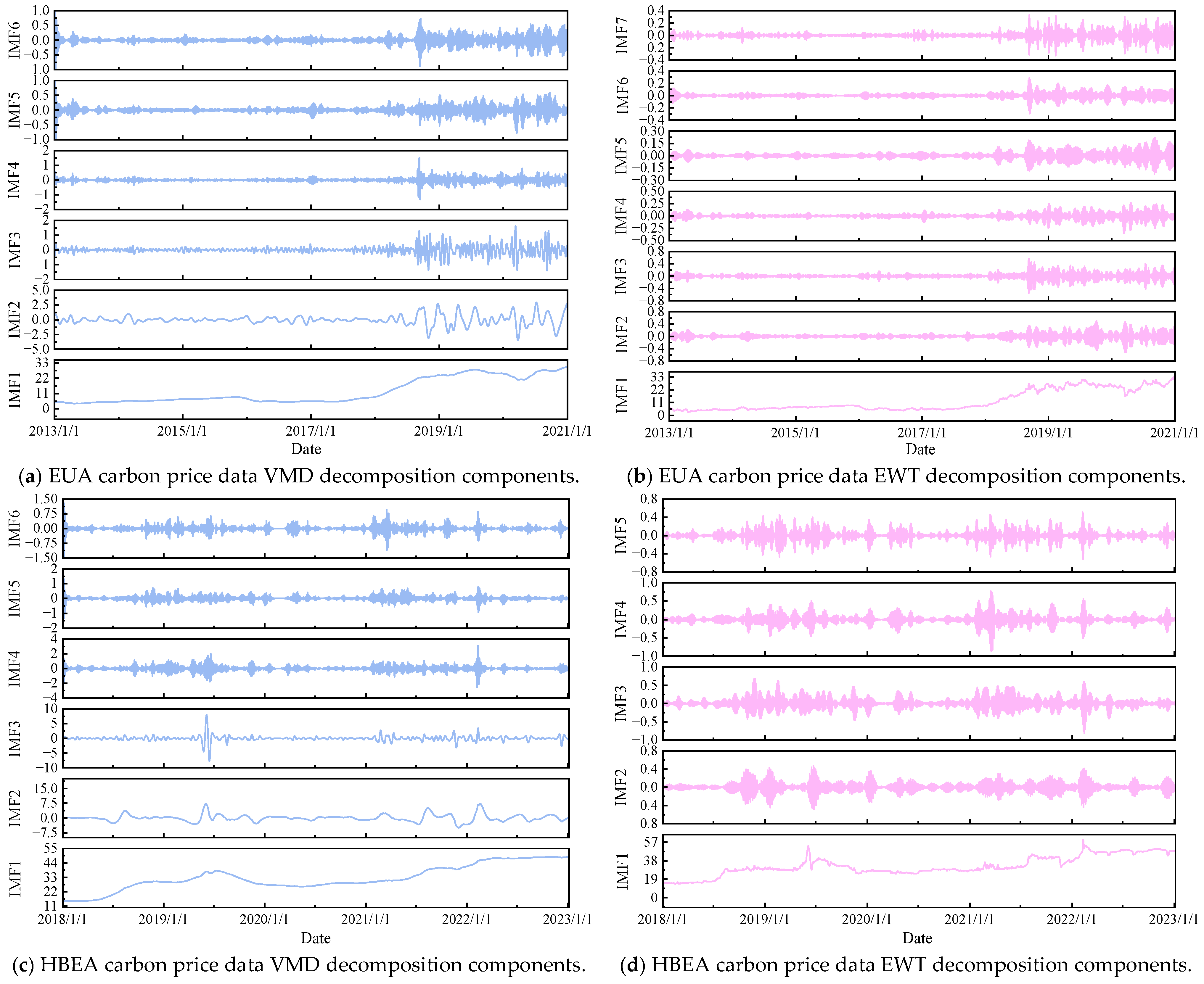
B3: extends B2 by incorporating the VMD-decomposed components of the original carbon price series, forming a dual-branch model input.
B4: builds upon B2 by introducing EWT-decomposed components of the original carbon price series, maintaining a dual-branch structure.
B5: builds upon B2 by introducing CEEMDAN-decomposed components of the original carbon price series, maintaining a dual-branch structure
B0: combines the inputs from B2, B3, and B4 to form a full three-branch model input.
Traditional model frameworks have primarily focused on single-step prediction, where deep learning models infer the next day’s carbon price based solely on historical closing prices. However, multi-step prediction offers a significant advantage by uncovering longer-term trends in price dynamics, providing broader and more strategic insights for market decision-making.
To assess the model’s performance in multi-step forecasting scenarios, this study employs carbon price data from the EUA and HBEA markets and conducts forward prediction experiments for two-step, three-step, and four-step horizons. Specifically, two-step forecasting aims to estimate the carbon prices for the two trading days following the end of the training set; three-step and four-step forecasts extend this prediction window accordingly.
All experiments were conducted using the proposed TKMixer-BiGRU-SA model and its core variants. The prediction errors on the test sets for both datasets are presented in
Table 6, and the linear regression results between predicted and actual values are shown in
Figure 14.
The analysis results indicate that under the forecasting scenarios 1–4 steps ahead, prediction accuracy generally declines as the forecasting horizon increases. However, compared to other input configurations, the proposed input strategy in experiment B0 consistently yields the lowest error levels across all forecast lengths. Furthermore, analysis of the normal distribution of prediction errors across different prediction step sizes shows that B0 achieves the smallest mean and standard deviation of errors, indicating higher model stability and reliability. These findings provide strong evidence supporting the predictive capability of the proposed model.
For the EUA dataset, Experiment B0 outperforms all other configurations across the four evaluation metrics. Specifically, in the one-step forecast, the model achieves an eRMSE of 0.0648, an eMAE of 0.0504, an eMAPE of 0.2081%, and an R2 of 0.9997, demonstrating high prediction accuracy and an excellent fit. In the four-step forecast, comparative experiments B1 through B5 demonstrate the effectiveness of various input configurations. Compared with B1, B2 achieves a 1.127% reduction in eMAPE and a 0.6459% improvement in R2, indicating that the inclusion of relevant variables enhances the model’s sensitivity and accuracy by providing a more comprehensive representation of carbon price dynamics. Further, B3 and B4 show significant improvements over B2, with eMAPE reductions of 51.732% and 12.8966%, and R2 increases of 6.3309% and 1.7840%, respectively. These results indicate that the introduction of VMD and EWT decomposition branches substantially enhances prediction performance. The VMD algorithm effectively decomposes nonlinear and non-stationary signals, while the EWT algorithm extracts amplitude- and frequency-modulated components, both of which help uncover the intrinsic patterns of carbon price fluctuations. Although B5 shows relatively high performance metrics compared to B3 and B4, its slightly inferior accuracy suggests that CEEMDAN, despite decomposing the original signal into a greater number of components, may introduce additional noise-like disturbances, leading to overfitting and reduced prediction precision. Compared with B3 and B4, B0 achieves eMAPE reductions of 33.3514% and 63.0667%, and R2 increases of 1.4629% and 5.9955%, respectively. These results underscore that integrating additional input data leads to a more comprehensive and accurate predictive model.
For the HBEA dataset, similar trends are observed, further validating the superiority of the three-branch input structure. In the one-step prediction experiment, configuration B0 achieved the best performance across all four metrics—eRMSE, eMAE, eMAPE, and R2—registering values of 0.0884, 0.0664, 0.1389%, and 0.9968, respectively. The worst performance was observed in B1 and B2, differing from the results on the EUA dataset. This discrepancy may stem from the developmental stage of the Hubei carbon market, which is likely less mature and characterized by relatively simpler and more stable price dynamics. Furthermore, Hubei’s market data may be influenced by factors such as policies, quota allocations, and enterprise behavior. In this context, VMD and EWT decomposition techniques can effectively extract more critical features from the raw data, thereby improving prediction accuracy.
In summary, the proposed dual-modal decomposition tri-branch input model achieves higher forecasting accuracy and lower prediction error, effectively demonstrating the validity of the improved input strategy and providing a strong foundation for future forecasting research.
4.3. Ablation Experiment
To evaluate and understand the importance of each module within the deep learning model and its impact on overall performance, this study conducts ablation experiments. By observing how modifications to the model structure affect its performance and outputs, the goal is to identify the most optimized architecture, improve efficiency, and enhance the interpretability of the proposed TKMixer-BiGRU-SA model. The experimental configuration is as follows:
C1: TSMixer.
C2: TKMixer.
C3: BiGRU.
C4: TKMixer-BiGRU.
C0: TKMixer-BiGRU-SA (proposed model).
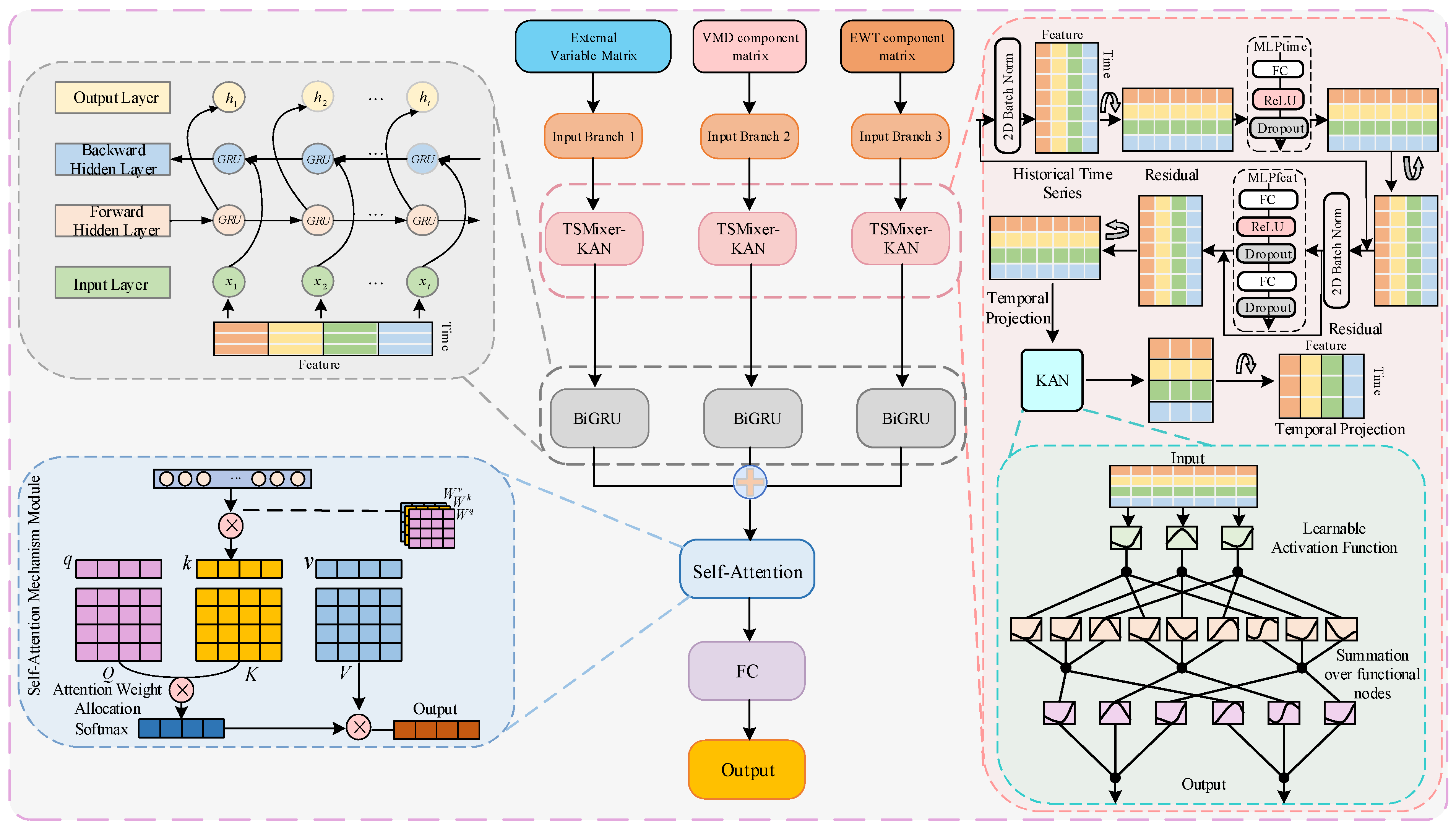
Configuration C1 and C3 represent baseline models using only the TSMixer or BiGRU modules, respectively, within the three-branch deep learning architecture. C2 embeds the KAN network into the temporal mapping layer of the TSMixer module. C4 combines the modules from C2 and C3 in a deep sequential structure within the same branch. C0, the complete model proposed in this study, extends C4 by integrating a Self-Attention (SA) module to validate the significance of attention mechanisms in optimizing model performance and improving prediction accuracy.
Table 7 presents the performance metrics of the model architectures under different ablation experiment configurations. As shown, the models in experiments C1 and C3, which adopt a single basic module, exhibit relatively low parameter counts and floating-point operations, resulting in faster training. This efficiency is primarily attributed to the simplicity of the module structures. However, these configurations demonstrate limited feature extraction capability, leading to lower prediction accuracy. In contrast, experiments C2 and C4 incorporate both the KAN and BiGRU modules, which significantly enhance the model’s ability to capture complex data features. This improvement, however, comes at the cost of increased model parameters and computational complexity, thus reducing training efficiency. Experiment C0 represents the full model proposed in this study, which integrates the strengths of multiple structural modules. Although this configuration leads to increased model complexity and longer training time, it achieves superior prediction accuracy compared to the other configurations. The increase in computational overhead remains within an acceptable range. Therefore, the moderate trade-off between accuracy and efficiency—achieved through a multi-module collaborative architecture—proves to be a rational and effective design choice.
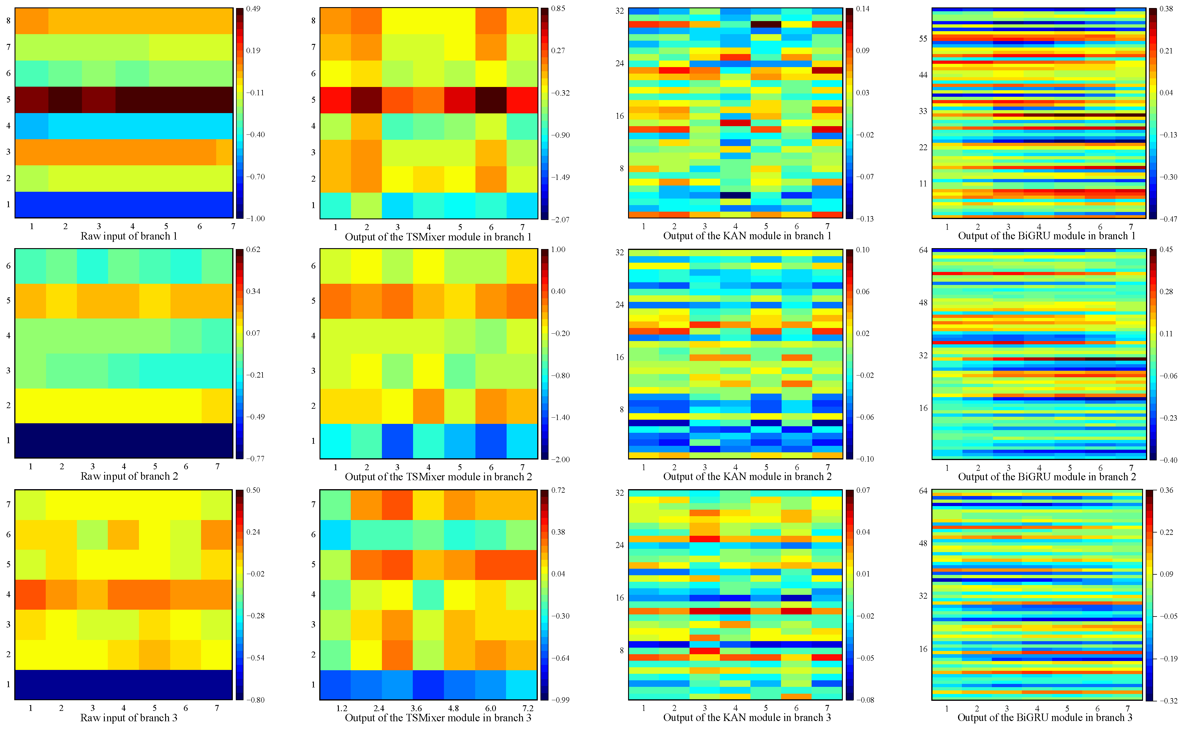
Taking the one-step prediction experiment on the EUA dataset as an example, the features extracted by each module from a single input are visualized using pseudo-color images, as shown in
Figure 15. A comparative analysis of the visualized features from the three-branch structure reveals significant differences between the feature maps extracted from the carbon price subcomponent matrix—generated via the hybrid VMD + EWT decomposition—and those extracted from the external factor matrix. This demonstrates the effectiveness of the proposed scheme in capturing multi-scale features inherent in the carbon price data. Under optimal parameter settings, the features extracted by the different modules exhibit considerable variation, indicating that the sequential arrangement of submodules contributes to feature complementarity. This, in turn, provides valuable references for the Self-Attention (SA) module to effectively focus on key temporal features.
All five configurations are trained using the tri-branch input framework. The prediction curves for the test sets of the EUA and HBEA datasets are shown in
Figure 16 and
Figure 17, respectively, and the corresponding prediction error metrics are summarized in
Table 8.
EUA dataset: A comparative analysis between experiments C1 and C2 reveals that integrating the KAN module into the baseline TSMixer architecture significantly improves model performance. Compared to the original TSMixer model, the TKMixer configuration achieves substantial reductions in all error metrics. Specifically, R2 values increase to 0.9986, 0.9962, 0.9915, and 0.9906 across the 1–4 step prediction horizons, validating the effectiveness of the KAN module in extracting high-order features and enhancing feature representation.
Further comparisons between C4 and both C2 and C3 show that, in one-step forecasting, C4 reduces eRMSE by 34.7440% and 42.2007%, eMAE by 11.3200% and 47.6673%, and eMAPE by 31.4208% and 46.3130%, respectively. These results demonstrate that the TKMixer structure enables efficient feature mixing and transformation, strengthening temporal dependencies and expressiveness. When coupled with BiGRU’s bidirectional dependency modeling, the combined architecture accurately captures critical features in the input sequence, leading to significantly improved prediction performance.
C0, the full model incorporating the Self-Attention (SA) mechanism, further enhances prediction accuracy through dynamic weighting of feature importance. Under this configuration, eMAPE drops to 0.2081%, 0.5660%, 0.8293%, and 1.1063% for 1–4 step predictions, while R2 reaches 0.999, 0.9978, 0.9957, and 0.9918, respectively.
As shown in
Figure 11, the predicted values from the proposed model closely align with the ground truth, with minimal fluctuations and positioning near the center of the 95% confidence interval for all comparative predictions. The predicted mean curve closely follows that of the true values, while
eRMSE,
eMAE, and
eMAPE all exhibit a clear inward contraction, and R
2 shows a pronounced outward expansion. These consistent trends confirm that the proposed model achieves the lowest prediction errors and the highest fit quality, demonstrating superior forecasting performance.
HBEA dataset: The experimental results on the HBEA dataset confirm the performance trends observed in the EUA dataset, further highlighting the robustness and superior predictive capabilities of the proposed model. As shown in
Figure 17, during periods of sharp carbon price fluctuations, the proposed model closely fits the actual values. Compared to the TKMixer and BiGRU models, in the one-step forecast, the proposed model reduces
eRMSE by 41.9567% and 39.9864%,
eMAE by 51.7090% and 49.2355%, and
eMAPE by 51.5352% and 48.8586%, while improving
R2 by 0.6259% and 0.5650%, respectively.
In contrast to the EUA dataset, the HBEA dataset exhibits more pronounced volatility and uneven historical data distribution, which increases the difficulty of prediction. The TKMixer model tends to underestimate in low-price regions, resulting in larger errors, while the TKMixer-BiGRU model overestimates in high-price regions, also leading to increased errors. In comparison, the proposed model produces predictions that closely follow the actual curve, especially around the average value of the test set, with reduced fluctuations in the fitting line. Moreover, the inward contraction of error metrics such as eRMSE, eMAE, and eMAPE, alongside the outward increase in R2, reinforces that the proposed model yields the lowest prediction errors and the highest degree of fit. However, R2 values for the HBEA test set under 1–4 step forecasts—0.9968, 0.9926, 0.9755, and 0.9726—are slightly lower than those from the EUA dataset. This difference is attributed to the higher complexity and volatility of the HBEA data, as well as external influences such as China’s carbon reduction policies (e.g., mitigation actions, nationally determined contributions, and carbon neutrality goals), which were not explicitly modeled.
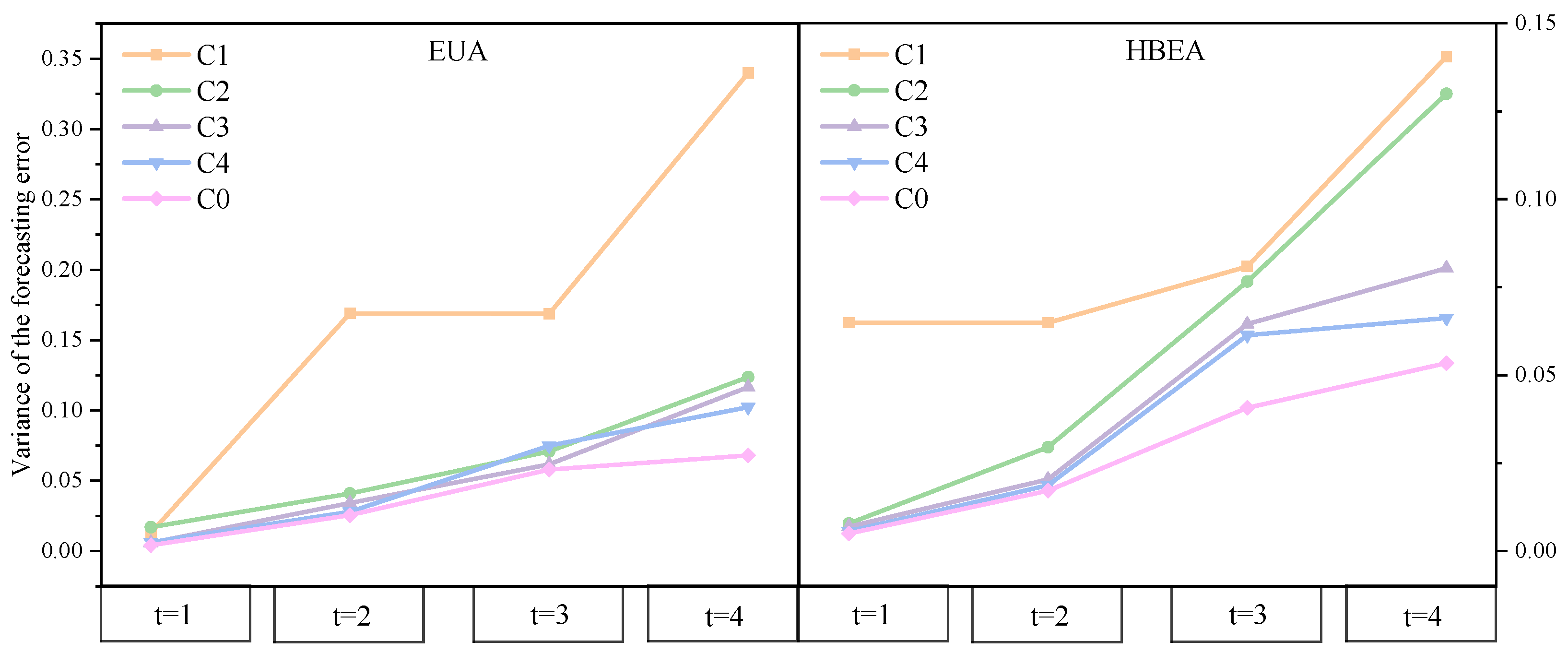
Figure 18 and
Table 9 present the variance of prediction errors and the results of paired-sample
t-tests across different model configurations on the EUA and HBEA datasets. Variance-based comparative analysis demonstrates that the proposed TKMixer-BiGRU-SA model consistently outperforms others on both datasets, achieving the lowest and most stable error variances across one- to four-step forecasts, thus exhibiting a clear competitive advantage.
The paired-sample t-test results further confirm that integrating the KAN module into the TSMixer architecture (C1 vs. C2) leads to significant improvements in multi-step prediction performance, particularly enhancing stability on the HBEA dataset. This highlights the KAN’s effectiveness in capturing complex temporal dependencies. Moreover, introducing the BiGRU structure (C2 vs. C4) yields notable performance gains at all prediction horizons, validating the importance of bidirectional contextual modeling in sequence prediction.
The combination of TKMixer with BiGRU (C3 vs. C4) also consistently achieves statistically significant improvements, underscoring the synergistic effect between these components as a key driver of model performance enhancement. Building upon C4, the incorporation of the Self-Attention mechanism (C4 vs. C0)—as in the proposed final model—delivers additional performance gains at most time steps, with particularly pronounced improvements at t = 1 and t = 2. This demonstrates the model’s enhanced capacity to focus on critical temporal features. However, minor performance fluctuations observed at a few time steps suggest that the application of attention mechanisms should be carefully tailored to task-specific characteristics.
Overall, these experimental findings validate the effectiveness and robustness of modular composition in improving prediction performance and highlight subtle yet statistically significant differences between competing model architectures.
4.4. Comparison Experiment with Different Literature
To validate the superiority of the proposed forecasting scheme compared to various existing models and methods reported in current research, this study conducted a series of comparative experiments.
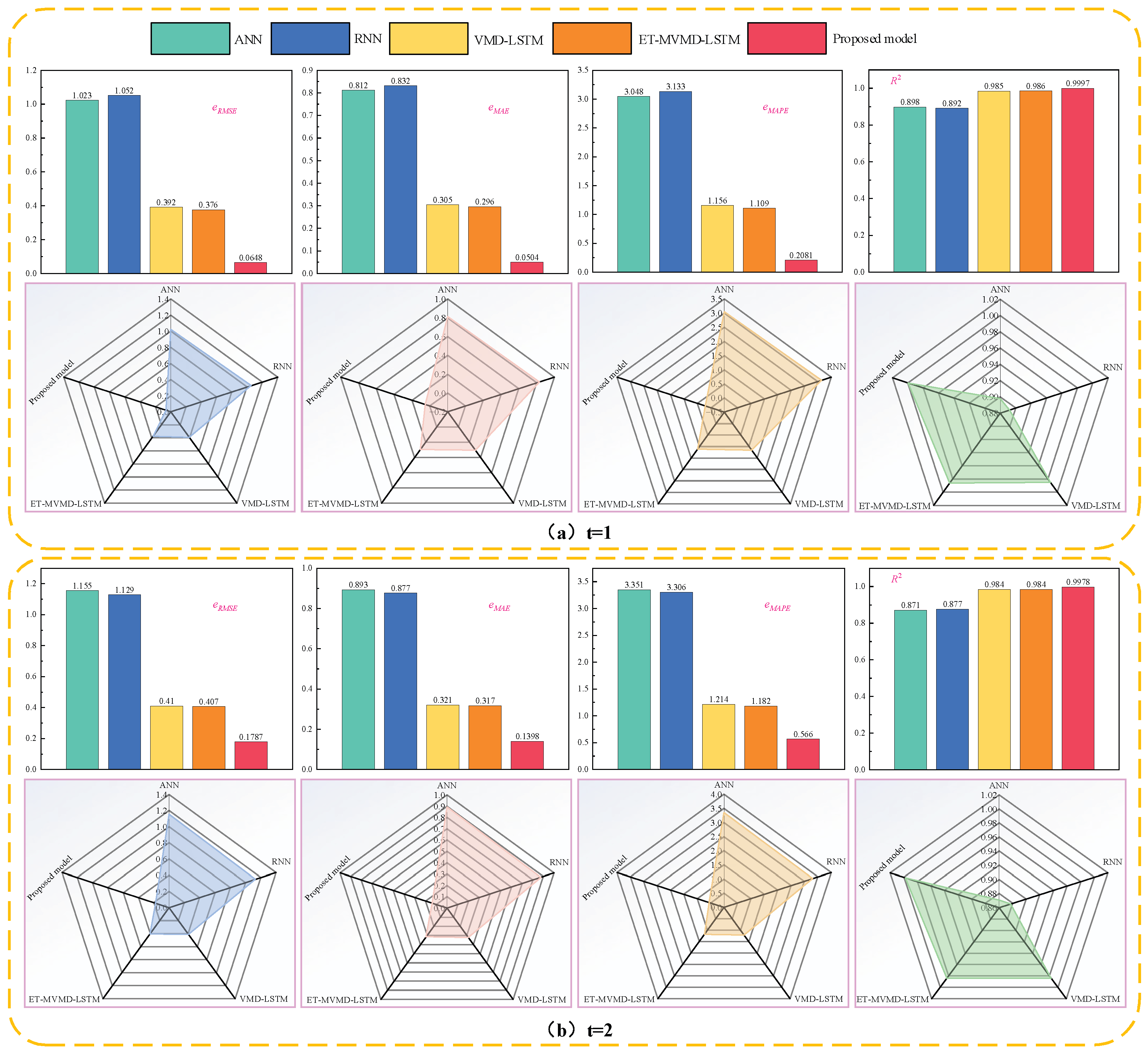
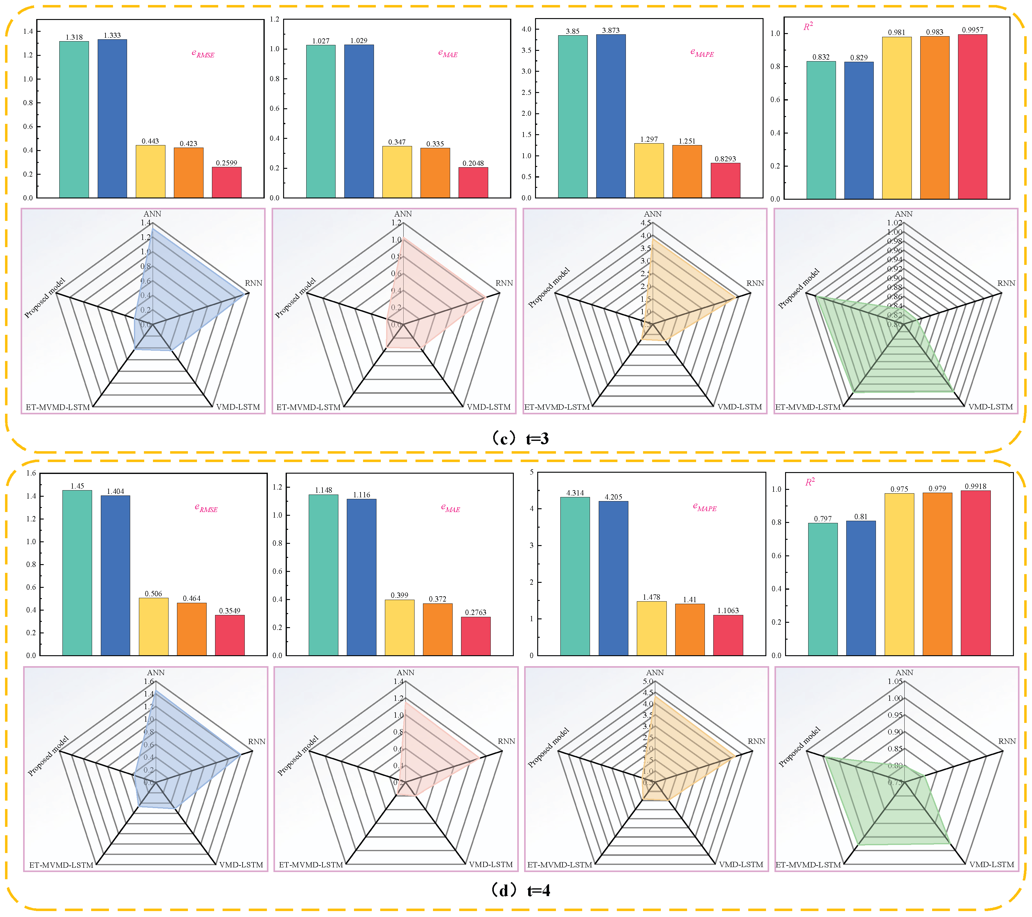
Using the EUA carbon price data from 1 January 2013 to 1 January 2021 as an example, the prediction error metrics of the method presented in [
36] and those of the proposed model are compared. As shown in
Figure 19, the proposed method demonstrates clear advantages in terms of prediction accuracy across all evaluated metrics.
As shown in
Figure 19, the prediction difficulty increases with the forecasting horizon. This is reflected in the rising values of
eRMSE,
eMAE, and
eMAPE, along with a decreasing
R2, indicating a decline in predictive accuracy. The ET-MVMD-LSTM hybrid forecasting model proposed in [
36] integrates ET-based feature selection, MVMD decomposition, and LSTM deep learning architecture. This approach effectively reduces the complexity of time series data while capturing the inter-variable correlations, enabling it to accurately model the dynamic behavior of carbon prices. It performs well even in multi-step forecasting tasks, demonstrating more stable and reliable performance than single models such as ANN and RNN. Specifically, for one-step forecasting, it achieves an
eRMSE of 0.376,
eMAE of 0.296,
eMAPE of 1.109%, and an
R2 of 0.996.
In contrast, the TKMixer-BiGRU-SA model proposed in this study maintains high prediction fidelity across 1 to 4-step ahead forecasts. Notably, for the four-step forecast, the model achieves an
eMAPE of just 0.2081% and an
R2 of 0.9997. Compared to the ET-MVMD-LSTM model from [
36], the
eMAPE of our model is reduced by 81.2353%, 52.1151%, 33.7090%, and 21.5390% for 1–4 step predictions, respectively. These results strongly support the effectiveness and robustness of our model in handling complex and challenging prediction tasks.
Regarding the HBEA dataset,
Figure 20 presents a comparison of one-step forecasting error metrics between our proposed model and those from [
37,
38,
39]. The TKMixer-BiGRU-SA model consistently achieves the lowest
eRMSE,
eMAE, and
eMAPE, and the highest
R2 among all methods. Specifically, compared to the traditional ARIMA model from [
37], the proposed model reduces
eRMSE,
eMAE, and
eMAPE by 82.4777%, 82.3591%, and 88.9057%, respectively—highlighting the limited predictive power of single models in capturing complex data features.
By integrating suitable decomposition strategies and leveraging complementary strengths of hybrid deep learning models, our approach effectively utilizes multidimensional features of carbon price data and its external factors, leading to a significant improvement in predictive performance. Compared with the VMD-AWLSSVR-PSOLS-WSM model [
37], the HI-TVFEMD-transformer model [
38], and the Informer-DABOHBTVFEMD-CL model [
39], our method achieves reductions in
eRMSE,
eMAE, and
eMAPE of 50.9433%, 79.4705%, and 58.7879%; 53.5989%, 56.9390%, and 51.3909%; and 70.3142%, 66.1220%, and 52.1034%, respectively. Additionally, the
R2 reaches as high as 0.9968. The potential overfitting in previous models may stem from overlapping functionalities and excessive parameter complexity in their hybrid architectures, despite employing signal decomposition techniques. In contrast, our model effectively balances data decomposition and feature extraction, maximizing the performance of each module and validating the soundness of our methodological design.


